
Abstract
This article examines the stochastic response of a system with a Bingham model magneto-rheological damper under random excitation. The application of the stochastic averaging method yielded the averaged stochastic Itô equation. The system’s steady-state response probability density function (PDF) is obtained by solving the corresponding Fokker–Planck–Kolmogorov equation. Theoretical calculations are confirmed through numerical simulation. Additionally, the study produced graphs depicting the steady-state probability density functions for system energy, amplitude, displacement, and velocity, along with time history graphs, joint probability density functions for displacement and velocity, and continuous wavelet coefficient energy distribution graphs. The paper also examines the impacts of viscous damping, Coulomb damping, and noise intensity on the steady-state response from both time-domain and frequency-domain perspectives. The findings indicate that in this stochastic model, when velocities are relatively low, an equivalent increase in Coulomb damping has a more pronounced effect on the steady-state response than viscous damping. These results provide a theoretical basis for understanding and addressing the behavior of Bingham model magnetorheological dampers in nonlinear systems under stochastic excitation.
Keywords
Introduction
Vibration is a common phenomenon in nature, yet its potential for harm cannot be ignored. Whether it is the discomfort felt when riding in an automobile or the destruction of bridges caused by earthquakes and windstorms, vibration is closely related to our lives. Therefore, how to effectively control the occurrence of vibration to minimize the damage it may cause has been the core issue that many scholars continue to study.
As a superior semi-active control device, magnetorheological fluid damper precisely changes the damping characteristics of magnetorheological fluid by adjusting the control current to realize effective vibration suppression.1,2 The models commonly used to describe the performance of magnetorheological fluid dampers mainly include the Bingham model, hyperbolic tangent model, Bouc–Wen model, viscous Dahl model, and algebraic model, etc.,3,4 which provide the theoretical basis for the performance study of magnetorheological dampers. Thanks to its advantages of simple structure, cost-effectiveness, rapid response, and reliability,5–9 the magnetorheological damper has become an important device in the field of engineering vibration control and has been widely used in many technological fields such as aerospace, automobile, and medical equipment. The research in recent years has made remarkable progress. Fu et al. 10 investigated the mechanical effects of temperature on magnetorheological fluid dampers by setting up a test system to measure the dampers’ damping force. They discovered that the damping force reduces as the temperature increases. Ruan et al. 11 explored a new type of magnetorheological fluid damper, systematically analyzing the influence of current, velocity, frequency, and displacement on the damping force. Jiang et al. 12 developed a heavy-duty six-degree-of-freedom semi-active vibration isolation system centered around magnetorheological fluid dampers, and through design, numerical simulation, and experimental validation, proved that the system effectively lessens the vibrations transmitted through the platform to the isolation system. Ma Shengnan et al. 13 analyzed the dynamic response of magnetorheological (MR) dampers and found that the rheological response is solely related to the gap and the dynamic viscosity. Yu et al. 14 analyzed the nonlinear and hysteresis characteristics of MR dampers under ceiling control and derived the bifurcation criteria for the system under different nonlinear and hysteresis parameters. Liu Huiqian et al. 15 designed a new type of damper with a dual-coil magnetic circuit structure and conducted tensile tests on the dampers. The tests showed that, compared to single-coil structures, the dual-coil magnetic circuit produces greater damping force and reaches a steady state more quickly under the same conditions. Kim et al. 16 established a mathematical model of MR dampers using the describing function method and studied the impact of parameters on the dynamic behavior of the MR damper rotor. Zhang Wanjie et al. 17 used the averaging method to study a damping vibration reduction system containing a fractional-order Bingham model with semi-active control and analyzed the system’s stability based on Lyapunov’s theory. Wang Lin 18 performed dynamic analysis of nonlinear systems containing the Bingham model, derived the amplitude-frequency and phase-frequency response equations of the system, obtained the stability conditions for the steady-state solution, verified the accuracy of the solutions through comparison between numerical and analytical solutions, and examined the effects of various parameters on system resonance in detail. Zhang Wenjing 19 used the averaging method to conduct a dynamic analysis of a vehicle suspension system containing a fractional-order MR fluid model, obtained approximate analytical solutions using the averaging method, solved the system’s steady-state amplitude-frequency response equation, and obtained the system’s stability conditions. The analysis also considered the impact of vibration control parameters on the effectiveness of control.
In actual engineering applications, magnetorheological damper systems often face complex and variable external environments, and ideal models under simple harmonic or deterministic excitation conditions cannot fully reflect reality. In actual systems, random factors are inevitably present. These factors may originate from environmental noise, operational errors, or material heterogeneity, etc., and they have a significant impact on the vibrational behavior of mechanical systems and the measurement accuracy of precision instruments. The introduction of random factors not only increases the complexity of system analysis and control in engineering practice but also poses a significant challenge in theoretical research, making the derivation and analysis of theoretical models more difficult.
In light of this, it becomes particularly important to explore the dynamic behavior of nonlinear systems containing the Bingham model under random excitation. In this study, we adopted a Duffing oscillator combined with the Bingham model and successfully derived the probability density equation that describes the system’s amplitude as well as the joint probability density equation for displacement and velocity through the application of the stochastic averaging method. Through numerical simulation, we verified the reliability of the obtained computational results. Furthermore, based on these equations, we drew images depicting the system’s dynamic behavior and compared and analyzed the influence of different parameters on the system’s steady-state response, providing new theoretical insights for understanding and controlling the dynamics of nonlinear systems under random excitation.
Model
First, the Bingham model of a magnetorheological damper is introduced into the nonlinear system. The physical model is depicted in Figure 1. The Bingham model of the magnetorheological damper is derived from the Bingham fluid constitutive equation of the magnetorheological fluids, composed of a coulomb friction component and a viscous damping component in parallel,
20
thus it is also referred to as the Bingham viscoplastic model. The Bingham model is characterized by its clear physical interpretation, simple structure, minimal parameters, and ease of programming. The formula for the model is as follows Nonlinear system model with Bingham model.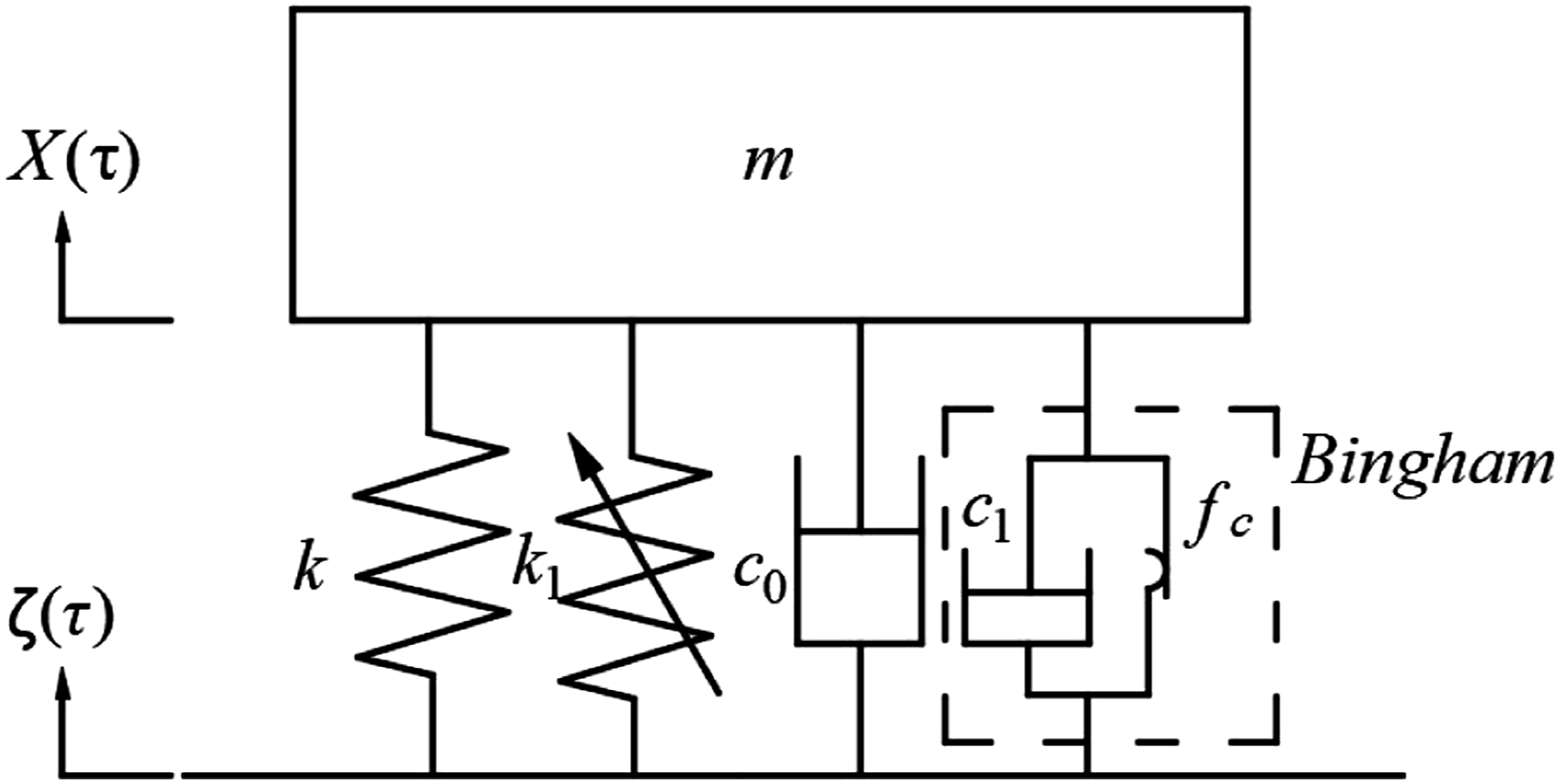


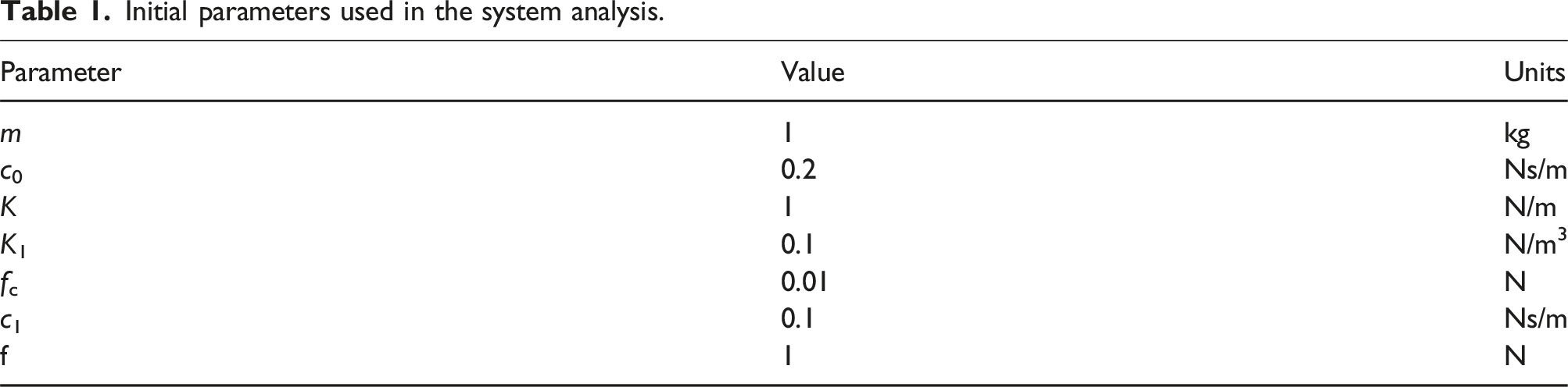
Initial parameters used in the system analysis.
Dimensionless quantization of the kinetic equation (2)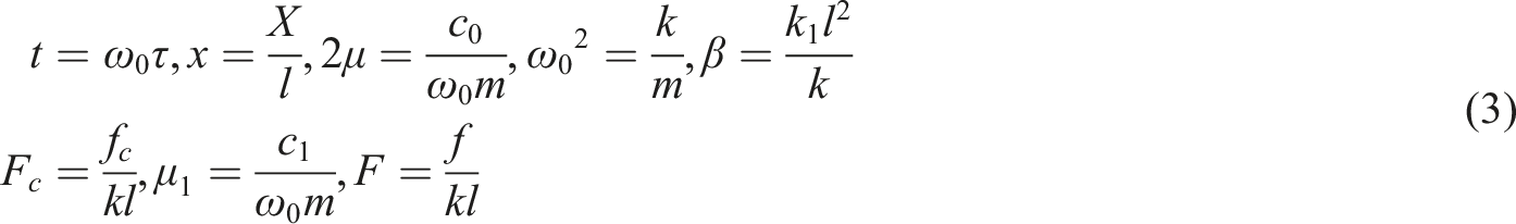

The stochastic averaging method is used to solve the dynamic equation
According to reference 21, the solution to equation (4) can be assumed to be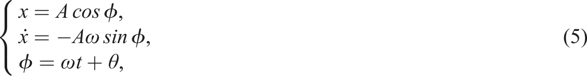
Sign function transformation (1) When (2) When (3) When 


After differentiating the first equation of (5) with respect to t and subtracting the second equation, we obtain
Differentiating the second equation of (5) with respect to t, we get
By substituting equation (11) into the dynamic equation (4) and combining it with (10), the standard equations for amplitude and phase are obtained as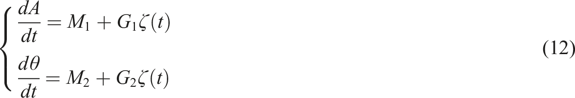
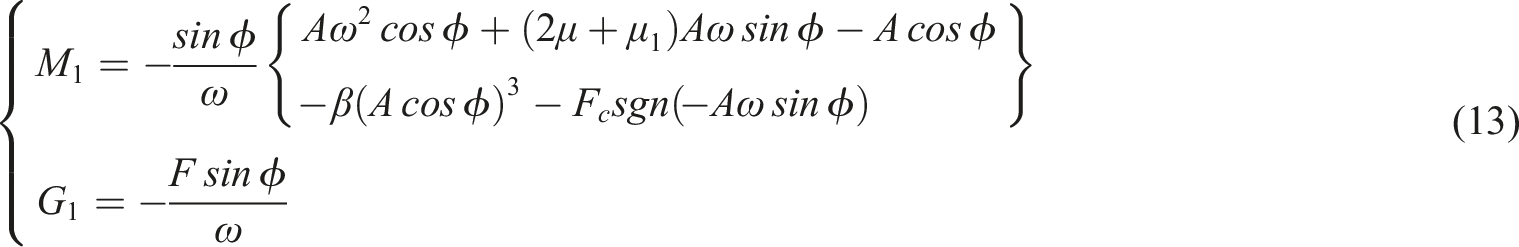
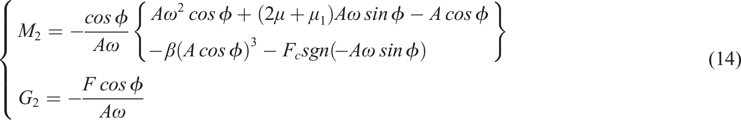
Using the stochastic averaging method22,23 and Itô's lemma, by averaging the phase over time, the deterministic stochastic average Itô differential equation for amplitude can be obtained as follows
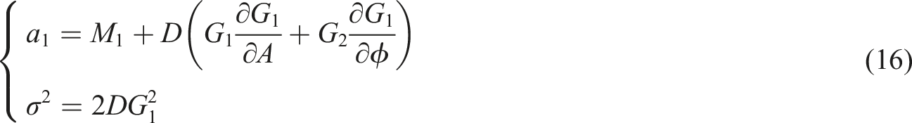
Average 

Thus
From equation (19), it can be seen that the amplitude A does not depend on the variations of 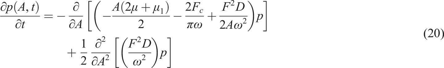
Combining equation (20) and the following boundary conditions

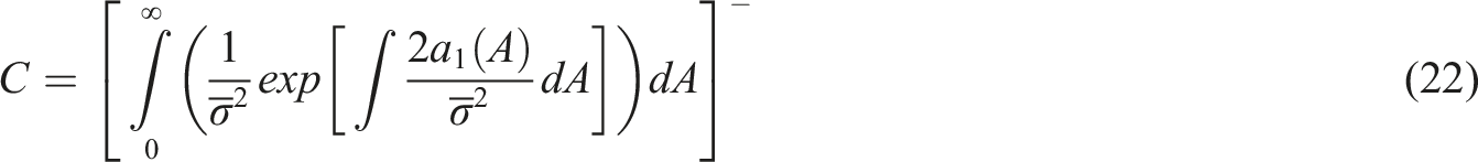
The complete expression can be obtained as follows

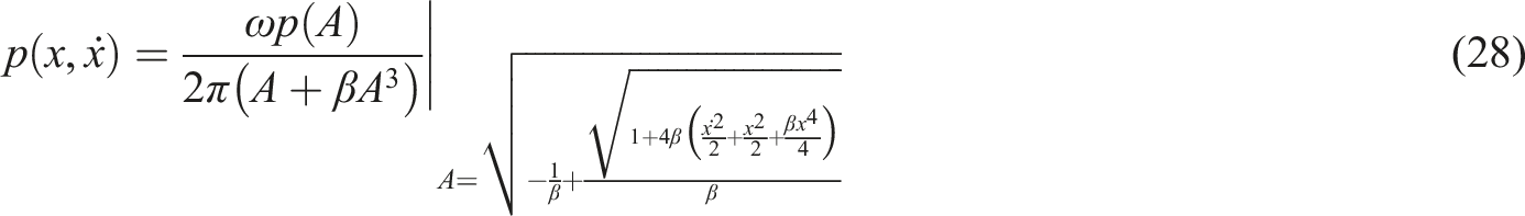
The Hamiltonian function of the system is H = U(A), and the steady-state probability density function is

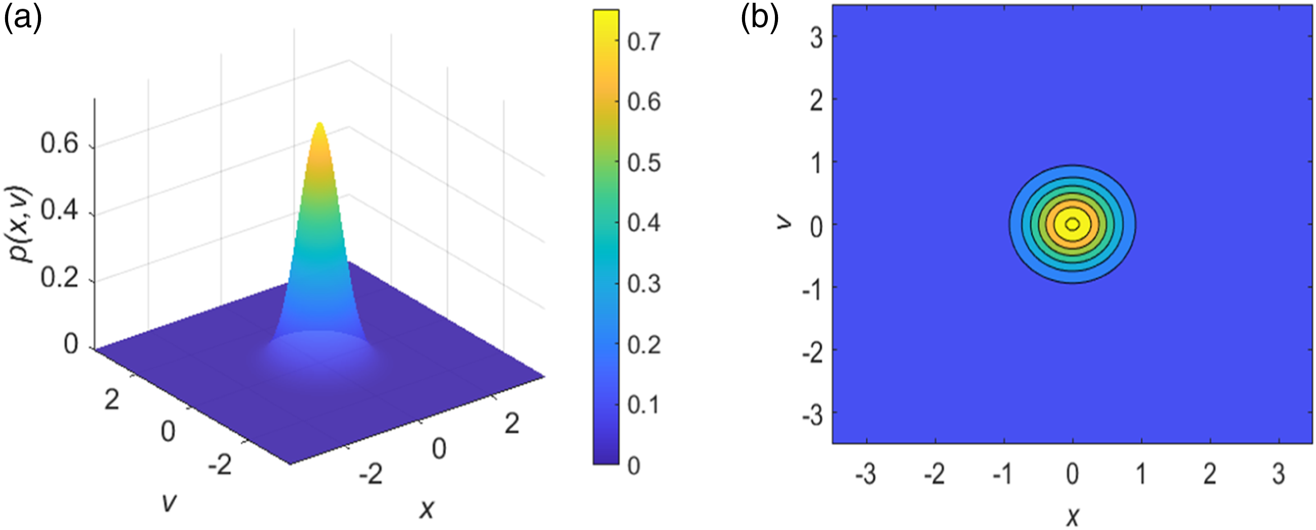
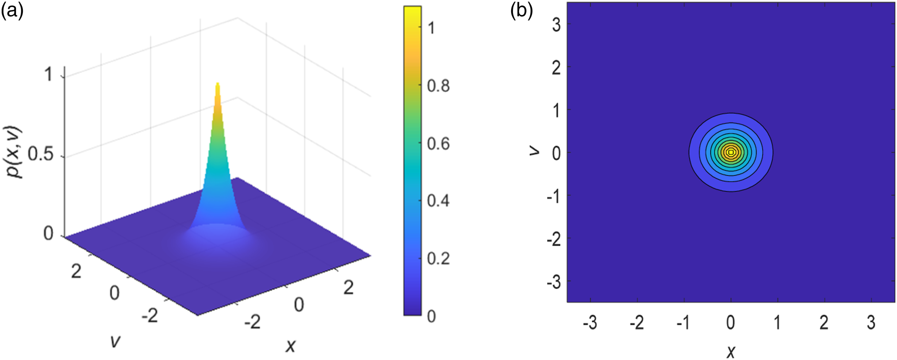
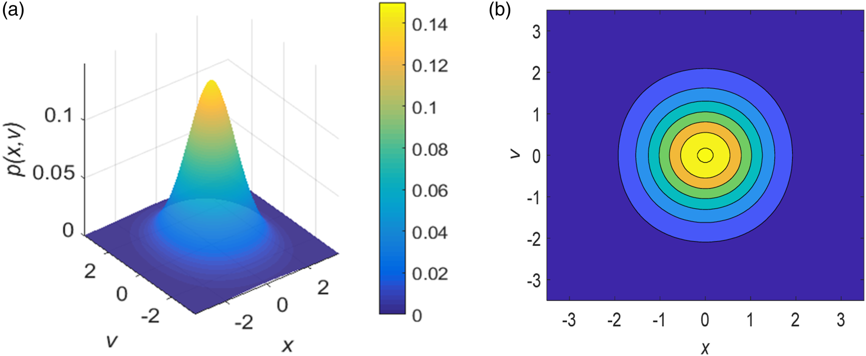
The joint steady-state probability density function for the system’s displacement and velocity is
The steady-state probability density function for displacement is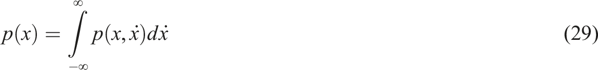
The steady-state probability density function for velocity is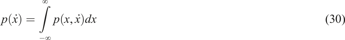
Numerical simulation
Using stochastic Runge–Kutta and Monte Carlo methods, this study set the white noise intensity at D = 0.25. We conducted simulations with 2000 noise sets, each containing 200,000 data points, directly stimulating equation (4) with a time step of Δt = 0.01. The last quarter of data points from each noise set was selected as the steady-state response and applied to the dynamical equations. Numerical solutions for the steady-state probability density functions of energy, amplitude, displacement, and velocity were plotted according to their respective relationships. Numerical simulations of the original system were performed to verify the accuracy of the analytical results. The parameters chosen for the system simulation are: Comparison chart of the System’s analytical solution and numerical solution. (a) PDF of Hamiltonian Energy H, (b) PDF of Amplitude A, (c) PDF of Displacement x, and (d) PDF of Velocity v.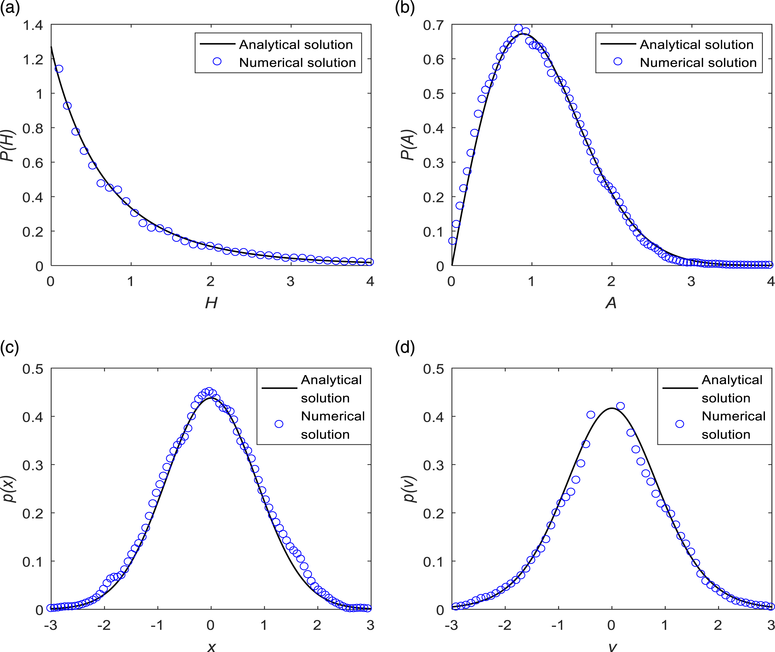
Parameter analysis
Parameter analysis is conducted through the use of Probability Density Functions (PDFs) and Continuous Wavelet Transforms to assess the impact of parameters on the steady-state response of systems. The PDF plots primarily illustrate the occurrence frequency and distribution of response amplitudes, displacements, and velocities in dynamic systems, signal processing, or other areas involving vibratory phenomena. These plots provide insights into the system’s response characteristics under random inputs, serving as a fundamental tool for understanding and optimizing system performance. In disciplines such as structural engineering, mechanical design, and signal processing, studying the PDFs offers a highly effective analytical approach.
The Continuous Wavelet Transform (CWT) is a mathematical tool used for signal analysis that transforms signals using wavelet functions. This allows for the simultaneous acquisition of time and frequency information in the time-frequency domain, enabling the determination of the frequency band range of system vibration responses. In this paper, the CWT utilizes MATLAB’s Wavelet Toolbox to process time displacements, employing the Morlet function as the mother wavelet for programming solutions.
The impact of system viscous damping on system response
Analyzing the impact of system viscous damping on system response through PDF
The following simulation parameters were selected: Graphs of three probability density functions of the system under different viscous damping coefficients. (a) PDF of Amplitude A, (b) PDF of Displacement x, (c) PDF of Velocity v. Joint probability density function of displacement and velocity at viscous damping coefficient Joint probability density function of displacement and velocity at viscous damping coefficient 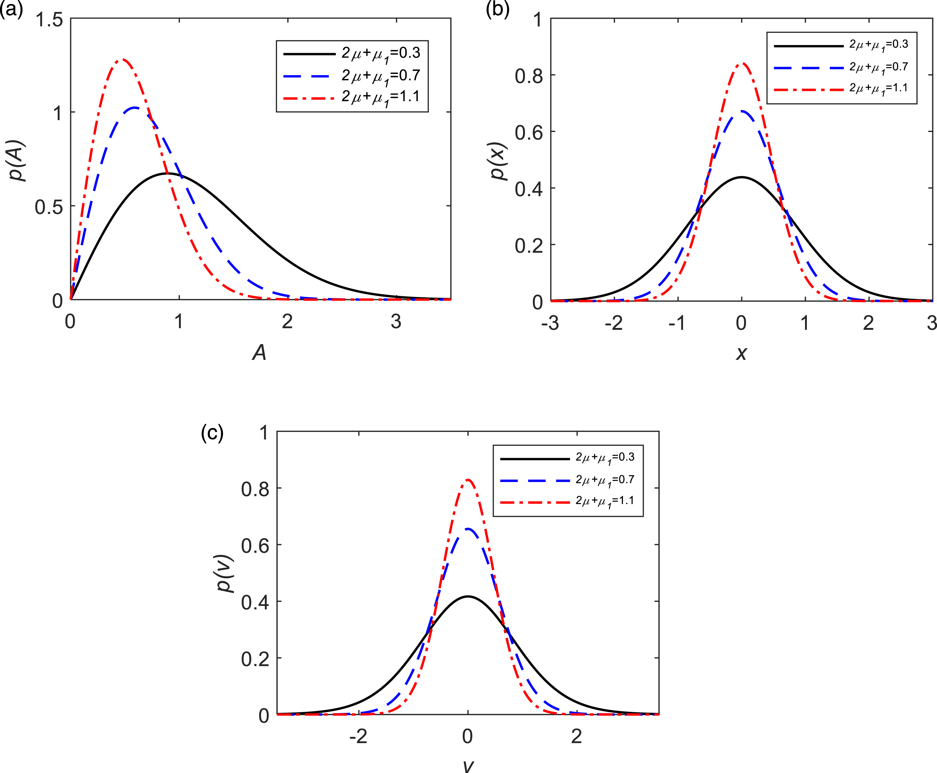
It can be observed from Figure 3 that as the viscous damping coefficient
Analyzing the impact of system viscous damping on system response via continuous wavelet transform
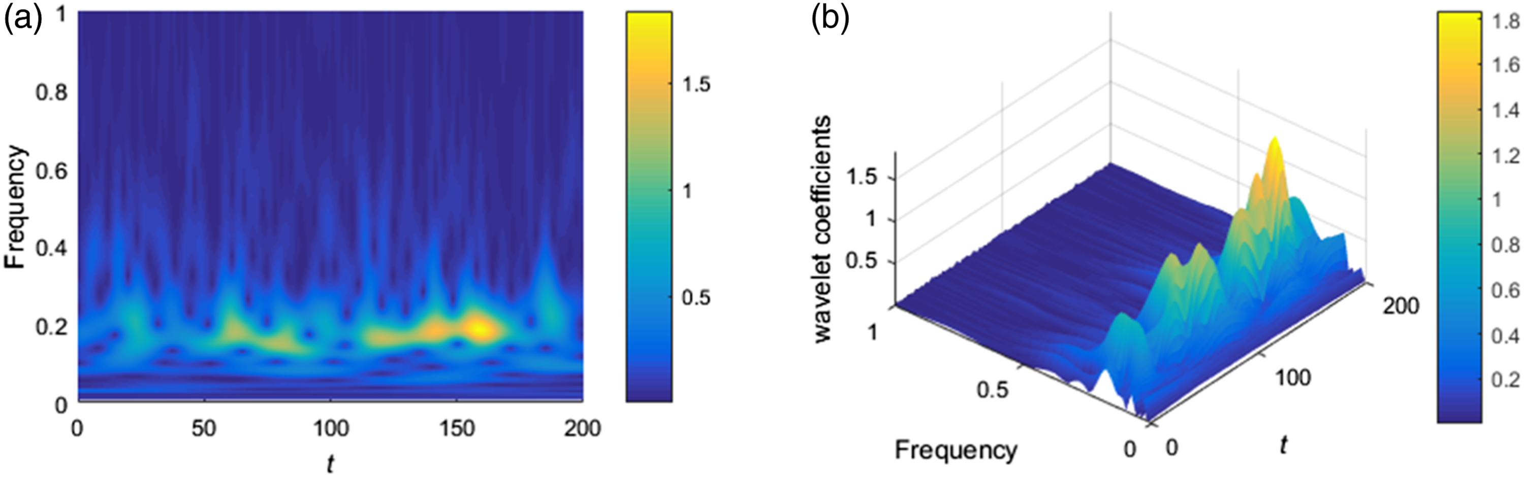
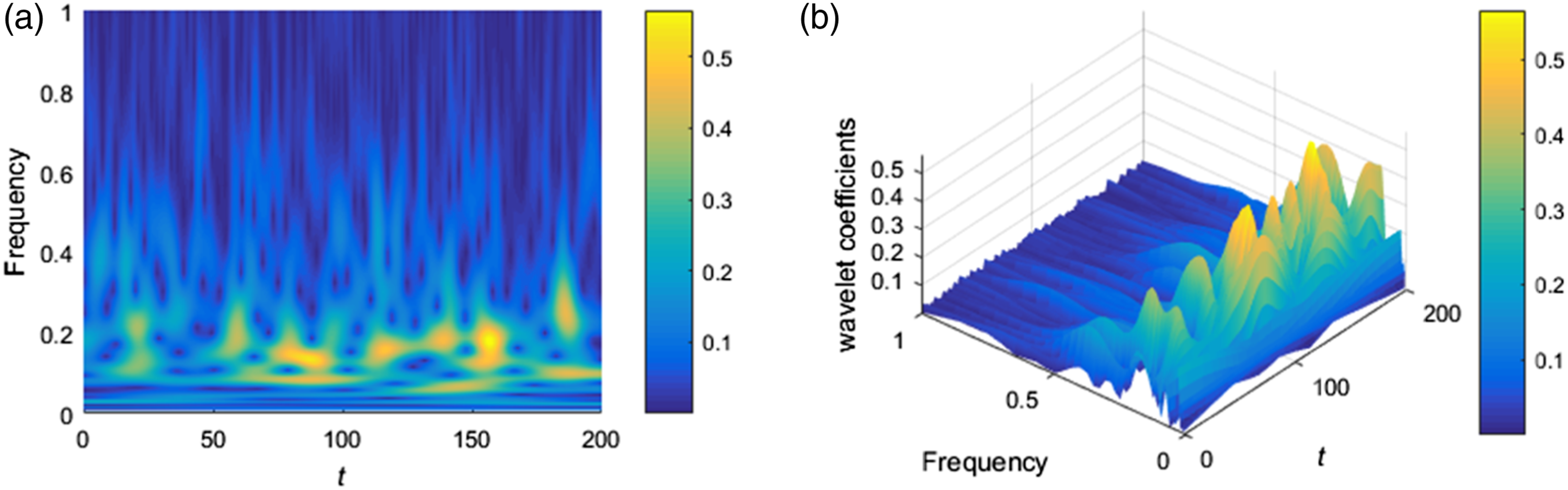
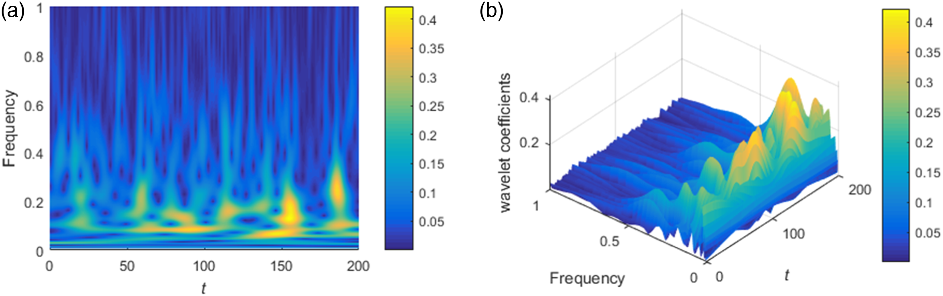
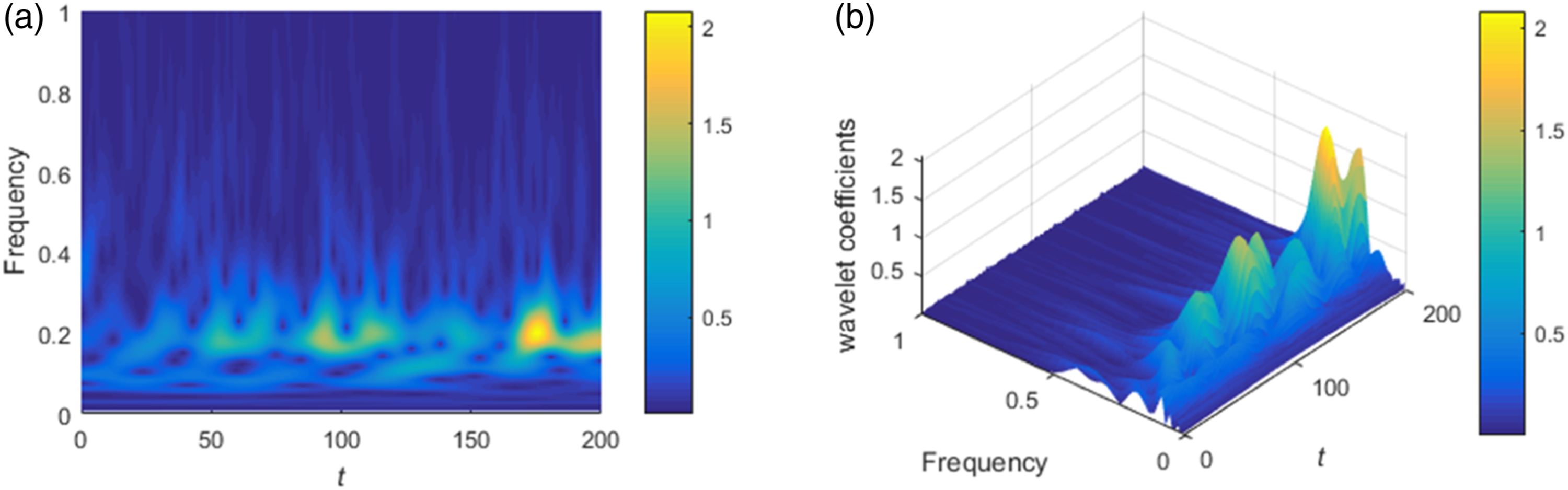
The simulation parameters are consistent with the previous ones. Figures 6 and 7 show the time histories of the system for Time-displacement and time-velocity graphs of the system at Time-displacement and time-velocity graphs of the system at Energy distribution map of continuous wavelet coefficients at Energy distribution map of continuous wavelet coefficients at 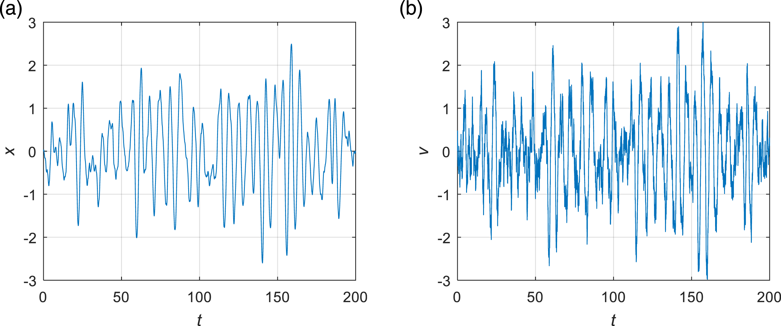
The impact of coulomb damping on system response
Analyzing the impact of coulomb damping on system response through PDF
When the Coulomb damping force Fc takes different values (0.01, 0.41, and 0.81), the steady-state probability density function graphs of the system’s amplitude, displacement, and velocity are shown in Figure 10. Figure 11 represents the joint probability density function of displacement and velocity when Fc = 0.41. It can be observed from Figure 10 that as Fc increases, the peak values of the steady-state probability density function curves for the system’s amplitude, displacement, and velocity gradually rise. At the same time, by comparing Figures 3 and 10, it can be found that this trend is similar to the behavior of viscous damping. However, a key difference is that when both the Coulomb damping force and viscous damping coefficient increase by 0.8, the changes in the three types of probability density function curves corresponding to the Coulomb damping force are more pronounced. Based on the image under the original data of Figure 4, comparing Figures 5 and 11 reveals that the increase in Coulomb damping force makes the joint probability density function graph of displacement and velocity more towering and the contour lines denser, meaning that the changes in Coulomb damping force have a more significant and sensitive impact on the system. Graphs of three probability density functions of the system under different coulomb damping forces Fc. (a) PDF of Amplitude A, (b) PDF of Displacement x, (c) PDF of Velocity v. Joint probability density function of displacement and velocity at coulomb damping force Fc = 0.41. (a) Joint Probability Density Function of Displacement and Velocity and (b) Contour Map of the Joint Probability Density Function of Displacement and Velocity.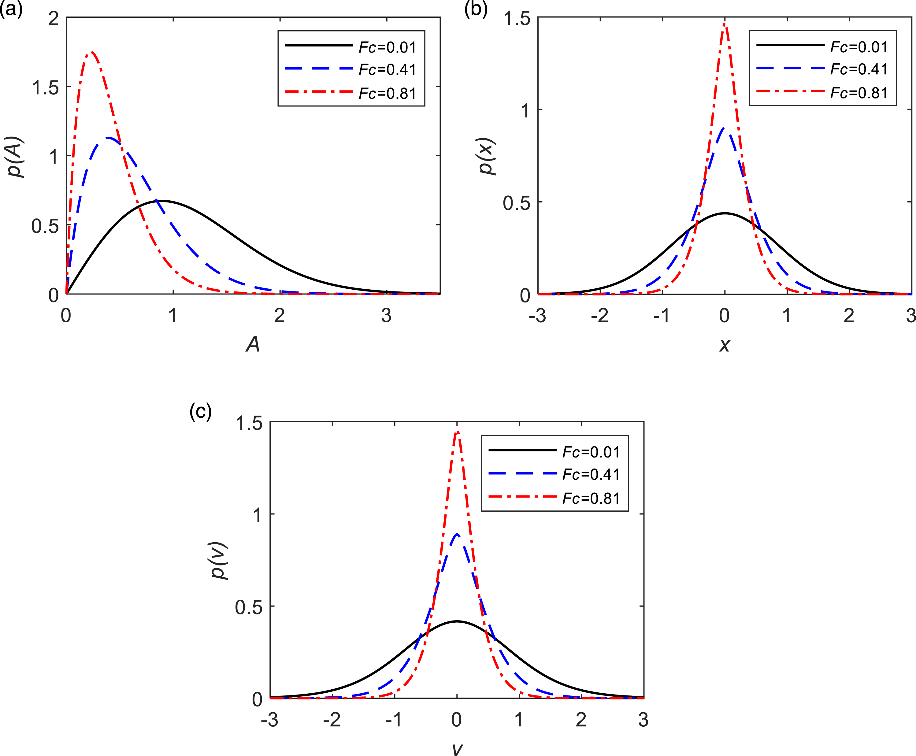
Analyzing the impact of Coulomb damping on system response via continuous wavelet transform
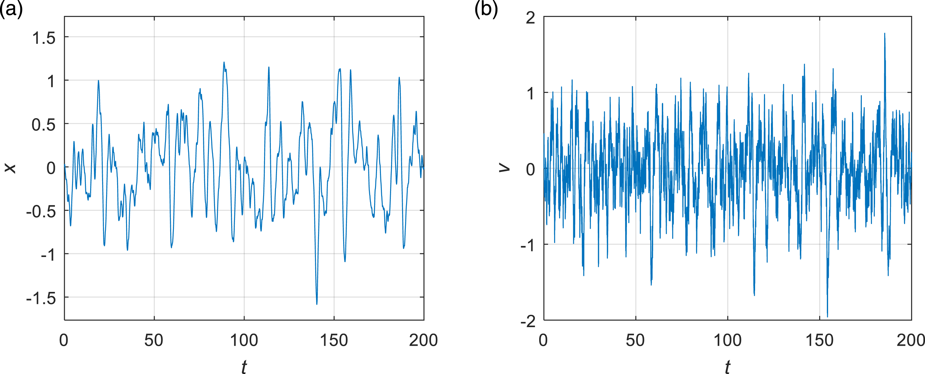
The simulation parameters remain the same. Figure 12 shows the time history of the system for Fc = 0.81. By comparing Figures 7 and 12 with the original data in Figure 6, it is observed that increasing the Coulomb damping force similarly reduces vibration displacement and velocity. However, compared to viscous damping, the changes in the time-displacement and time-velocity graphs are more pronounced for Coulomb damping in this system. This further confirms that Coulomb damping has a more significant impact on this system when the velocity is relatively low. Figure 13 presents the energy distribution of continuous wavelet coefficients for Fc = 0.81. By comparing Figures 9 and 13 with the original data in Figure 8, it can be observed that increasing the Coulomb damping force also reduces the overall energy peak and generates multiple frequency band energy peaks, producing new energy peaks in other frequency bands. The peak at 0.2 decreases significantly, gradually losing the phenomenon of energy peaks being concentrated in a single frequency band. The peak value decreases from 1.8 to 0.41, which is more pronounced compared to the peak value decrease from 1.8 to 0.52 with viscous damping. Time-displacement and time-velocity graphs of the system at Fc = 0.81. (a) Time-Displacement Graph and (b) Time-Velocity Graph. Energy distribution map of continuous wavelet coefficients at Fc = 0.81. (a) Two-dimensional map of the energy distribution of continuous wavelet coefficients and (b) Three-dimensional map of the energy distribution of continuous wavelet coefficients.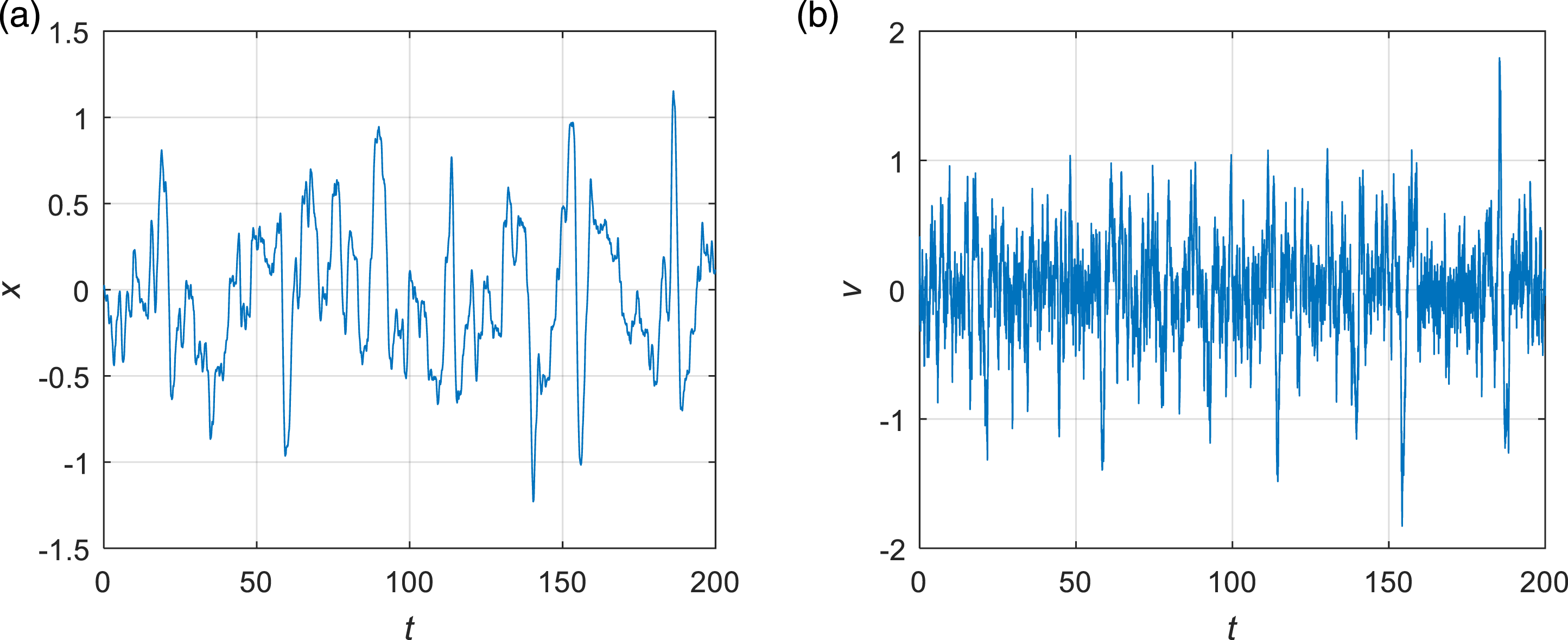
The impact of noise intensity on system response
Analyzing the impact of noise intensity on system response through PDF
When the noise intensity D is 0.25, 0.3, and 0.35, respectively, based on the impact of noise intensity on the system, it can be seen from Figure 14 that the peak values of the three curves in the figure decrease as the noise intensity increases. Combining Figures 4, 14, and 15, it is evident that the increase in noise intensity reduces the peak values of the probability density functions of system amplitude, displacement, and velocity. The greater the noise intensity, the higher the probability of the system having larger amplitude, displacement, and velocity, indicating a stronger system response. The reduction in peak values suggests that the probability of the system maintaining equilibrium decreases. The increase in noise intensity results in a lower and broader joint probability density function of displacement and velocity, indicating that the system motion becomes more intense with higher noise intensity. Therefore, in practical engineering, special attention should be paid to the impact of noise intensity on such systems. Probability density function graphs of the system under different noise intensities D. (a) PDF of Amplitude A, (b) PDF of Displacement x and (c) PDF of Velocity v. Joint probability density function of displacement and velocity at noise intensity D = 0.35. (a) Joint Probability Density Function of Displacement and Velocity and (b) Contour Map of the Joint Probability Density Function of Displacement and Velocity.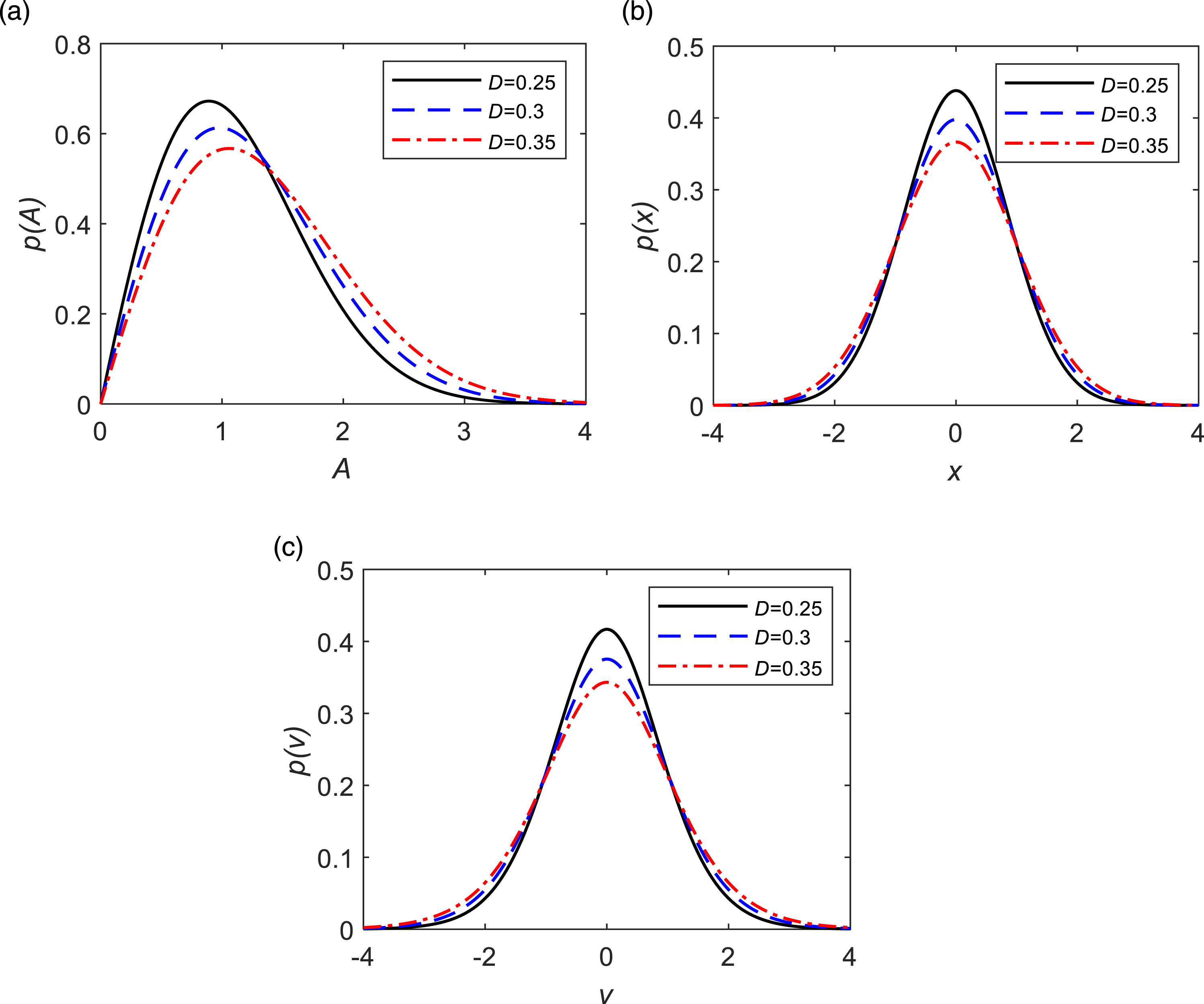
Analyzing the impact of noise intensity on system response via continuous wavelet transform
The simulation parameters remain the same. Figure 16 shows the time history of the system for D = 0.35. By comparing it with Figure 6, it is found that the increase in noise intensity D amplifies the displacement and velocity variations, indicating that the increase in noise intensity exacerbates the vibrations of the system in a stochastic environment. Figure 17 presents the energy distribution of continuous wavelet coefficients for D = 0.35. Due to the change in noise intensity, the random numbers of the stochastic excitation change, resulting in shifts in the positions of energy peaks. Therefore, only the impact of noise intensity on the frequency band is considered. From the frequency domain perspective, it can be seen that the increase in noise intensity does not significantly affect the frequency band, which remains in the range of 0.1–0.3, with the frequency peak still around 0.2. Time-displacement and time-velocity graphs of the system at D = 0.35. (a) Time-Displacement Graph and (b) Time-Velocity Graph. Energy distribution map of continuous wavelet coefficients at D = 0.35. (a) Two-dimensional map of the energy distribution of continuous wavelet coefficients and (b) Three-dimensional map of the energy distribution of continuous wavelet coefficients.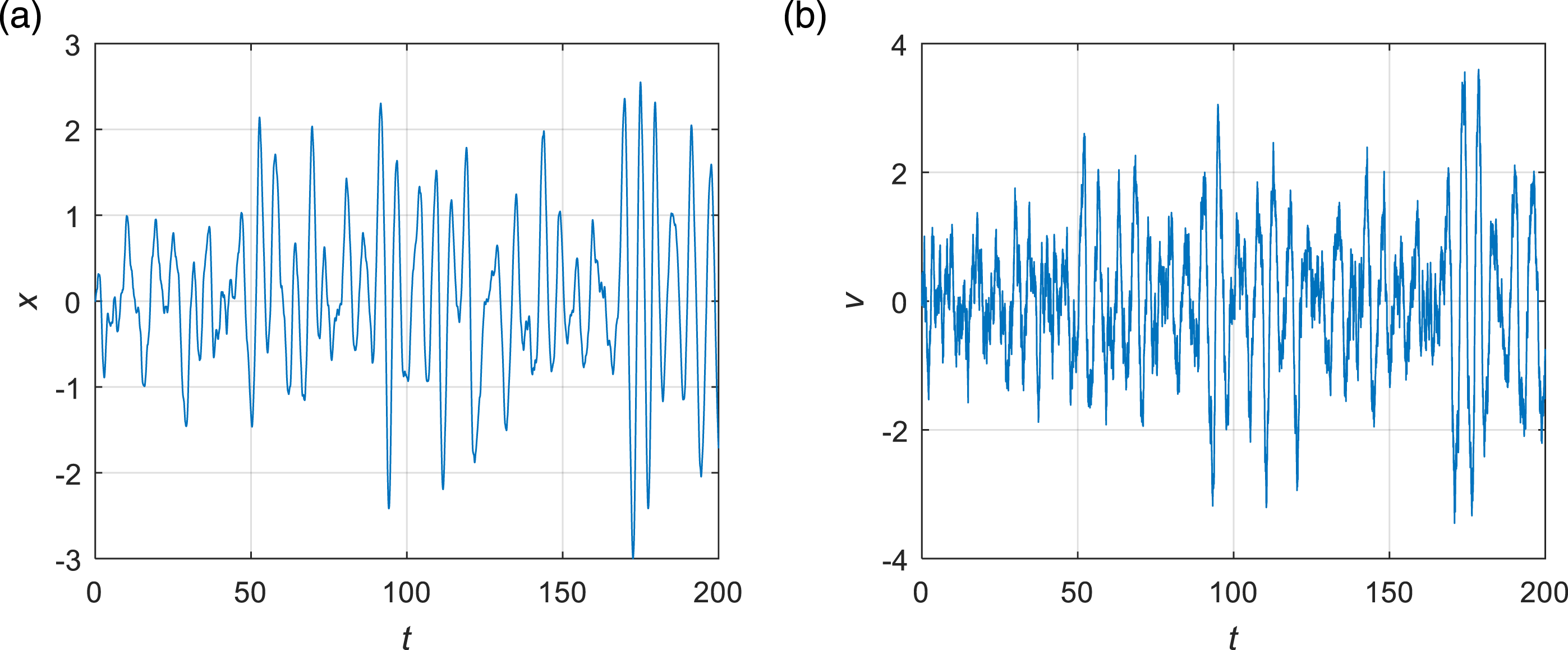
Conclusion
In this paper, we focus on a nonlinear system featuring a Bingham model magneto-rheological damper. We apply the stochastic averaging method to derive its steady-state probability density. Numerical simulations are used for comparison, confirming the accuracy of the analytical results. Building on this, the effects of system viscous damping, Coulomb damping, and noise intensity on the system’s steady-state response were analyzed from both time-domain and frequency-domain perspectives. The study found that: (1) The increase in both system viscous damping and Coulomb damping leads to a rise in the peak values of the steady-state probability density functions of amplitude, displacement, and velocity, as well as the joint probability density function of displacement and velocity. Additionally, it reduces the amplitude in the time-displacement and time-velocity graphs. This indicates that increasing viscous damping and Coulomb damping both suppress system vibrations. In this stochastic model, when the velocity is relatively low, an equal increase in viscous damping and Coulomb damping results in a more significant impact on the system’s steady-state response from Coulomb damping. From a frequency domain perspective, it is observed that increasing viscous damping and Coulomb damping in this system both lead to a reduction in the wavelet transform energy peaks, with the phenomenon of high energy in a single frequency band gradually disappearing and multiple frequency band energy peaks emerging. However, in this system, the reduction in energy peaks is more pronounced with increased Coulomb damping. This finding has important implications for optimizing system damping design and improving its dynamic performance. (2) As the noise intensity increases, the peak values of the probability density function (PDF) for system amplitude, displacement, and velocity significantly decrease. Concurrently, the probability of the system remaining in a balanced state also diminishes. This indicates that the system’s vibration response intensifies with the increase in external noise intensity. However, wavelet analysis reveals that changes in noise intensity have not yet brought about a noticeable impact on the frequency band. In engineering practice, noise, as an environmental factor that can potentially reduce system stability and enhance response, must not be overlooked regarding its impact on the system.
Footnotes
Declaration of conflicting interests
The author(s) declared no potential conflicts of interest with respect to the research, authorship, and/or publication of this article.
Funding
The author(s) disclosed receipt of the following financial support for the research, authorship, and/or publication of this article: The authors are grateful for the support by the Hebei Provincial Central Guidance Local Science and Technology Development Funding Project through Grant No. 246Z1913G and National Natural Science Foundation of China through Grant No. 12072206.