Stationary response of nonlinear Markovian jump system under wide-band random excitation

Abstract

An approximate procedure for predicting the stationary response of a stochastically excited nonlinear Markovian jump system under wide-band random excitation is proposed. Firstly, a weighted-average system in probability can be established to approximate the original one. Then by using the stochastic averaging method, the weighted-average system was reduced to the one described by a one-dimensional averaged Itô equations. The approximate stationary probability densities of the original system are obtained for different jump rules by solving the associated Fokker–Plank–Kolmogorov equation. Finally, an example of Markovian jump Duffing system excited by wide-band random excitation to illustrate the proposed method in detail and the effectiveness of the proposed method is verified via comparing the analytical results with those from Monte Carlo simulation.

Introduction

Markovian jump systems (MJSs) are a class of systems with the Markovian transitions between the 'forms' determined by random abrupt variations in their structures, and they can be used to model a large class of practical systems, such as target tracking systems, manufacturing systems, chemical process, power systems and economic systems. Since Krasosvkii et al. first introduced MJSs in 1960s,^1,2 considerable attention has been devoted to the analysis and synthesis of MJSs.^3–6 Necessary and sufficient conditions for moment stability were obtained by means of an explicit formula for the corresponding Lyapunov exponent for piecewise deterministic jump linear system. ⁷ Kushner ⁸ applied an almost sure stability concept to the jump linear systems. Krasosvkii studied the LQR control of the Markovian jump linear systems. Sworder ⁹ solved the optimal control problem for finite time horizon using maximum principle. The ergodic control problem of MJSs is studied based on the dynamic programming principle. ¹⁰ However, the previous study on MJSs mainly focused on the stability and optimal control.^11–14 Little effort has been made to the research of the response of the MJSs, especially for stochastically excited nonlinear MJSs. Stationary response of nonlinear MJSs excited by Gaussian white noise has been studied by Huan et al. ¹⁵ Development of methodology for analysis of nonlinear MJS is thus much deserving.

In the past two decades, substantial advances have been made in the field of nonlinear vibration. The notable numerical contributions on this subject are the use of harmonic balance method, ¹⁶ multimode approach, ^{17, 18} variational iteration method,¹⁹ homotopy perturbation method. ^{20, 21} On the other hand, the nonlinear structures are often subjected to severe random loadings due to wind, wave, earthquake, etc. In many cases, it is much appropriate to treat random loadings as a wide-band noise with rational spectral density. Considering that the response of the nonlinear system is not a diffusive Markov process, it is difficult to directly apply the theory of diffusive Markov process to solve the response problem. Recently, a stochastic averaging method^22–27 for quasi-Hamiltonian systems has been developed by Zhu and his co-workers. Due to the advantage of approximating the original system by diffusive Markov process, stochastic averaging method has been proved as a powerful technique to deal with the aforementioned difficult situations.

The objective of the present paper is to predict the stationary response of the SDOF nonlinear MJSs excited by external and parametric excitations of wide-band random processes. First a weighted-average system in probability without Markovian jump can be established to approximate the original one. By using stochastic averaging, the averaged Itô equations governing the amplitude envelope for each form are then obtained. And the associated Fokker–Planck–Kolmogorov (FPK) equation is resolved, from which the approximate stationary probabilities for assessing the long-term behavior of the original system for different jump rules are finally obtained.

Formulation of problem

Consider a single degree-of-freedom (SDOF) stochastically excited nonlinear system with Markovian jump

$$\begin{array}{l}\ddot{x}+g(x)=\epsilon f(x,\dot{x},s(t))+{\epsilon }^{1/2}{h}_k(x,s(t)){\xi }_k(t)\\ x(t_0)=x_0,s(t_0)=s_0\end{array}$$

(1)

where $g(x)$ is the nonlinear stiffness; $\epsilon$ is a small parameter; $\epsilon f(x,\dot{x},s(t))$ denotes light Markovian jump damping; ${\epsilon }^{1/2}{h}_k(x,s(t))$ ( $k=1,2,\dots m$ ) represent the Markovian jump coefficients of weakly external and (or) parametric random excitations; ${\xi }_k(t)$ are wide-band stationary and ergodic random processes with zero mean and correlation functions $R_{kl}(\tau )$ or spectral densities $S_{kl}(\omega )$ . $s(t)$ is a continuous-time Markovian jump process representing the model or form in which the system operates. $s(t)$ takes discrete values in a given finite set $S=\{1,2,\dots l\}$ with the transition probability

$$P\{s(t+\Delta t)=j|s(t)=i\}=\{\begin{array}{ll}{\lambda }_{ij}\Delta t+o(\Delta t),\hfill & i\ne j\hfill \\ 1+{\lambda }_{ii}\Delta t+o(\Delta t)\hfill & i=j\hfill \end{array}$$

(2)

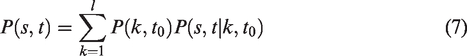
where $P\{s(t+\Delta t)=j|s(t)=i\}$ represents the probability that the system takes the form $j$ at time $t+\Delta t$ given that it has the form $i$ at time $t$ . ${\lambda }_{ij}>0$ for $i\ne j$ is the transition rate from $i$ th form to $j$ th form and

$${\lambda }_{ii}=-\underset{j=1,j\ne i}{\sum ^l}{\lambda }_{ij}$$

(3)

Equation (1) can be used for instance, to model a class of linear or nonlinear systems whose random changes in their structures may be a consequence of abrupt phenomena such as component and/or interconnection failure. Our primary concern here is the stationary response of the system (1).

Stationary probability of $s(t)$

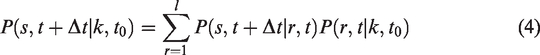
For a continuous-time Markov process, the transition probability of system’s form s(t) satisfies^4,28

$$P(s,t+\Delta t|k,t_0)={\displaystyle \sum _{r=1}^{l}P(s,t+\Delta t|r,t)P(r,t|k,t_0)}$$

(4)

where $P(s,t+\Delta t|r,t)$ is the transition probability defined by equation (2). Substituting equation (3) into equation (4) and letting $\Delta t\to 0$ yields the following Markovian forward equation

$$\frac{\partial P(s,t|k,t_0)}{\partial t}=-{\lambda }_{ss}(t)P(s,t|k,t_0)+{\displaystyle \sum _{u=1,u\ne s}^l{\lambda }_{us}(t)}P(u,t|k,t_0),k,s\in S$$

(5)

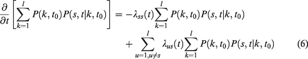
Multiplying both sides of equation (5) by $P(k,t_0)$ and summing $k$ from 1 to l yields

$$\frac{\partial }{\partial t}\left[{\displaystyle \sum _{k=1}^{l}P(k,t_0)P(s,t|k,t_0)}\right]=-{\lambda }_{ss}(t){\displaystyle \sum _{k=1}^{l}P(k,t_0)P(s,t|k,t_0)}+{\displaystyle \sum _{u=1,u\ne s}^l{\lambda }_{us}(t)}{\displaystyle \sum _{k=1}^{l}P(k,t_0)P(s,t|k,t_0)}$$

(6)

For a Markov process, note that

$$P(s,t)={\displaystyle \sum _{k=1}^{l}P(k,t_0)P(s,t|k,t_0)}$$

(7)

Substituting equation (7) into equation (6), equation (6) is reduced as

$$\frac{\partial P(s,t)}{\partial t}=-{\lambda }_{ss}(t)P(s,t)+{\displaystyle \sum _{u=1,u\ne s}^l{\lambda }_{us}(t)P(u,t)}$$

(8)

The initial condition is

$$P(s,t_0)=P_0(s)$$

(9)

The stationary probability of Markovian jump process $s(t)$ can be obtained by letting $\partial P(s,t)/\partial t=0$ as

$$-{\lambda }_{ss}(t)P(s)+{\displaystyle \sum _{u=1,u\ne s}^l{\lambda }_{us}(t)P(u)}=0$$

(10)

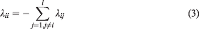
Note that

$${\displaystyle \sum _{u=1}^l{P}_s(u)}=1,P_s(u)\ge 0\text{ for }\text{every}u$$

(11)

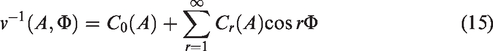
Then, the stationary probability $P_s(u)$ of the Markovian jump process s(t) can be obtained by solving equations (10) and (11).

Averaged equation

In this section, a two-step averaged method is used for original system. First a weighted-average system in probability can be established to approximate the original one. Then a stochastic averaging method is applied to the weighted-average system to transition the system state from rapidly varying of velocity and displacement into the slowly varying form of amplitude.

The first step

Substituting the solved stationary probability $P_s(u)$ into equation (1), a weighted-average system in probability can be obtained as follows

$$\ddot{x}+g(x)=\epsilon {\displaystyle \sum _{u=1}^{l}f(x,\dot{x},u)}{P}_s(u)+{\epsilon }^{1/2}{\displaystyle \sum _{u=1}^l{h}_k(x,u)P_s(u){\xi }_k(t)}$$

(12)

According to the limited averaging principle, ²⁹ as $\epsilon \to \text{0}$ , the solution of the system (12) converges in probability to the solution of system (1). After the weighted averaging, the original system can be approximated by the one without Markovian jump.

The second step

When ε is small, system (12) has periodic random solutions around the trivial solution. The sample solution can be assumed to be in the following form ³⁰

$$x(t)=A\cos \hspace{0.17em}\Phi (t)+B,\dot{x}(t)=-Av(A,\Phi )\sin \hspace{0.17em}\Phi (t),\Phi (t)=\mu (t)+\Theta (t)$$

(13)

where $A$ denotes the amplitude of the oscillator, and

$$v(A,\Phi )=\frac{d\mu }{dt}=\sqrt{\frac{2[U(A+B)-U(A\cos \hspace{0.17em}\Phi +B)]}{A^2{\sin }^2\Phi }}$$

(14)

denotes the instantaneous frequency. $U(x)={\int }_0^{x}g(u)\text{d}u$ is the potential energy. $A,\Phi ,\mu ,\Theta ,v$ are all random processes. $\cos \hspace{0.17em}\Phi (t)$ and $\sin \hspace{0.17em}\Phi (t)$ are called generalized harmonic functions. $v^{-1}(A,\Phi )$ can be expanded into Fourier series

$$v^{-1}(A,\Phi )=C_0(A)+{\displaystyle \sum _{r=1}^{\infty }{C}_r(A)\cos \hspace{0.17em}r\Phi }$$

(15)

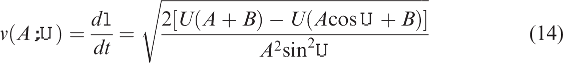
Integrating equation (15) with respect to $\Phi$ from 0 to $2\pi$ yields average period

$$T(A)=2\pi C_0(A)$$

(16)

Treating equation (13) as a generalized van der Pol transformation from $(x,\dot{x})$ to $(A,\Theta )$ , the following differential equations for $A$ and $\Theta$ can be obtained

$$\begin{array}{l}\frac{\text{d}A}{\text{d}t}=\epsilon F_1(A,\Theta ,s(t))+{\epsilon }^{1/2}{G}_{1k}(A,\Theta ,s(t)){\xi }_k(t)\\ \frac{\text{d}\Theta }{\text{d}t}=\epsilon F_2(A,\Theta ,s(t))+{\epsilon }^{1/2}{G}_{2k}(A,\Theta ,s(t)){\xi }_k(t)\end{array}$$

(17)

where

$$F_1=\frac{-A}{g(A+B)(1+h)}{\displaystyle \sum _{u=1}^{l}f(A\cos \hspace{0.17em}\Phi +B,-Av(A,\Phi )\sin \hspace{0.17em}\Phi ,u)}{P}_s(u)v(A,\Phi )\sin \hspace{0.17em}\Phi$$

$$F_2=\frac{-1}{g(A+B)(1+h)}{\displaystyle \sum _{u=1}^{l}f(A\cos \hspace{0.17em}\Phi +B,-Av(A,\Phi )\sin \hspace{0.17em}\Phi ,u)}{P}_s(u)v(A,\Phi )(\cos \hspace{0.17em}\Phi +h)$$

$$G_{1k}=\frac{-A}{g(A+B)(1+h)}{\displaystyle \sum _{u=1}^l{h}_k(A\cos \hspace{0.17em}\Phi +B,u)P_s(u)}v(A,\Phi )\sin \hspace{0.17em}\Phi$$

$$G_{2k}=\frac{-1}{g(A+B)(1+h)}{\displaystyle \sum _{u=1}^l{h}_k(A\cos \hspace{0.17em}\Phi +B,u)P_s(u)}v(A,\Phi )(\cos \hspace{0.17em}\Phi +h)$$

$$h=\frac{\text{d}B}{\text{d}A}=\frac{g(-A+B)+g(A+B)}{g(-A+B)-g(A+B)}$$

(18)

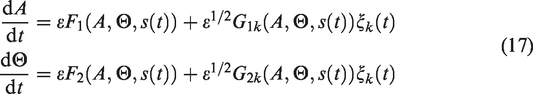
Since $\epsilon$ is a small parameter, the above relation indicates that $A$ is a slowly varying process, while $\Phi (t)$ is a usually rapidly varying process with respect to time. According to the Khasminskii’s theorem, ³¹ $A(t)$ in equation (17) converges weakly to a diffusive Markov process in a time interval of ${\epsilon }^{-1}$ order as $\epsilon \to 0$ . Using the formula in the Khasminskii’s theorem and averaging the drift and diffusion coefficients with respect to $\Phi$ yield the following partially averaged Itô stochastic differential equations.

$$\text{d}A=\epsilon m(A)\text{d}t+{\epsilon }^{1/2}\sigma (A)\text{d}B(t)$$

(19)

where $B(t)$ are standard Wiener processes

$$m(A)={〈F_1+{\displaystyle {\int }_{-\infty }^0\left({\frac{\partial G_{1k}}{\partial A}|}_t{G_{1l}|}_{t+\tau }+{\frac{\partial G_{1k}}{\partial \Theta }|}_t{G_{2l}|}_{t+\tau }\right)}{R}_{kl}(\tau )\text{d}\tau 〉}_{\Phi }$$

$$b(A)={(\sigma (A))}^2={〈{\displaystyle {\int }_{-\infty }^{\infty }({\partial G_{1k}|}_t{G_{1l}|}_{t+\tau })}{R}_{kl}(\tau )\text{d}\tau 〉}_{\Phi }$$

(20)

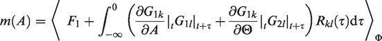
and ${〈.〉}_{\mathrm{\Phi }}$ denotes the averaging operation with respect to $\mathrm{\Phi }$ from 0 to $2\mathrm{\pi }$ , i.e.

$${〈·〉}_{\Phi }=\frac{1}{2\pi }{\displaystyle {\int }_0^{2\pi }(·)}\text{d}\Phi$$

(21)

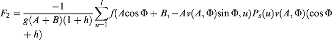
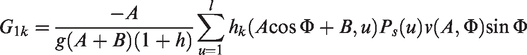
To obtain the explicit expressions for $m(A)$ and $\sigma (A)$ in equation (20), the following steps were taken: first expanding $F_1$ , $G_{ik}$ into Fourier series with respect to Φ, integrating with respect to τ and then averaging with respect to Φ.

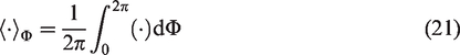
The reduced FPK equations associated with the averaged Itô equations are in the following forms

$$0=-\frac{\partial (m(A)p(A))}{\partial A}+\frac{1}{2}\frac{{\partial }^2(b(A)p(A))}{\partial A^2}$$

(22)

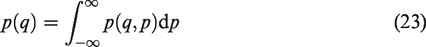
where $p(A)$ is the stationary probability density of the amplitude. $p(A)$ is obtained readily by solving equation (22) using the finite difference method. The stationary probability density $p(q)$ of the generalized displacement is then obtained as

$$p(q)={\displaystyle {\int }_{-\infty }^{\infty }p}(q,p)\text{d}p$$

(23)

where $p(q,p)$ is the stationary joint probability density of the generalized displacement and generalized momenta. It is defined as

$$p(q,p)={\frac{p(H)}{T(H)}|}_{H=H(q,p)},p(H)=p(A)\left|\frac{\text{d}A}{\text{d}H}\right|={\frac{p(A)}{g(A)(1+h)}|}_{A=U^{-1}(H)-B}$$

(24)

is the stationary joint probability density of the generalized displacement and generalized momenta.

Note that rigorous analysis of the errors committed by stochastic averaging has not been reported in the open literature. So, analytical quantification of the errors of the method proposed can only be examined by comparison with direct simulations.

Numerical example

To demonstrate the validity and accuracy of the proposed method, considering a stochastically excited nonlinear oscillator that is capable of independent Markovian jump and governed by

$$\ddot{X}+{\omega }_0^{2}X+\alpha X^3=-c(s(t))\dot{X}+f_1(s(t)){\xi }_1(t)+X{f}_2(s(t)){\xi }_2(t)$$

(25)

where $c(s(t))$ is Markovian jump coefficient of linear damping; $f_i(s(t))$ is Markovian jump coefficient of external and/or parametric random excitation; $s(t)$ is a continuous-time Markov process representing the system's form with the transition probability defined in equation (2). $s(t)$ takes discrete values in a given finite set $S=\{1,2,\dots l\}$ . ${\xi }_i(t)$ are independent stationary and ergodic wide-band noises with zero mean and rational spectral densities

$$S_i\left(\omega \right)=D_i{\left[\pi \left({\omega }^2+{\omega }_i^2\right)\right]}^{-1}\left(i=1,2\right)$$

(26)

${\xi }_i(t)$ can be regarded as the output of Gaussian white noises to the following first-order linear filters

$${\dot{\xi }}_i+{\omega }_i{\xi }_i=W_i\left(t\right),i=1,2$$

(27)

where $W_i(t)$ are Gaussian white noises with intensities $2D_i$ .

For the system (25), the instantaneous frequencies are of the following form

$$v(A,\Phi )={\left[\left({\omega }_0^2+3\alpha A^{\text{2}}/4\right)\left(1+\eta \cos \hspace{0.17em}\left(2\Phi \right)\right)\right]}^{1/2}$$

$$\eta =\left(\alpha A^{\text{2}}/4\right)/\left({\omega }_0^2+3\alpha A^{\text{2}}/4\right)\le 1/3$$

(28)

$v_i(A_i,{\Phi }_i)$ can be approximated by the following finite sum with a relative error less than 0.03%

$$v(A,\Phi )=b_0(A)+b_2(A)\cos \hspace{0.17em}2\Phi +b_4(A)\cos \hspace{0.17em}4\Phi +b_6(A)\cos \hspace{0.17em}6\Phi$$

(29)

where

$$\begin{array}{l}{b}_0\left(A\right)={\left({\omega }_{\text{0}}^{\text{2}}+3\alpha A^{\text{2}}/4\right)}^{1/2}\left(1-{\eta }^{\text{2}}/16\right)\\ b_2\left(A\right)={\left({\omega }_{\text{0}}^2+3\alpha A^{\text{2}}/4\right)}^{1/2}\left(\eta /2+3{\eta }^{\text{3}}/64\right)\\ b_4\left(A\right)={\left({\omega }_{\text{0}}^2+3\alpha A^{\text{2}}/4\right)}^{1/2}\left(-{\eta }^{\text{2}}/16\right)\\ b_6\left(A\right)={\left({\omega }_{\text{0}}^2+3\alpha A^{\text{2}}/4\right)}^{1/2}\left({\eta }^{\text{3}}/64\right)\end{array}$$

(30)

Following the averaging steps in equations (12) to (20), the averaged Itô equation of system (25) with Markovian jump process is obtained

$$\text{d}A=m(A)\text{d}t+\sigma (A)\text{d}B(t)$$

(31)

where $m(A)$ and $\sigma (A)$ are given in Appendix 1.

The associated averaged FPK equation of the Itô equation (31) is

$$-\frac{\partial }{\partial A}[m(A)p(A)]+\frac{1}{2}\frac{{\partial }^2}{\partial A^2}[{\left\{\sigma (A)\right\}}^{2}p(A)]=0$$

(32)

The stationary probability density $p(A)$ can be obtained by solving the associated FPK equation (32) numerically. The stationary probability densities $p(q)$ and $p(q,p)$ are then determined by equations (23) and (24).

Two-form system

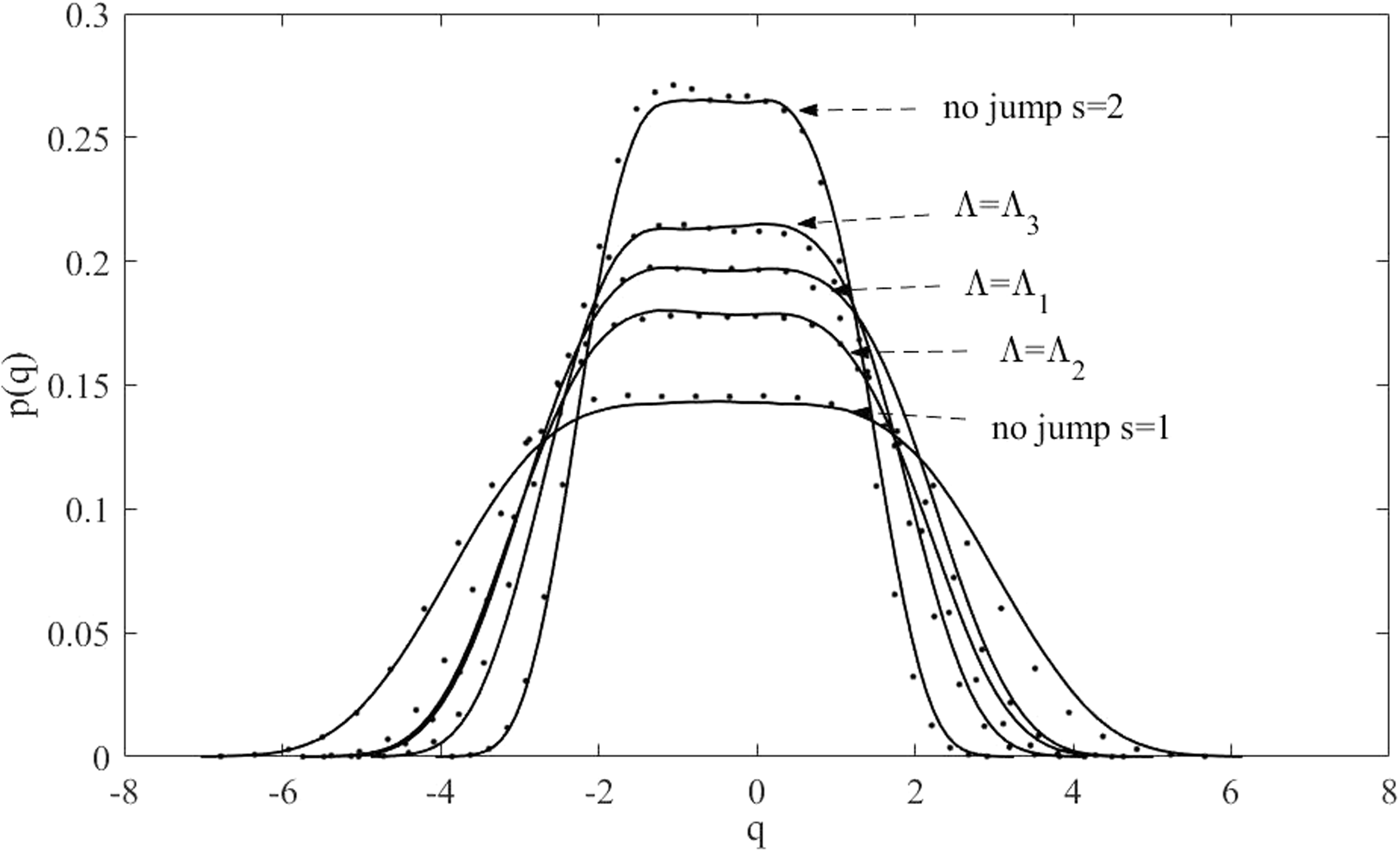
In this case, $l=2$ and $S=\{1,2\}$ . Some numerical results are obtained as shown in Figures 1 to 3 for system parameters: ${\omega }_0=1,$ $\alpha =1,$ ${\omega }_1={\omega }_2=5,$ $D_1=1,$ $D_2=2,$ $c^{(1)}=0.01,$ $c^{(2)}=0.03,$ $f_1^{(1)}=f_2^{(1)}=2,$ $f_1^{(2)}=f_2^{(2)}=1.$ Characterize the transition rate ${\lambda }_{ij}$ between the form $i$ and the form $j$ by a transition matrix $\Lambda =[{\lambda }_{ij}]$ . Three special cases are considered, with

$${\Lambda }_1=\left[\begin{array}{cc}-2& 2\\ 2& -2\end{array}\right],{\Lambda }_2=\left[\begin{array}{cc}-1& 1\\ 2& -2\end{array}\right],{\Lambda }_3=\left[\begin{array}{cc}-2& 2\\ 1& -1\end{array}\right]$$

(33)

The stationary probability density $p(q)$ of displacement is shown in Figure 1, when the transition rates are specified by the three transition matrices in equation (33). The probability densities when Markov jump process is fixed at either $s(t)=1$ or $s(t)=2$ are also plotted. Obviously, when the system operates in the form $s(t)=2$ , it has larger damping coefficients and smaller amplitudes of wide-band excitations than when it operates in the form $s(t)=1$ . There is a higher probability that $p(q)$ will be located near their equilibrium when the system spends more time in the form $s(t)=2$ . Hence, as shown in Figure 1, $p(q)$ has the largest mode around $q=0$ if $s=2$ , and the mode around $q=0$ will decrease as the system cycles through $\Lambda ={\Lambda }_3$ , $\Lambda ={\Lambda }_1$ , $\Lambda ={\Lambda }_2$ and $s(t)=1$ .

Figure 1.

The stationary probability density $p(q)$ of displacement of 2-form system (25) for $\Lambda ={\Lambda }_1$ , $\Lambda ={\Lambda }_2$ , $\Lambda ={\Lambda }_3$ in equation (32), and when the system is fixed at $s(t)=1$ and $s(t)=2$ .

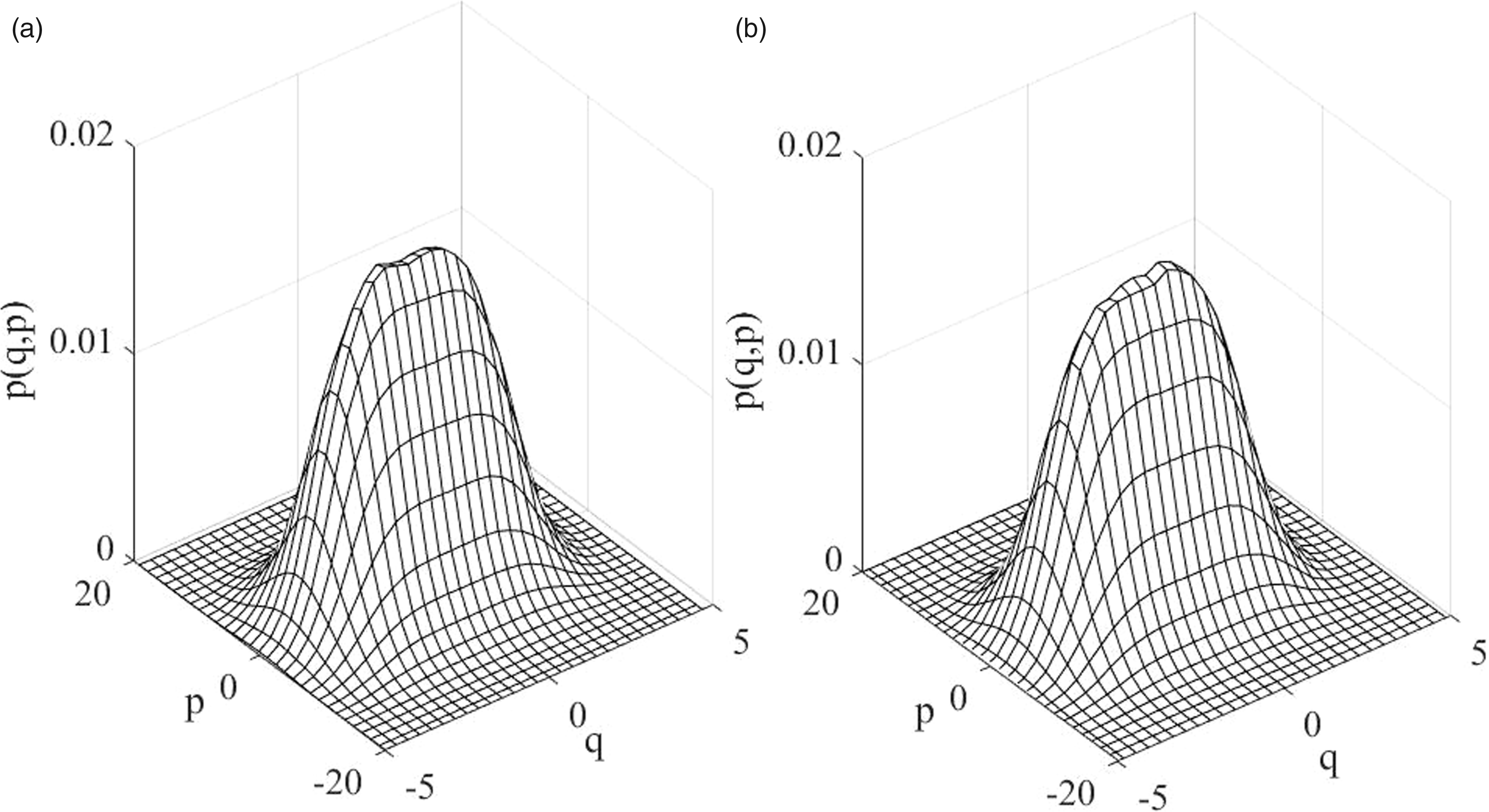
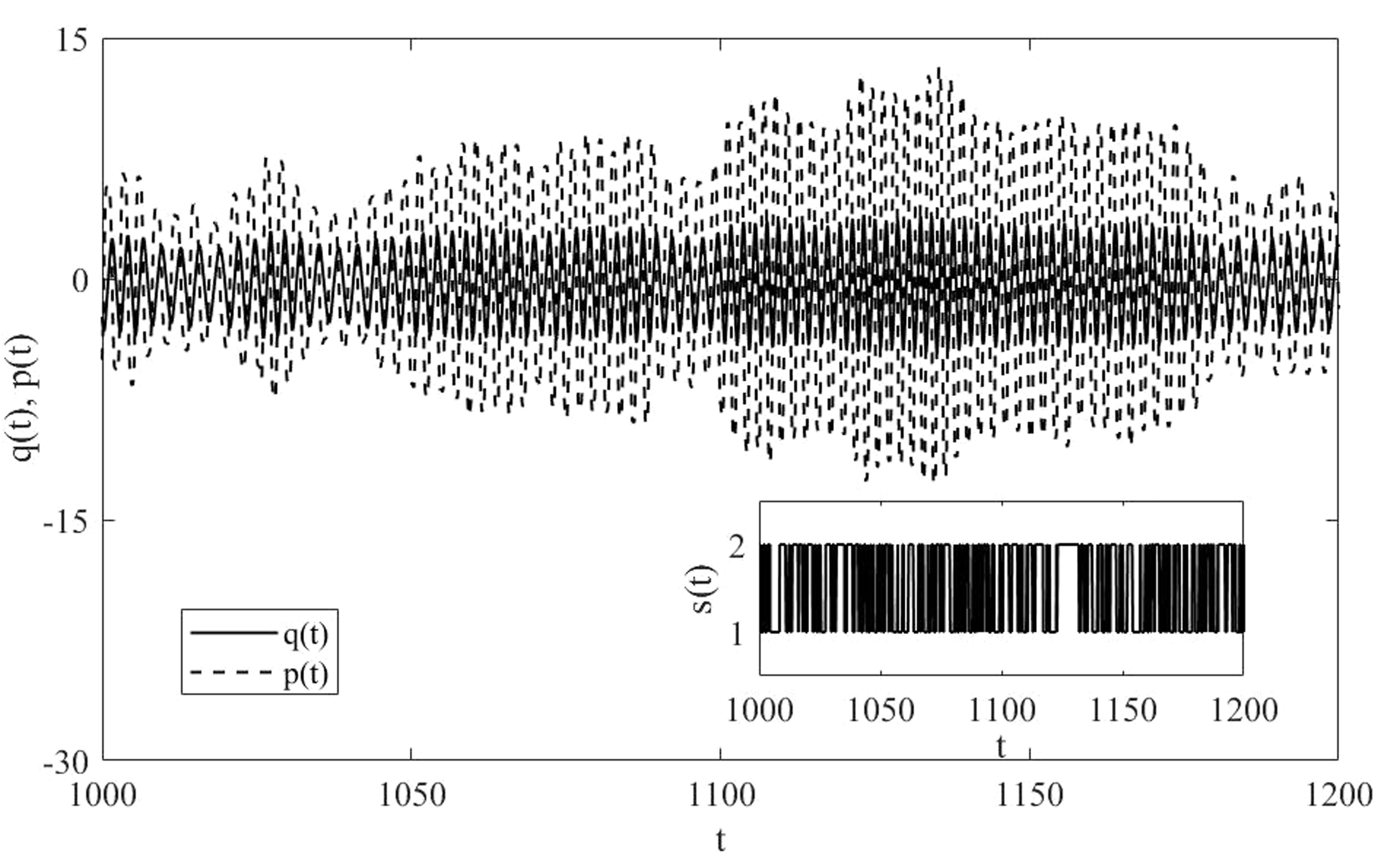
The lines are obtained from solving averaging FPK equation (32), while the dots are obtained by direct simulation of system (25). The joint probability densities $p(q,p)$ of the displacement and momenta obtained from equations (32) and (25) are shown in Figure 2(a) and (b), respectively. Observe that the analytical results agree well with those from digital simulation of original system (25), which demonstrates the validity and accuracy of the proposed method. Finally, a sample time history of the displacement $q$ , momentum $p$ of the system (25), and the jump parameter $s(t)$ for 3-form case are shown in Figure 3.

Figure 2.

The joint probability densities $p(q,p)$ of the displacement and momenta of 2-form system (25) with the transition rates $\Lambda ={\Lambda }_2$ . (a) analytical result; (b) Monte Carlo simulation.

Figure 3.

The sample time history of stationary response of 2-form system (25).

Three-form system

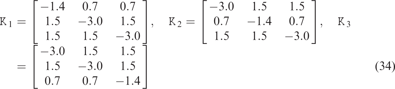
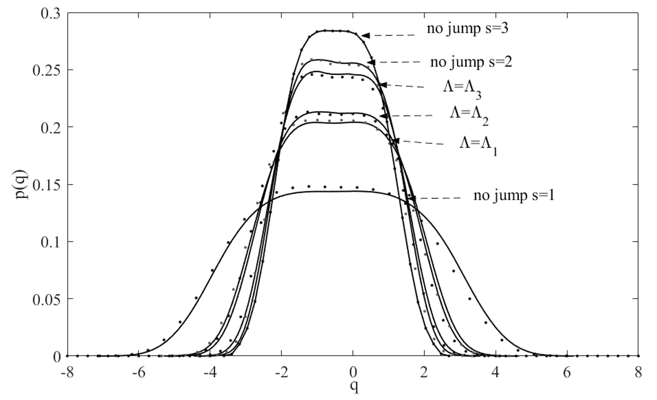
In this case, $l=3$ and $S=\{1,2,3\}$ . The numerical results shown in Figures 4 to 6 are for system with parameters: ${\omega }_0=1,$ $\alpha =1,$ ${\omega }_1={\omega }_2=5,$ $D_1=1,$ $D_2=2,$ $c^{(1)}=0.01,$ $c^{(2)}=0.025,$ $c^{(3)}=0.04,$ $f_1^{(1)}=f_2^{(1)}=2,$ $f_1^{(2)}=f_2^{(2)}=f_1^{(3)}=f_2^{(3)}=1.$ Three special cases are considered, with

$${\Lambda }_1=\left[\begin{array}{ccc}-1.4& 0.7& 0.7\\ 1.5& -3.0& 1.5\\ 1.5& 1.5& -3.0\end{array}\right],{\Lambda }_2=\left[\begin{array}{ccc}-3.0& 1.5& 1.5\\ 0.7& -1.4& 0.7\\ 1.5& 1.5& -3.0\end{array}\right],{\Lambda }_3=\left[\begin{array}{ccc}-3.0& 1.5& 1.5\\ 1.5& -3.0& 1.5\\ 0.7& 0.7& -1.4\end{array}\right]$$

(34)

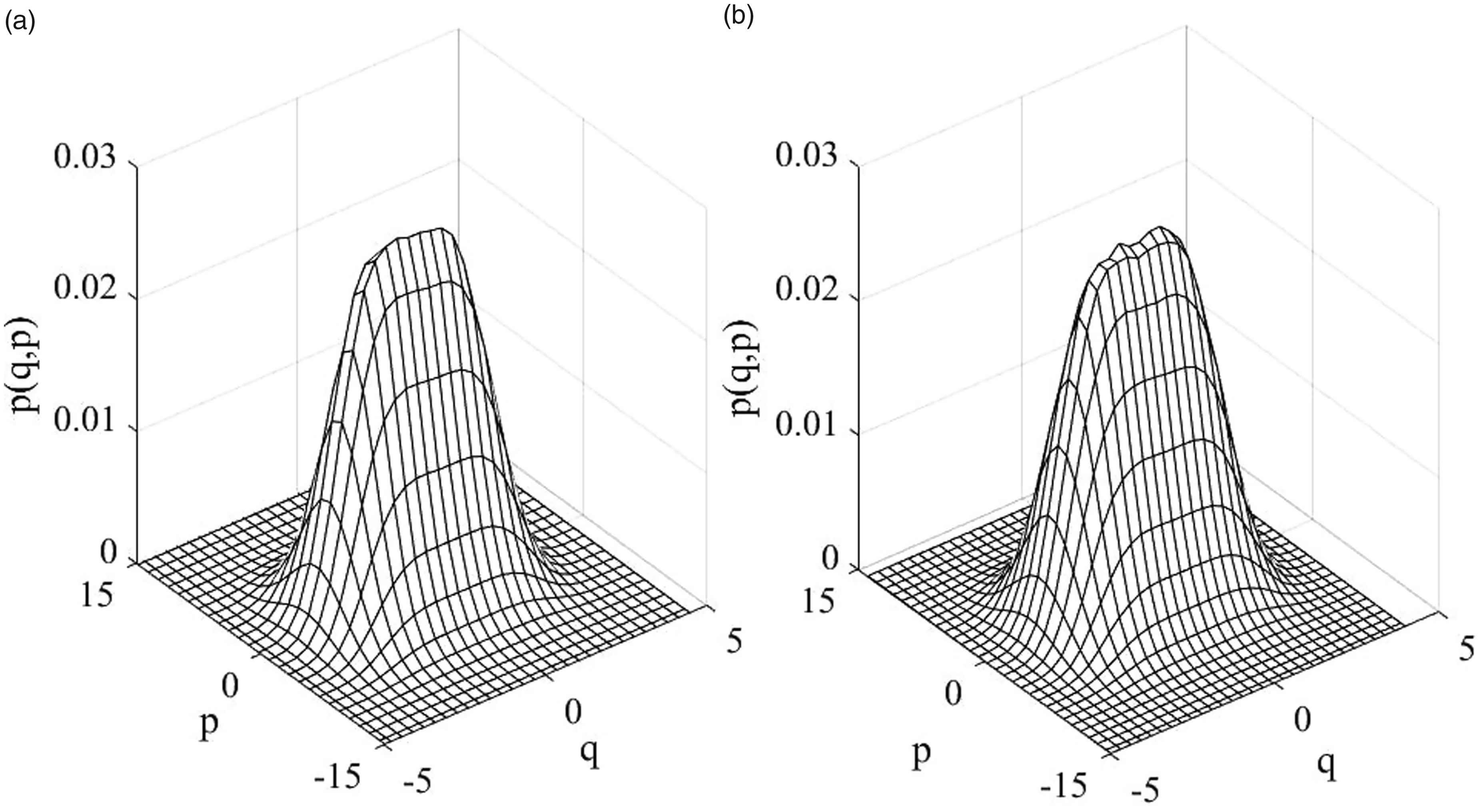
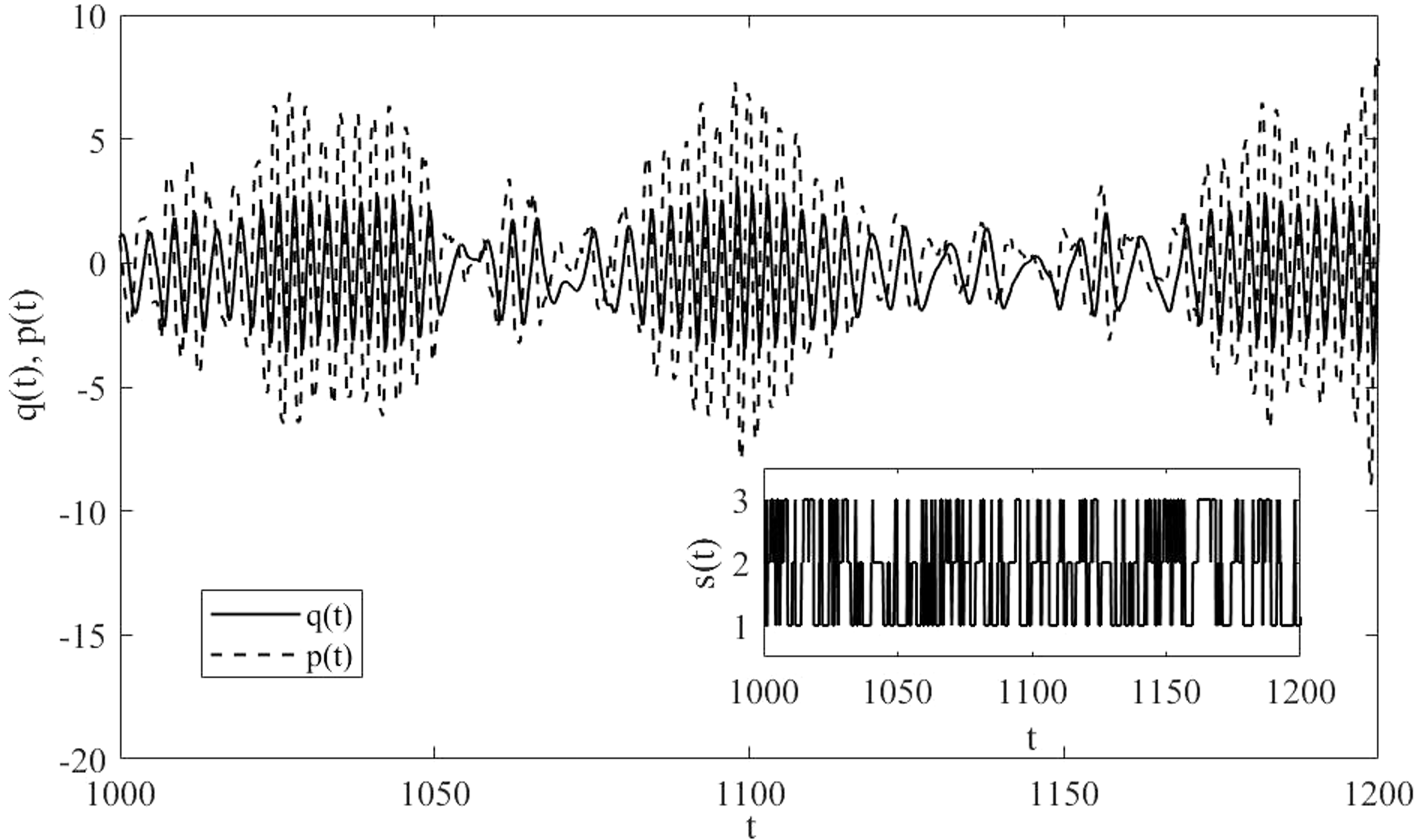
The stationary probability densities $p(q)$ of displacement are evaluated and plotted in Figure 4 for different cases. The joint probability densities $p(q,p)$ of the displacement and momenta are exhibited in Figure 5(a) and (b). The analytical results obtained by using equation (32) match closely with those from digital simulation of original system (25), which indicates that the proposed method is very effective for solving vibration problems of Markovian jump nonlinear system under random excitations. Finally, a sample time history of the displacement $q$ , momentum $p$ of the system (25), and the jump parameter $s(t)$ for 3-form case are shown in Figure 6.

Figure 4.

The stationary probability density $p(q)$ of displacement of 3-form system (25) for $\Lambda ={\Lambda }_1$ , $\Lambda ={\Lambda }_2$ , $\Lambda ={\Lambda }_3$ in equation (32), and when the system is fixed at $s(t)=1$ , $s(t)=2$ and $s(t)=3$ .

Figure 5.

The joint probability densities $p(q,p)$ of the displacement and momenta of 3-form system (25) with the transition rates $\Lambda ={\Lambda }_2$ . (a) analytical result; (b) Monte Carlo simulation.

Figure 6.

The sample time history of stationary response of 3-form system (25).

Conclusions

In this paper, an approximate method for predicting the stationary response of SDOF nonlinear MJS under wide-band random excitation has been proposed. The original system can be reduced to a one-dimensional Itô equation with Markovian jumps based on the stochastic averaging method. So, the associated stationary FPK equation governing the probability densities of displacements and momenta is resolved. The comparison of the analytical results given by the proposed method with those from digital simulation indicates that the proposed method is a feasible procedure for solving random vibration problem of nonlinear MJS. It is noted that the proposed method has the potential to be extended to the Multi-DOF MJSs.