Sage Journals: Discover world-class research

Abstract

When vibrations generated by marine machinery propagate through a ship’s hull into the ocean, they produce low-frequency radiated noise with distinct “acoustic fingerprint” characteristics. This noise, characterized by stable and concentrated energy, long transmission distances, and difficulty in elimination, becomes the primary target for enemy sonar detection. Active vibration isolation serves as a critical method for reducing low-frequency vibrations in ships and enhancing their acoustic stealth performance. However, control challenges persist, including multi-frequency excitation, frequency fluctuation, multi-channel coupling, and slow convergence speed. To address these issues, this paper introduced an innovative multi-channel decentralized decoupling filtered-x least mean square (DMFxLMS) algorithm. Firstly, a recursive least squares identification algorithm with a forgetting factor was proposed, taking into account the characteristics of single-input, multi-output and multi-input, and multi-output control systems, effectively enhancing the algorithm’s convergence speed and control accuracy. Secondly, based on the decentralized decoupling control concept, the multi-channel control system was simplified into parallel single-channel control loops. The control weight coefficient updates were only related to adjacent error signals, significantly reducing the algorithm’s computational complexity. Thirdly, an anti-impact link was designed to improve the algorithm’s robustness, considering the interference caused by other mechanical equipment during the control process. The influence of abnormal error signals in the control weight coefficient correction term was suppressed, and a percentage function was introduced to limit the output signal. Finally, the feasibility and effectiveness of the DMFxLMS algorithm were verified through simulations and experiments. The results demonstrated that the DMFxLMS algorithm achieved significant control effects for both constant frequency line spectrum excitation and frequency fluctuating line spectrum excitation, fulfilling the objective of reducing base vibration. The DMFxLMS algorithm exhibited fast convergence and excellent robustness, making it suitable for practical engineering applications.

Keywords

Active vibration isolation multi-channel decentralized decoupling filtered-x least mean square algorithm anti-impact design low-frequency line spectrum control

Introduction

During the operation of marine machinery equipment, low-frequency vibrations are generated, which propagate through the ship’s hull, producing low-frequency radiated noise. This noise poses a significant threat to the vessel’s acoustic stealth capabilities. Traditional approaches to addressing vibration issues primarily involve passive control methods that do not require external energy input, such as vibration damping, isolation, absorption, suppression, and structural modifications.¹ Passive vibration isolation operates by isolating the vibration source from the controlled object and introducing vibration isolation components in parallel to the vibration transmission path. This method is straightforward to implement and effectively suppresses mid to high-frequency vibration signals. Currently, widely used passive isolation techniques for marine machinery equipment include single-layer, raft, double-layer, and airbag-based systems. However, passive vibration isolation has limitations in low-frequency line spectrum control. Sudden changes in controlled objects can easily lead to control failure, and passive methods inherently lack adaptability.² In contrast to passive vibration isolation, active vibration isolation introduces a secondary vibration source based on the passive isolation foundation. Actuators generate control forces and can respond in real-time to controlled objects, promptly adjusting control signals. Active isolation demonstrates strong robustness and adaptability to external disturbances and system uncertainties.³ Active control involves employing control algorithms to drive actuators, counteracting initial vibrations. The performance of the control algorithm, as the core of active control, determines the overall performance of the control system.

The least mean square (LMS) adaptive algorithm was first introduced by Widrow and Hoff in 1960.⁴ This iterative algorithm utilizes the variance of error signals as its objective function, causing control weight coefficients to iterate along the negative gradient direction of the variance, gradually approximating the optimal solution.⁵ Du and colleagues applied feedforward active control to the field of vibration control, refining the LMS algorithm based on real-world control systems, effectively suppressing radiated noise generated by structural vibrations.⁶ In practical control systems, the output signal does not directly influence the error signal; instead, it undergoes a series of signal conversions and transmissions, forming physical channels referred to as secondary channels.⁷ The presence of secondary channels causes controller weights to deviate from the optimal direction. To counteract the impact of secondary channels on control, they are commonly employed as filtering stages, filtering the reference input signal to form the filtered-x least mean square (FxLMS) algorithm. Research indicates that factors such as the autocorrelation function of the reference input signal, secondary channel modeling accuracy, control filter structure, and algorithm implementation method all contribute to the control system’s convergence speed, stability, and robustness.⁸ Consequently, numerous scholars have developed a series of improved algorithms, including normalized FxLMS,⁹ Newton FxLMS,¹⁰ leaky FxLMS,¹¹ sign FxLMS,¹² momentum FxLMS,¹³ and variable step size FxLMS.¹⁴ In real-world control systems, a single actuator and error signal is insufficient for meeting the demands of vibration active control, necessitating multiple actuators to broaden the noise reduction range and form multi-channel adaptive control algorithms.¹⁵ George and others proposed a modular LMS framework adaptive algorithm for multi-channel LMS filtering, simplifying calculations and enabling multi-channel control.¹⁶ Wang and colleagues introduced a narrowband multi-channel Newton LMS control algorithm that filters line spectrum reference signals through the secondary channel inverse model.¹⁷ This algorithm’s convergence speed remains largely unaffected by multi-channel coupling characteristics.

The actual control system is difficult for a single actuator and error signal to meet the vibration control requirements, and multiple actuators are needed to expand the noise reduction range, that is, a multi-channel adaptive control algorithm (MFxLMS) is formed.¹⁸ MFxLMS algorithm is still based on FxLMS algorithm, the main implementation of centralized control and distributed control.¹⁹ In order to ensure that the controller converges in the correct direction, the traditional adaptive methods are mostly realized through centralized decoupling, but the increase of the number of actuators and sensors will dramatically increase the computational complexity of the algorithm and reduce the stability of the control process.²⁰ The decentralized decoupling control treats each channel as an independent control loop and ignores the coupling between channels, which has the advantages of low complexity and easy implementation, but may cause the controller to converge in the wrong direction, resulting in control divergence.²¹ At present, MFxLMS algorithm still has many limitations: First, the increase in the number of channels leads to a sharp increase in the calculation amount of the algorithm and the delay of the control system; second, the increase in the number of channels makes the modeling of secondary channels more complicated, and increases the influence of secondary vibration sources on reference signals, which is not conducive to obtaining accurate reference signals. Third, the coupling between the secondary channels is serious, which reduces the stability and reliability of the control system.

In summary, researchers both domestically and internationally have made significant progress in the theoretical and experimental aspects of active vibration isolation control algorithms. However, numerous challenges persist when it comes to controlling complex ship mechanical equipment vibrations, where the vibration source exhibits multi-spectral or even fluctuating characteristics in multi-spectral and multi-channel coupling scenarios. To address this, this paper focuses on a double-layer vibration isolation platform for ship mechanical equipment, overcoming bottlenecks such as low accuracy in secondary channel modeling, slow convergence speed, poor stability, and severe channel coupling. We propose the multi-channel decentralized decoupling filtered-x least mean square (DMFxLMS) algorithm under multi-spectral excitation and verify its convergence, stability, and effectiveness through simulation and experimentation. The research findings hold considerable engineering significance for solving low-frequency line spectrum control problems associated with ship mechanical equipment.

Basic FxLMS theory and least squares recursive identification algorithm

Basic FxLMS theory

The feedforward FxLMS control algorithm employs an FIR filter as the controller and uses the LMS algorithm to update filter parameters while filtering the reference signal through the secondary channel.²² For a double-layer isolation system, the single-input single-output (SISO) algorithm structure is shown in Figure 1.

Figure 1.

Feedforward FxLMS algorithm structure.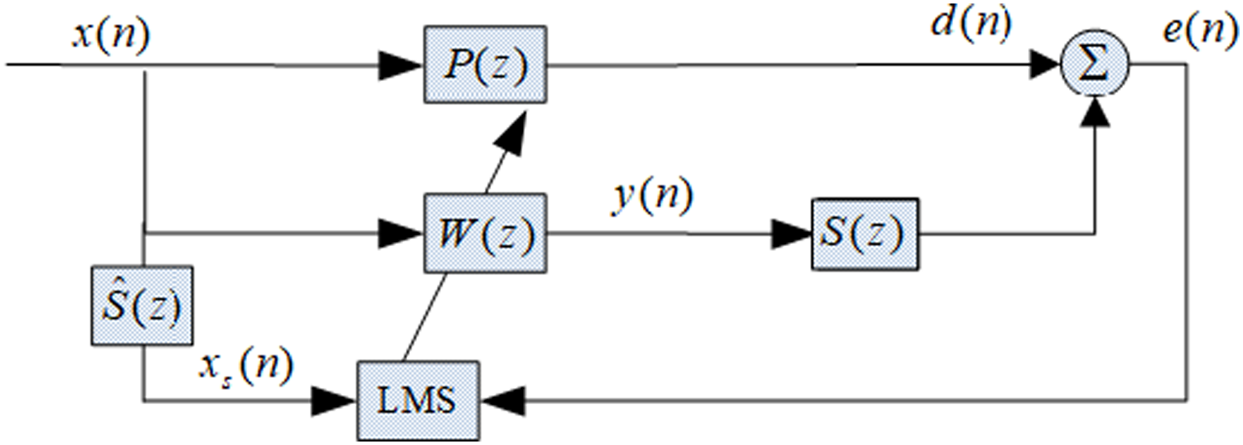

In this structure, $P (z)$ represents the primary channel, $S (z)$ represents the secondary channel, $\hat{S} (z)$ stands for the secondary channel estimation model, and $W (z)$ denotes the controller. $x (n)$ , $x_{s} (n)$ , $y (n)$ , $d (n)$ , and $e (n)$ correspond to the reference signal, filtered reference signal, control output signal, desired signal, and error signal at the time $n$ , respectively.

In the hierarchical controller structure, the variable $w_{i} (i = 0, 1, \dots, L - 1)$ corresponds to the weight coefficient associated with each individual stage of the controller, which comprises L distinct stages in total.²³ The delay unit within the system is represented by the delay operator, denoted as $z^{- 1}$ . As a result, the expression for a delay of one sampling point, symbolized by $x (n)$ , can be described in the following manner:

z^{- 1} x (n) = x (n - 1)

(1)

At this point, both the input signal and controller filter weights can be represented in vector form, that is:

x (n) = {[x (n), x (n - 1), . . . x (n - L + 1)]}^{T}, W (n) = {[w_{0}, w_{1}, . . . w_{L - 1}]}^{T}

(2)

The filter output signal can be expressed as:

y (n) = \sum_{i = 0}^{L - 1} w_{i} x (n - i) = W (z) x (n)

(3)

where

W (z) = w_{0} + w_{1} z^{- 1} + w_{2} z^{- 2} + . . . + w_{L - 1} z^{- (L - 1)}

In the FxLMS algorithm structure, the control output signal $y (n)$ acts on the passive point through the secondary channel, and after superimposing it with the desired signal, it forms the error signal. To facilitate analysis, the secondary channel transfer function is modeled using an M-stage FIR filter, meaning $S (z)$ can be expressed as:

S (z) = s_{0} + s_{1} z^{- 1} + s_{2} z^{- 2} + . . . + s_{M - 1} z^{- (M - 1)}

(4)

The control system error signal $e (n)$ can be written as:

e (n) = d (n) + S (z) y (n)

(5)

Substituting equation (3) into equation (5), denote $x_{s} (n) = S (z) x (n)$ as the reference signal filtered through the secondary channel. In the process of control law design, the error signal $J (n) = {[e (n)]}^{2} / 2$ is employed as the objective function, and the relationship surface of the objective function $J (n)$ concerning the control weight coefficient $w_{i}$ is denoted as the error performance surface. For stationary random signals, the autocorrelation function R of the reference signal constitutes a positive definite matrix. In this case, the error performance surface exhibits a bowl-shaped configuration with a singular minimum point. By computing the first-order derivative of $J (n)$ with respect to the weight coefficient, the optimal control weight coefficient that yields the minimum mean square error is:

W_{o} = R^{- 1} P, R = E [x_{s} (n) x_{s}^{T} (n)], P = E [d (n) x_{s}^{T} (n)]

(6)

In real-world applications of adaptive control systems, it proves challenging to directly calculate the first-order statistical characteristics of signals, particularly when the reference signal undergoes dynamic variations, rendering the optimal solution unattainable.²⁴ In engineering implementations, recursive estimation techniques are typically utilized to progressively converge toward the optimal solution.

According to the gradient descent principle, the adaptive controller’s weight coefficient is updated as follows.

W (n + 1) = W (n) - u \nabla J

(7)

\nabla J

represents the first-order derivative of the objective function with respect to the control weight coefficient and

u

represents the convergence coefficient.

\nabla J = \frac{\partial J (n)}{\partial W (n)} = e (n) \frac{\partial [d (n) + \sum_{i = 0}^{L - 1} w_{i} x_{s} (n - i)]}{\partial w_{i} (i = 0, 1, . . . L - 1)} = e (n) x_{s} (n)

(8)

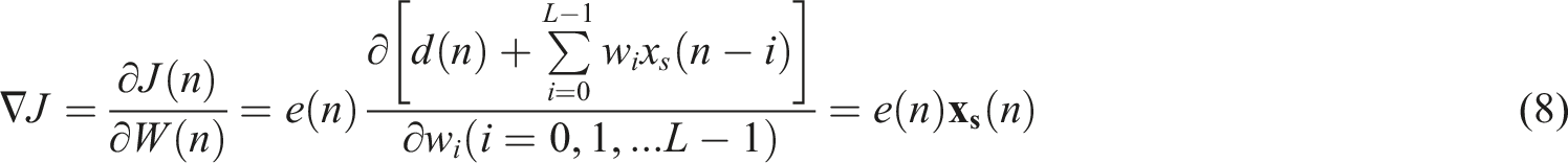
Substituting equation (10) into equation (9) yields the control weight coefficient update formula:

W (n + 1) = W (n) - u e (n) x_{s} (n)

(9)

where u is the iteration step size, and

x_{s} (n)

is the reference signal vector form, which can be written as.

x_{s} (n) = {[x_{s} (n), x_{s} (n - 1), . . . x_{s} (n - L + 1)]}^{T}

(10)

In practical control systems, the secondary channel transfer function cannot be precisely calculated; its estimated value

\hat{S} (z)

, obtained through secondary channel identification, is used for reference signal filtering. The convolution expression is as follows.

x_{s} (n) = \hat{S} (z) x (n) = \sum_{i = 0}^{M - 1} {\hat{s}}_{i} x (n - i)

(11)

Equations (3), (9), and (11) represent the update formulas for the controller output signal, control filter weight coefficient, and filtered reference signal, respectively, constituting the basic FxLMS algorithm.

Recursive least squares identification algorithm

Algorithm principle

In control systems, the controller output signal does not act directly upon the error signal. Instead, they are interconnected through a physical channel composed of elements such as a D/A board, junction box, power amplifier, cable, actuator, error sensor, and A/D board, collectively referred to as the secondary channel. The transfer function is challenging to calculate precisely, necessitating secondary channel identification to obtain its estimated value for reference signal filtering.²⁵ The identification accuracy directly influences the control algorithm’s convergence speed and the steady-state error.

Assuming there is an identification error $Δ S (z)$ in the secondary channel, which is:

\hat{S} (z) = S (z) + Δ S (z)

(12)

The filtered reference signal can be represented as follows:

{\hat{x}}_{s} (n) = x_{s} (n) + Δ x_{s} (n)

(13)

In this context,

Δ x_{s} (n) = Δ S (z) x (n)

denotes the identification error vector of the filtered reference signal. The autocorrelation matrix

\hat{R}

of the filtered reference signal is:

\begin{array}{l} \hat{R} = E [{\hat{x}}_{s} (n) {\hat{x}}_{s}^{T} (n)] = E [(x_{s} (n) + Δ x_{s} (n)) (x_{s}^{T} (n) + Δ x_{s}^{T} (n))] \\ = R + 2 E [Δ x_{s} (n) x_{s}^{T} (n)] + E [Δ x_{s} (n) Δ x_{s}^{T} (n)] \end{array}

(14)

As indicated by equation (16), the presence of identification error results in an increase in the trace of the autocorrelation matrix $\hat{R}$ for the filtered reference signal. Consequently, identification errors significantly affect the convergence and control performance of the algorithm. In cases where the phase angle of the identification error exceeds 90°, the algorithm fails to converge, regardless of the chosen iterative step size. Therefore, precise identification of the secondary channel is an essential prerequisite for implementing the control algorithm.²⁶

For secondary channels characterized by simple parameters, low nonlinearity, and relatively stable performance, finite impulse response (FIR) filters are commonly employed for offline modeling. As FIR filters are finite impulse response filters, they do not necessitate feedback or past outputs, thereby offering non-recursive properties, robust versatility, and other advantages.²⁷ Their straightforward structure is easy to implement and can effectively carry out secondary channel identification. In accordance with the secondary channel definition, when utilizing FIR filters for modeling and analysis, the controller output signal acts as the input to the identification filter, the error signal serves as the desired output signal of the identification filter, and the filter order is denoted by M, then:

e_{a} (k) = \sum_{m = 0}^{M - 1} {\hat{s}}_{m} y (k - m) = \hat{S} (z) y (k)

(15)

where

\hat{S} = {[{\hat{s}}_{0}, {\hat{s}}_{1}, . . . {\hat{s}}_{M - 1}]}^{T}

represents the identification filter weight vector, and

e_{a} (k)

represents the estimated output signal of the identification filter at time k.

The estimated output obtained from the kth observation can be expressed as:

e_{a} (k) = y^{T} (k) \hat{S} + ε (k)

(16)

where

y (k) = {[y (k), y (k - 1), y (k - 2), . . . x (y - M + 1)]}^{T}

and

ε (k)

are random error. The identification residual of the filter at the time k is denoted as:

f_{c} (k) = e (k) - e_{a} (k)

(17)

The estimated output vector for the first K observations can be represented as:

E_{a} = Y^{T} \hat{S} + ε

(18)

E_{a}

represents the estimated output vector,

Y

represents the input signal matrix, and

ε

represents the random error matrix.

\begin{array}{l} E_{a} = {[e_{a} (1), e_{a} (2), . . . e_{a} (K)]}^{T} \\ Y = [\begin{array}{l} y (1) & y (0) & y (- 1) & . . . & y (2 - M) \\ y (2) & y (1) & y (0) & . . . & y (3 - M) \\ . . . & . . . & . . . & . . . & . . . \\ y (K) & y (K - 1) & y (K - 2) & . . . & y (K - M + 1) \end{array}] \end{array}

(19)

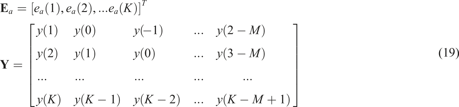
For the first K observations, the performance index is given by:

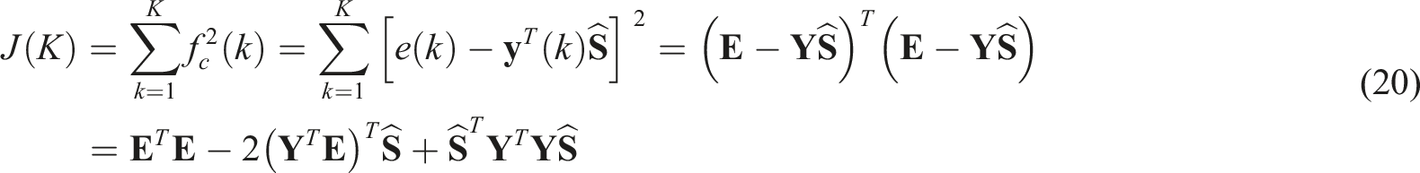
\begin{array}{l} J (K) = \sum_{k = 1}^{K} f_{c}^{2} (k) = \sum_{k = 1}^{K} {[e (k) - y^{T} (k) \hat{S}]}^{2} = {(E - Y \hat{S})}^{T} (E - Y \hat{S}) \\ = E^{T} E - 2 {(Y^{T} E)}^{T} \hat{S} + {\hat{S}}^{T} Y^{T} Y \hat{S} \end{array}

(20)

The weight vector least square estimate corresponds to the weight vector when the performance function takes its minimum value. Taking the first derivative of the performance function, it can be obtained:

{\hat{S}}_{l s} = {(Y^{T} Y)}^{- 1} Y^{T} E

(21)

The value of ${\hat{S}}_{l s}$ represents the minimum least squares estimation of the weight vector. This data processing method adopts a one-shot algorithm, which has a relatively simple theoretical study, but it involves matrix inversion and requires recalculation with each additional observation value. In engineering applications, the weight vector is usually updated using the recursive least squares algorithm.

{\begin{cases} \hat{S} (k + 1) = \hat{S} (k) + Z (k + 1) [e (k + 1) - y^{T} (k + 1) \hat{S} (k)] \\ Z (k + 1) = \frac{P (k) y^{T} (k + 1)}{1 + y^{T} (k + 1) P (k) y (k + 1)} \\ P (k + 1) = P (k) - Z (k + 1) y^{T} (k + 1) P (k), P (k) = {(Y_{k}^{T} Y_{k})}^{- 1} \end{cases}

(22)

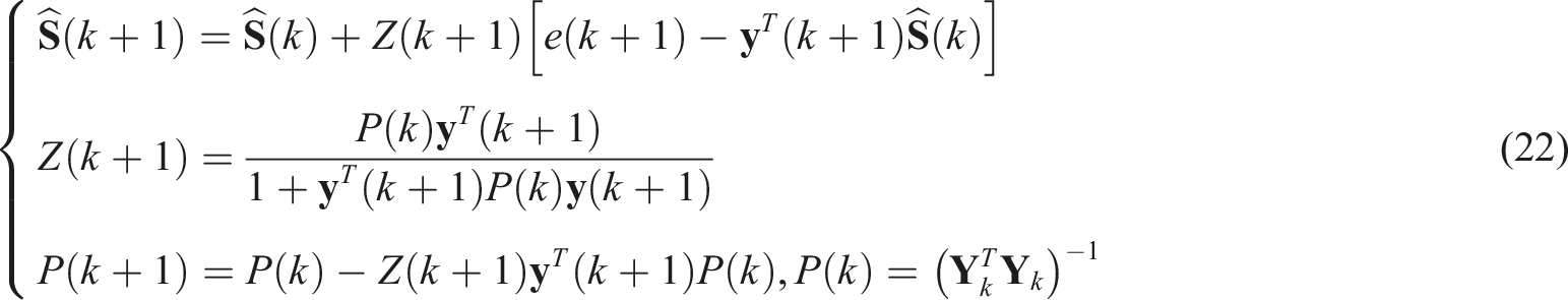
The equation mentioned above represents the weight vector update formula for the recursive least squares (RLS) algorithm.²⁸ However, as the number of observation values increases, there is a possibility of encountering the phenomenon of “data saturation,” where $Z (k)$ and $P (k)$ become increasingly smaller, losing the ability to modify the weight vector and thus, failing to perform the parameter identification. To overcome this issue, a forgetting factor $γ$ is introduced, which acts as a time-varying weighting of the data.²⁹ The most recent data is given a weight of 1, while data from the previous k sampling periods is weighted by $γ^{k}$ . As a result, the weight vector update formula becomes:

{\begin{cases} \hat{S} (k + 1) = \hat{S} (k) + Z (k + 1) [e (k + 1) - y^{T} (k + 1) \hat{S} (k)] \\ Z (k + 1) = \frac{P (k) y^{T} (k + 1)}{γ + y^{T} (k + 1) P (k) y (k + 1)} \\ P (k + 1) = [I - Z (k + 1) y^{T} (k + 1)] P (k) / γ \end{cases}

(23)

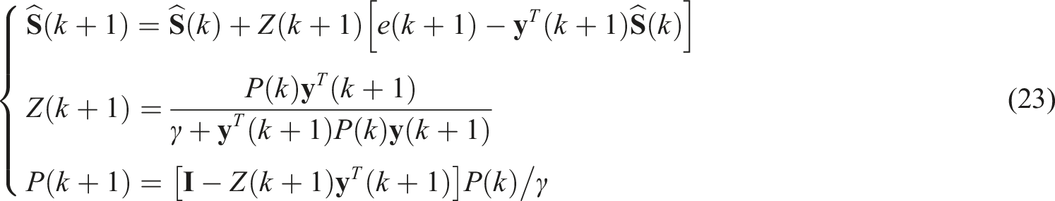
A block diagram showing the identification process is shown in Figure 2. The introduction of the forgetting factor enhances the RLS algorithm’s capability to identify changes in the parameters of secondary channel systems, making it an ideal candidate for use in online identification algorithms for secondary channels. The forgetting factor works by reducing the impact of older data, and it must be a positive number close to 1, neither too large nor too small. If it is too large, the decay effect will be lost and even accelerate the “data saturation” process, while if it is too small, it will result in significant fluctuations in the identified parameters.

Figure 2.

The block diagram of identification process. (a) Identification process. (b) Convergence process of the weight. (c) Result of the secondary channel.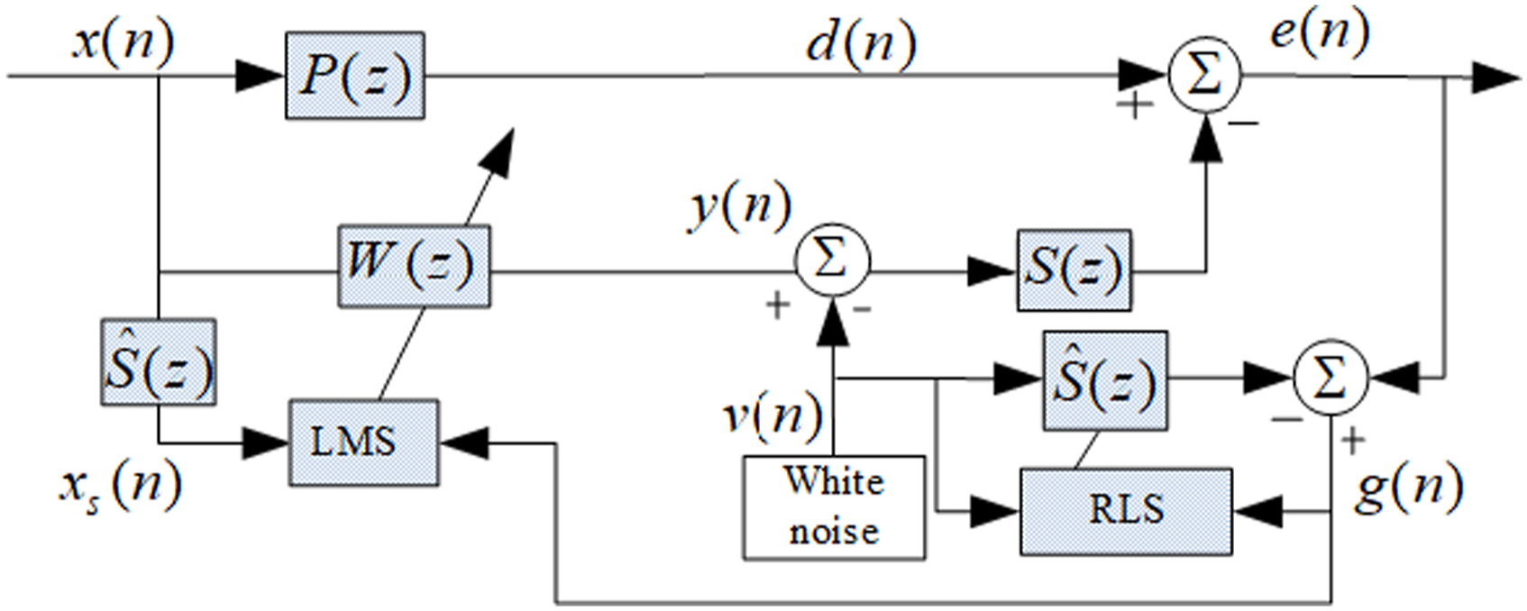

Numerical simulation

In order to establish the validity of the recursive least squares (RLS) identification algorithm incorporating a forgetting factor, a simulation analysis was conducted on a two-layer vibration control system using MATLAB/Simulink. The power spectral decay of the intermediate acceleration signal, before and after control, was employed as the evaluation criterion to objectively reflect the accuracy of the identification algorithm through its control effectiveness.

L_{D} = 10 \lg (\sum d^{2} (n)) - 10 \lg (\sum e^{2} (n))

(24)

Initially, the secondary channel underwent offline identification, in which it was excited using Gaussian white noise with zero mean and a standard deviation of 0.05. The expected value of the secondary channel output was thus obtained, and the RLS identification algorithm incorporating a forgetting factor was utilized to perform modeling analysis and estimate the secondary channel model. Subsequently, the estimated model was introduced into the main control circuit, with the reference signal set as a 37 Hz sine wave overlaid with random noise having a signal-to-noise ratio of 30 dB. The control was executed using the fast and affine projection (FxLMS) algorithm, and the power spectral decay of the error signal, before and after control, was monitored.

The results of the offline identification of the secondary channel using the RLS algorithm with forgetting factor $γ = 0.98$ are shown in Figure 3.

Figure 3.

Results of the RLS algorithm identification. (a) Identification process. (b) Convergence process of the weight. (c) Result of the secondary channel.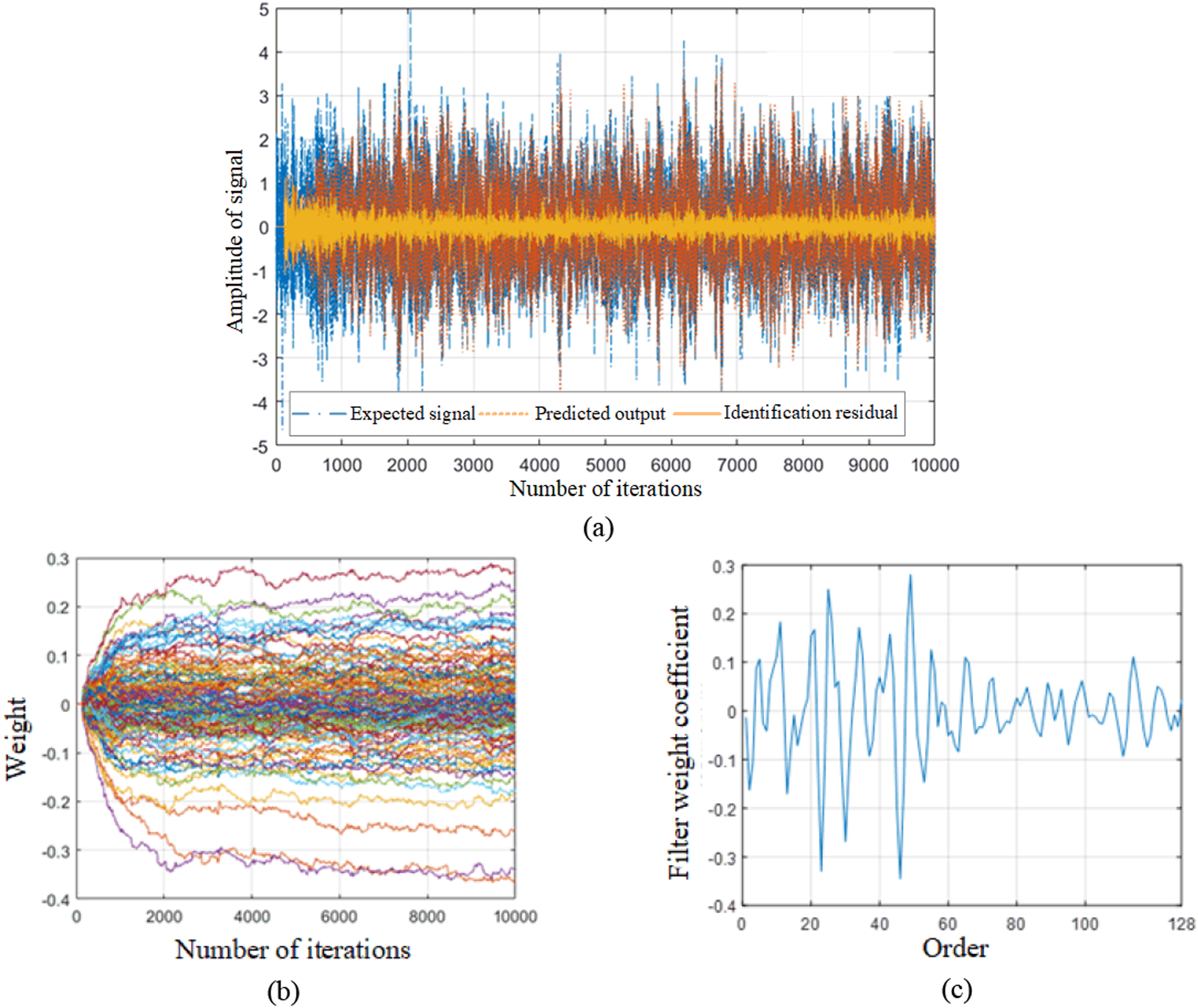

As depicted in Figure 3(a), the expected signal, the predicted output, and the identification residual signal are displayed. The residual signal, after convergence of the identification process, can be seen to be only 8% of the original expected signal amplitude, which is believed to result from electromagnetic interference and the finite number of stages in the FIR filter. The convergence process of the weight vector of the identification filter is shown in Figure 3(b), with a 128th order and reaching a basic convergence after 2000 iterations. The final estimated model of the secondary channel is displayed in Figure 3(c), which was utilized for simulation control. The simulation was executed at a sampling frequency of 1 KHz, with a control iteration step of 5 × 10⁻⁵, and a control order of 200. The error signal before and after control is depicted in Figure 4.

Figure 4.

Effect of active control under the RLS identification algorithm. (a) Time course diagram of the error signal. (b) Power spectrum of the error signal before and after control.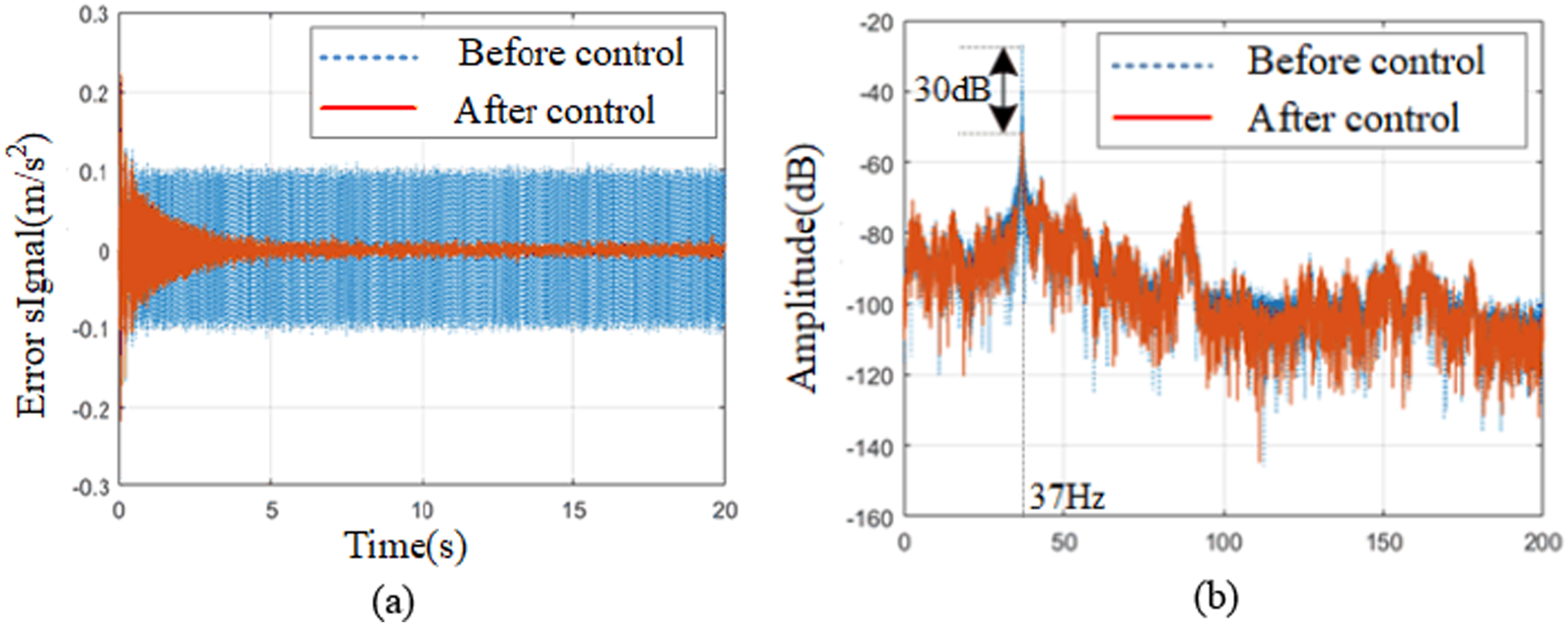

As can be seen from the figure, the error signal decay is apparent after control, and the convergence speed is relatively fast. The peak level drop at 37 Hz reaches 30 dB, and the control effect is significant, objectively reflecting the accuracy of the secondary channel identification.

Multi-channel decentralized FxLMS algorithm and design of anti-shock circuit

Multi-channel decentralized FxLMS algorithm

In practical control systems, it is often difficult to meet the requirements of vibration control with a single actuator and error sensor. Typically, multiple actuators and error sensors are needed to reduce the overall vibration, that is, multi-channel adaptive filtering control algorithms (multi-channel filtered-x least mean square, MFxLMS). Although the algorithm has no essential difference from the single-channel control algorithm, the increase in the number of channels causes a drastic increase in the calculation of the algorithm and the coupling of the secondary channels seriously reduces the stability of the system. Therefore, the implementation of multi-channel control algorithms requires breakthroughs in the following difficulties: (1) The coupling of the secondary channels is serious, and the update of any control filter requires all error signals, with a large amount of calculation and poor stability; (2) when impacted by other equipment during the control process, it can cause an error signal in one channel to be too large, causing the output signal to be almost saturated or overflow, and the algorithm to diverge.³⁰

A multi-channel control system contains a reference signal, N actuators, and N error signals, as shown in Figure 5. Where $P_{i} (z)$ is the ith primary channel; $S_{i j} (z)$ is the secondary channel between the ith actuator and the jth error signal; ${\hat{S}}_{i j} (z)$ is the corresponding estimated identification model; $W_{i} (z)$ is the ith controller; and $y_{i} (n)$ , $d_{i} (n)$ , and $e_{i} (n)$ are the control output signal, expected signal, and error signal corresponding to the ith channel at time n, respectively.

Figure 5.

The algorithm structure of the multi-channel adaptive.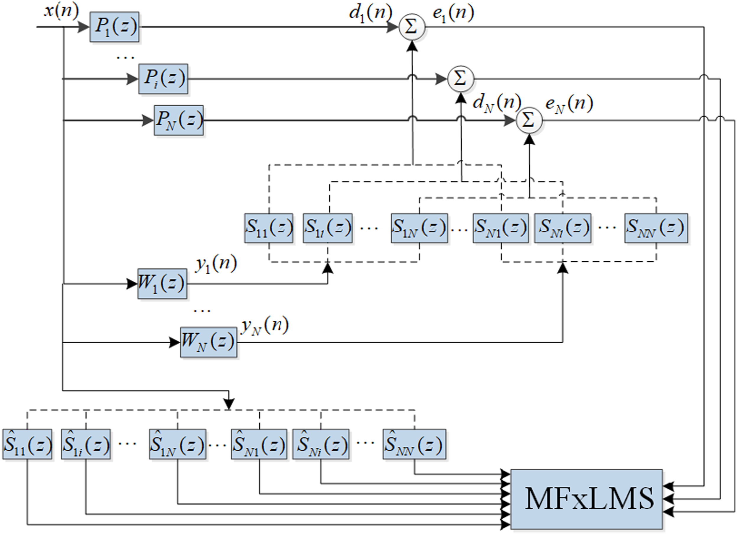

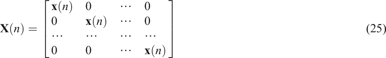
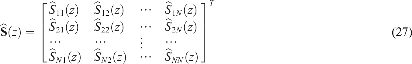
In the multi-channel control system, signals are typically manipulated in the form of matrices or vectors. The reference signal matrix can be expressed as follows:

X (n) = [\begin{array}{l} x (n) & 0 & \dots & 0 \\ 0 & x (n) & \dots & 0 \\ \dots & \dots & \dots & \dots \\ 0 & 0 & \dots & x (n) \end{array}]

(25)

where

x (n) = {[x (n), x (n - 1), \cdot \cdot \cdot, x (n - L + 1)]}^{T}

L

denotes the order of the control filter, the secondary channel transfer function matrix and its corresponding estimation model is given by:

S (z) = {[\begin{array}{l} S_{11} (z) & S_{12} (z) & \dots & S_{1 N} (z) \\ S_{21} (z) & S_{22} (z) & \dots & S_{2 N} (z) \\ \dots & \dots & ⋮ & \dots \\ S_{N 1} (z) & S_{N 2} (z) & \dots & S_{N N} (z) \end{array}]}^{T}

(26)

\hat{S} (z) = {[\begin{array}{l} {\hat{S}}_{11} (z) & {\hat{S}}_{12} (z) & \dots & {\hat{S}}_{1 N} (z) \\ {\hat{S}}_{21} (z) & {\hat{S}}_{22} (z) & \dots & {\hat{S}}_{2 N} (z) \\ \dots & \dots & ⋮ & \dots \\ {\hat{S}}_{N 1} (z) & {\hat{S}}_{N 2} (z) & \dots & {\hat{S}}_{N N} (z) \end{array}]}^{T}

(27)

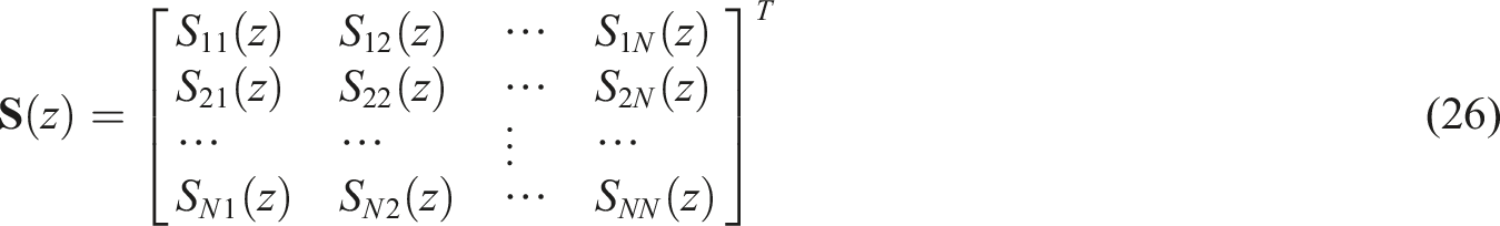
The estimation models for the secondary channels are all M-order FIR filters, and any estimation model ${\hat{S}}_{i j} (z)$ can be represented as:

{\hat{S}}_{i j} (z) = {\hat{S}}_{i j 1} + {\hat{S}}_{i j 2} z^{- 1} + {\hat{S}}_{i j 3} z^{- 2} + . . . + {\hat{S}}_{i j M} z^{- (M - 1)}

(28)

The controller weight coefficient matrix is:

W (n) = {[w_{1} (n), w_{2} (n), . . . w_{N} (n)]}^{T}

(29)

where

w_{i} (n) = {[w_{i 1} (n), w_{i 2} (n) . . . w_{i L} (n)]}^{T}

The output signal is given by:

Y (n) = {[y_{1} (n), \cdot \cdot \cdot, y_{N} (n)]}^{T} = X (n) W (n)

(30)

From Figure 5, it can be inferred that the error signal is:

E (n) = {[e_{1} (n) e_{2} (n) \cdot \cdot \cdot e_{N} (n)]}^{T} = D (n) + S (z) Y (n)

(31)

where

D (n)

is the expected signal. In component form, it can be expressed as:

e_{k} (n) = d_{k} (n) + \sum_{i = 1}^{N} S_{i k} (z) y_{i} (n) = d_{k} (n) + \sum_{i = 1}^{N} S_{i k} (z) w_{i} (n) x (n)

(32)

At this stage, the objective function of the multi-channel control algorithm is the sum of all the error signals.

J (n) = E^{T} (n) E (n) = \sum_{k = 1}^{N} e_{k}^{2} (n)

(33)

Applying the steepest descent principle, the iterative update algorithm for the control filter can be expressed in component form as follows:

w_{k} (n + 1) = w_{k} (n) - μ_{k} (n) \sum_{i = 1}^{N} {\hat{x}}_{i k} (n) e_{i} (n) (k = 1, 2, \cdot \cdot \cdot, N)

(34)

where

{\hat{x}}_{i k} (n)

represents the reference signal filtered by the secondary channel estimation model

{\hat{S}}_{i k} (z)

and operated in vector form in equation (34);

μ_{k} (n)

is the step size of the iteration.

\begin{array}{l} {\hat{x}}_{i k} (n) = {\hat{S}}_{i k} (z) x (n) \\ {\hat{x}}_{i k} (n) = {[{\hat{x}}_{i k} (n), {\hat{x}}_{i k} (n - 1), . . . {\hat{x}}_{i k} (n - L + 1)]}^{T} \end{array}

(35)

Equations (30), (34), and (35) represent the formulas for the controller output signal, weight coefficient update, and filtering reference signal calculation, respectively, which together form the MFxLMS algorithm. However, it is evident that updating the weight coefficients of any control filter requires all error signals at a given moment, which not only significantly increases the computational complexity but can also destabilize the system by causing any unstable control signal to impact all error signals and alter the output of other channels, thereby leading to system divergence.

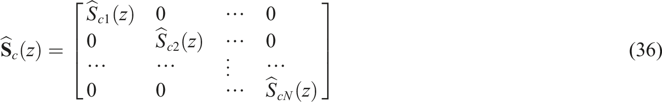
The coupling of the secondary channels is mathematically reflected in the non-diagonal elements of the secondary channel transfer function matrix. If we assume that the system is fully decoupled and neglect the non-diagonal elements, the secondary channel transfer function matrix can be simplified as a diagonal matrix, and the identification estimation model can be written as:

{\hat{S}}_{c} (z) = [\begin{array}{l} {\hat{S}}_{c 1} (z) & 0 & \dots & 0 \\ 0 & {\hat{S}}_{c 2} (z) & \dots & 0 \\ \dots & \dots & ⋮ & \dots \\ 0 & 0 & \dots & {\hat{S}}_{c N} (z) \end{array}]

(36)

The error signal in component form is given by:

e_{k} (n) = d_{k} (n) + S_{k k} (n) y_{k} (n) k = 1, 2, . . . N

(37)

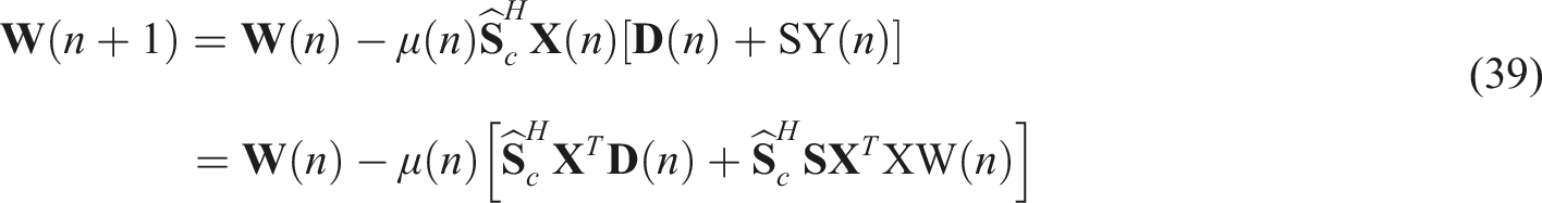
At this stage, the formula for updating the control weight coefficients is:

w_{k} (n + 1) = w_{k} (n) - μ_{k} (n) {\hat{S}}_{c k}^{H} (n) e_{k} (n) k = 1, 2, . . . N

(38)

However, in practical control systems, the error signal is still the collective result of all secondary channels. Substituting equation (31) into equation (38), the result can be obtained:

\begin{array}{l} W (n + 1) = W (n) - μ (n) {\hat{S}}_{c}^{H} X (n) [D (n) + SY (n)] \\ = W (n) - μ (n) [{\hat{S}}_{c}^{H} X^{T} D (n) + {\hat{S}}_{c}^{H} S X^{T} XW (n)] \end{array}

(39)

Assuming that the algorithm converges, we can determine the optimal solution for the control weight coefficients when $n \to \infty$ is set to a certain value.

W (\infty) = - {[{\hat{S}}_{c}^{H} S X^{T} X]}^{- 1} {\hat{S}}_{c}^{H} X^{T} D (n)

(40)

Subtracting the optimal solution from both sides of equation (39), it can be obtained:

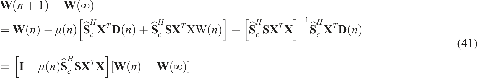
\begin{array}{l} W (n + 1) - W (\infty) \\ = W (n) - μ (n) [{\hat{S}}_{c}^{H} X^{T} D (n) + {\hat{S}}_{c}^{H} S X^{T} XW (n)] + {[{\hat{S}}_{c}^{H} S X^{T} X]}^{- 1} {\hat{S}}_{c}^{H} X^{T} D (n) \\ = [I - μ (n) {\hat{S}}_{c}^{H} S X^{T} X] [W (n) - W (\infty)] \end{array}

(41)

From equation (41), it can be seen that the control weight coefficients will converge as long as the modulus of the eigenvalue of $[I + μ (n) {\hat{S}}_{c}^{H} S X^{T} X]$ is less than 1.³¹ To ensure algorithm convergence for given secondary channels and reference input signals, the convergence can be guaranteed by adjusting the iteration step size. However, a step size that is too small may reduce the convergence speed. Furthermore, the convergence characteristics can be improved by adjusting the internal parameters of ${\hat{S}}_{c}$ . By comparing equations (34) and (39), we observe that the convergence of the original algorithm is related to ${\hat{S}}^{H} S$ under certain conditions of iteration step size and input signals, while the convergence of the decoupling algorithm is related to ${\hat{S}}_{c}^{H} S$ . Assuming accurate identification of the secondary channels, the algorithm will converge when the eigenvalue ${\hat{S}}^{H} S$ is a positive real number. In the decentralized decoupling algorithm, neglecting the non-diagonal elements of the matrix may lead to negative eigenvalues of the matrix ${\hat{S}}_{c}^{H} S$ , which could cause control divergence. To reduce the impact of ignoring the non-diagonal elements, the coupling effect between the secondary channels is fed back and compensated into their respective control loops. The k th main diagonal element of the matrix ${\hat{S}}_{c}$ in the time domain is expressed as:

{\hat{S}}_{c k} (n) = {\hat{S}}_{k k} (n) + \sum_{\begin{array}{l} i = 1 \\ i \neq k \end{array}}^{N} β_{k i} {\hat{S}}_{k i} (n)

(42)

where

β_{k i}

denotes the coupling feedback compensation factor, and the “amplitude weighting” method is used. The main channel has a weighting factor of 1, and the remaining channels are amplitude-weighted, which can be calculated using the following formula:

β_{k i} = | S_{k i} (n) | / \sum_{\begin{array}{l} i = 1 \\ i \neq k \end{array}}^{N} | S_{k i} (n) |

(43)

By compensating the coupling between channels in the form of weighted coefficients and feeding it back into their respective control loops, the identification accuracy is improved compared to simply ignoring the non-diagonal elements, and the distribution characteristics of the eigenvalue ${\hat{S}}_{c}^{H} S$ are also improved. By substituting equations (42) and (43) into equation (38), the control weight coefficient update criterion is obtained as follows:

w_{k} (n + 1) = w_{k} (n) - μ_{k} (n) {[{\hat{S}}_{k k} (n) + \sum_{\begin{array}{l} i = 1 \\ i \neq k \end{array}}^{N} (| S_{k i} (n) | / \sum_{\begin{array}{l} i = 1 \\ i \neq k \end{array}}^{N} | S_{k i} (n) |) {\hat{S}}_{k i} (n)]}^{H} e_{k} (n)

(44)

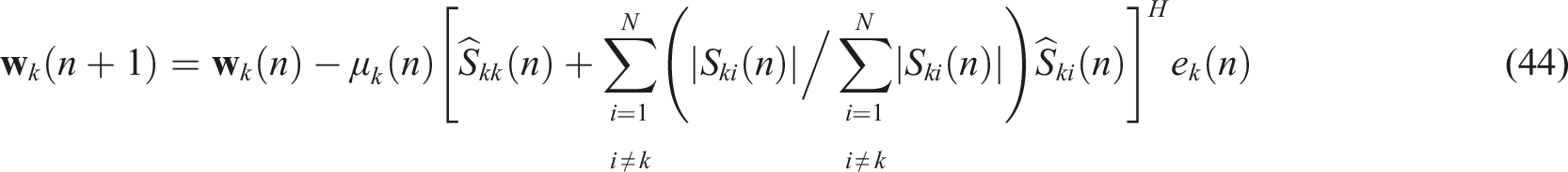
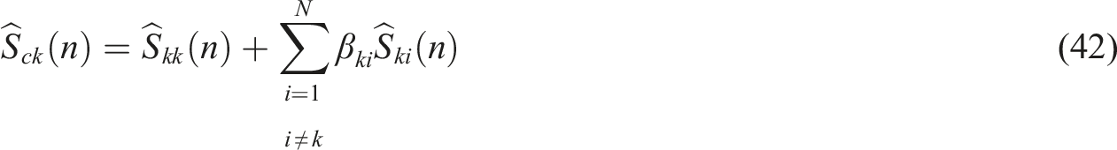
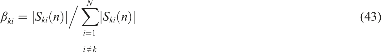
Equation (44) represents the control weight coefficient update formula for the multi-channel decentralized decoupling filtered-x least mean square algorithm (DMFxLMS). In the decoupling algorithm, each controller update is only related to the adjacent error signal, which greatly reduces the complexity of the computation. The control system is simplified to parallel single-channel loops, as shown in the algorithm structure in Figure 6.

Figure 6.

The algorithm structure of the multi-channel decentralized decoupling optimization.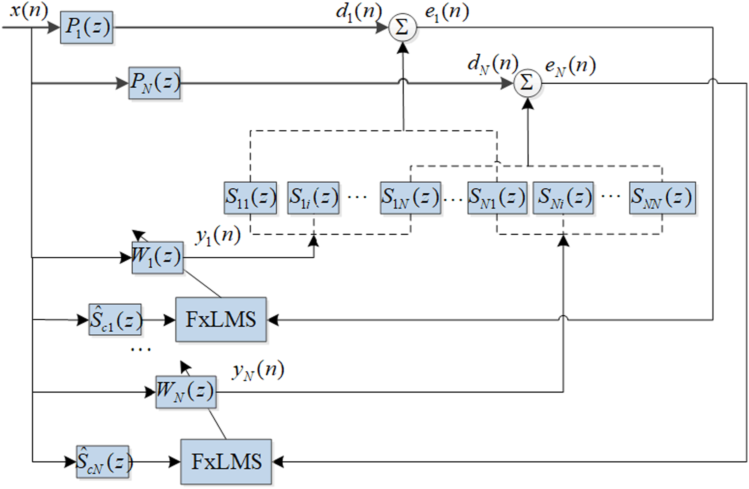

Design of anti-impact link

In the control process, when the system is subjected to shocks, the controller output tends to be large, which can easily enter the actuator saturation working zone, leading to unstable output force and adverse effects on control performance and stability. The effect of shocks on control stability is shown in Figure 7. To improve the robustness of the control algorithm, the algorithm can be improved in the two stages of the error signal entering the controller and the control output signal entering the actuator.

Figure 7.

The effect of shocks on control system.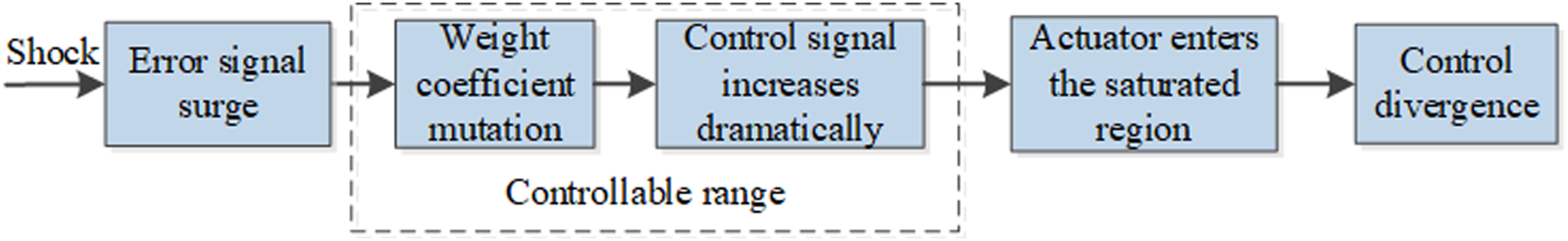

Impact mitigation factor

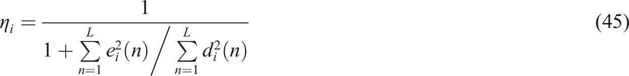
In the DMFxLMS algorithm, the coefficients’ control authority remains constant during the data input phase, with the error signal regulating the coefficients. To address this, an impact mitigation factor, designated as $η_{i}$ is introduced into the coefficient update, where i represents the channel number. $η_{i}$ is based on the ratio of the energy of the error signal within a data block to the expected signal energy that is basic design, and it can be expressed as:

η_{i} = \frac{1}{1 + \sum_{n = 1}^{L} e_{i}^{2} (n) / \sum_{n = 1}^{L} d_{i}^{2} (n)}

(45)

where L represents the length of the data block,

d_{i} (n)

e_{i} (n)

refers to the expected signal and error signal within the data block,

d_{i} (n) = P_{i} (z) x (n)

and

e_{i} (n)

are directly obtained from the error sensors. The revised coefficient update equation is as follows:

W_{i H}^{q} (k + 1) = W_{i H}^{q} (k) - η_{i} \frac{u_{i}^{q} (k)}{L} FHT [\begin{array}{l} Δ W_{i H}^{q} (k) \\ 0 \end{array}]

(46)

where FHT refers to fast Hartley transform.³² From equation (45), it can be observed that in a stable control state, the

d_{i}^{2} (n) ≫ e_{i}^{2} (n)

and

η_{i} \to 1

coefficient update equations remain relatively unchanged. When the base experiences an impact from other mechanical devices,

d_{i}^{2} (n) ≪ e_{i}^{2} (n)

and

0 < η_{i} ≪ 1

, the weight correction term toward zero, and the control coefficients remain constant. The incorporation of the impact mitigation factor effectively addresses the issue of sudden changes in the control coefficients due to abrupt fluctuations in the error signal.

Output saturation mitigation

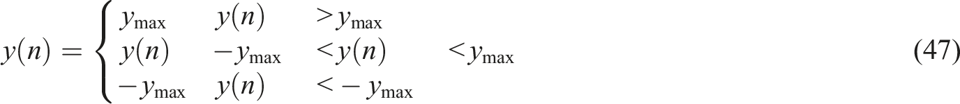
In the block algorithm, the control signals are still outputted in point form to the amplifier which drives the actuator. It is necessary to suppress the saturation of the output control signals. For an ideal saturation function, a threshold $y_{\max}$ can be directly specified. If the output signal exceeds the threshold, it will be clamped; otherwise, the output signal will be output as is, which can be represented by a piecewise function:

y (n) = {\begin{cases} y_{\max} & y (n) & > y_{\max} \\ y (n) & - y_{\max} & < y (n) & < y_{\max} \\ - y_{\max} & y (n) & < - y_{\max} \end{cases}

(47)

For rotating machinery-induced spectral vibrations, the output control signals are usually sinusoidal in nature. Directly limiting the output signals using a piecewise function form amounts to clipping the sinusoidal signal, which is detrimental to control stability. The output signal suppression process should be gradual and smooth. For output control signals that approach or exceed the saturation output, a percentage limit is imposed, such that the changing trend is as close as possible to the original state. The percentage function can be represented as:

f (y) = \frac{a}{b y^{2} + 1}

(48)

where a is the proportional coefficient and b is the amplitude adjustment coefficient and is related to the extent of control signal overflow. The overall requirement for the function

f (y)

is that when the output signal is below the saturation value

f (y) \to 1

, and when it approaches or exceeds saturation,

f (y) \to κ

and

κ

are derivative of the overflow coefficient. In practical control systems, the saturation threshold can be pre-determined based on the requirements for actuator usage, which in turn determines the range of values for the proportional coefficient and adjustment coefficient.

Suppose the maximum working current of the actuator is 10A and the power amplifier used in the system is a 1:1 amplifier, then the controller’s output analog signal will not exceed 10. If the output signal caused by shock vibrations is set to be the superposition of four spectra with amplitudes of 10 and different frequencies, then the proportional coefficient a is set to 0.9 and the amplitude adjustment coefficient b is set to 0.002 based on the calculation. The percentage function and the output signals before and after saturation suppression are shown in Figure 8, respectively.

Figure 8.

Percentage function and its suppression effect on output signals. (a) Percentage function. (b) Comparison of output before and after saturation function suppression.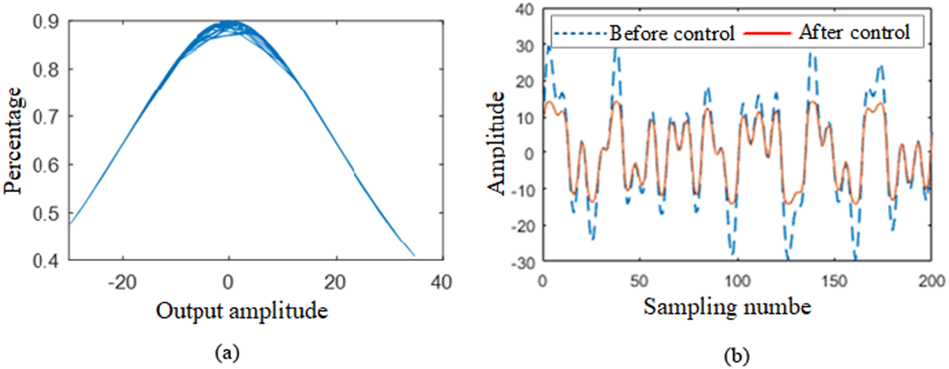

As seen in the figure, the percentage function decreases as the magnitude of the output signal increases. When the output signal’s magnitude is less than the pre-determined threshold, the suppressed signal can approximate the original output signal with high accuracy. However, once the output signal approaches or exceeds the pre-determined threshold, the suppressed output signal stabilizes around 10A, following the original signal’s trend, in a gradual and steady manner. Through simulation analysis, it was found that when the control output signal was greatly exceeded by the impact response, no matter how the proportion coefficient and amplitude adjustment coefficient were adjusted, the approximation accuracy at low magnitudes and the suppression effect at high magnitudes were contradictory. To balance both, the percentage function was set as a piecewise function:

{\begin{cases} f (y) = a_{1} / (b y^{2} + 1) | y | < y_{\max} \\ f (y) = a_{2} / (b y^{2} + 1) | y | > y_{\max} \end{cases}

(49)

Figure 9 illustrates the improved percentage function and its ability to suppress overflow control signals. The improved percentage function has stronger suppression capabilities while still maintaining accuracy in lower amplitude outputs and maintaining a steady and gradual output signal.

Figure 9.

Improved percentage function and its effect on output signal suppression. (a) Percentage function. (b) Comparison of output before and after saturation function suppression.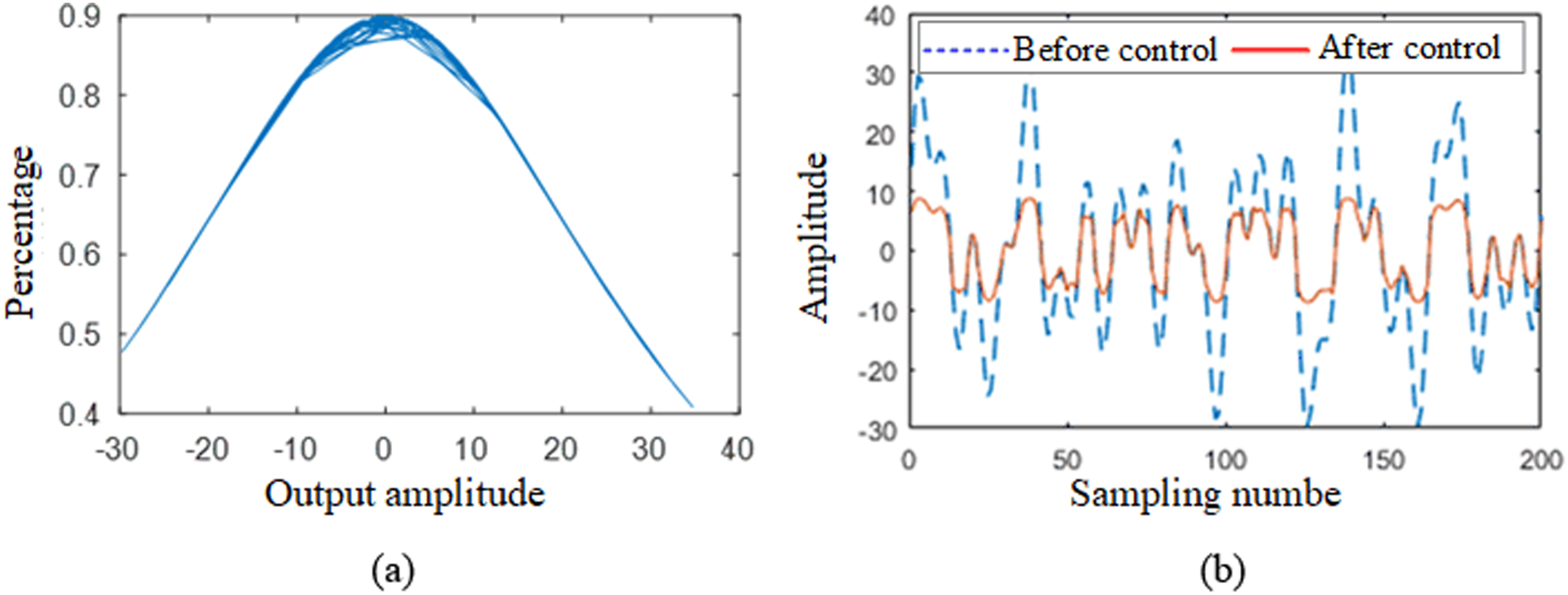

Simulation analysis

To assess the performance of the DMFxLMS algorithm, a four-channel control model was constructed using MATLAB/Simulink. Active control simulation analyses were carried out employing both the MFxLMS and DMFxLMS algorithms. The control filter featured an order of 256, a data block length of 256, and a sampling frequency of 1 kHz. The excitation signals were configured as fixed-frequency sinusoidal signals superimposed at 30 Hz, 37 Hz, 60 Hz, and 110 Hz, and sinusoidal sweep frequency signals superimposed at 28–31 Hz, 35–38 Hz, 58–61 Hz, and 108–111 Hz. Moreover, a 30 dB signal-to-noise ratio white noise was added to each signal.

By applying the MFxLMS algorithm for the four-channel control simulation, the iteration step size was designated as $5 \times 10^{- 5}$ . The error signal time history at the four measurement points is depicted in Figures 10 and 11.

Figure 10.

Control effect of MFxLMS algorithm under fixed-frequency excitation. (a) Time history diagram of error signal at measurement point 1#. (b) Time history diagram of error signal at measurement point 2#. (c) Time history diagram of error signal at measurement point 3#. (d) Time history diagram of error signal at measurement point 4#.

Figure 11.

Control effect of MFxLMS algorithm under sweep frequency excitation. (a) Time history diagram of error signal at measurement point 1#. (b) Time history diagram of error signal at measurement point 2#. (c) Time history diagram of error signal at measurement point 3#. (d) Time history diagram of error signal at measurement point 4#.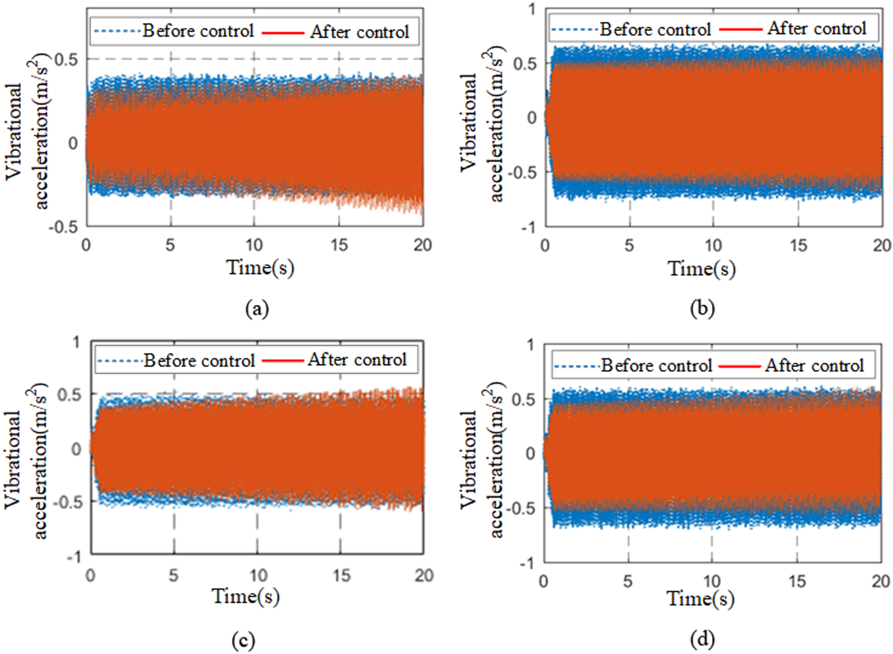

As can be seen from Figures 10 and 11, the MFxLMS algorithm does not exhibit significant control effects for either fixed-frequency or fluctuating line spectrum excitations, and even demonstrates instances of control instability.

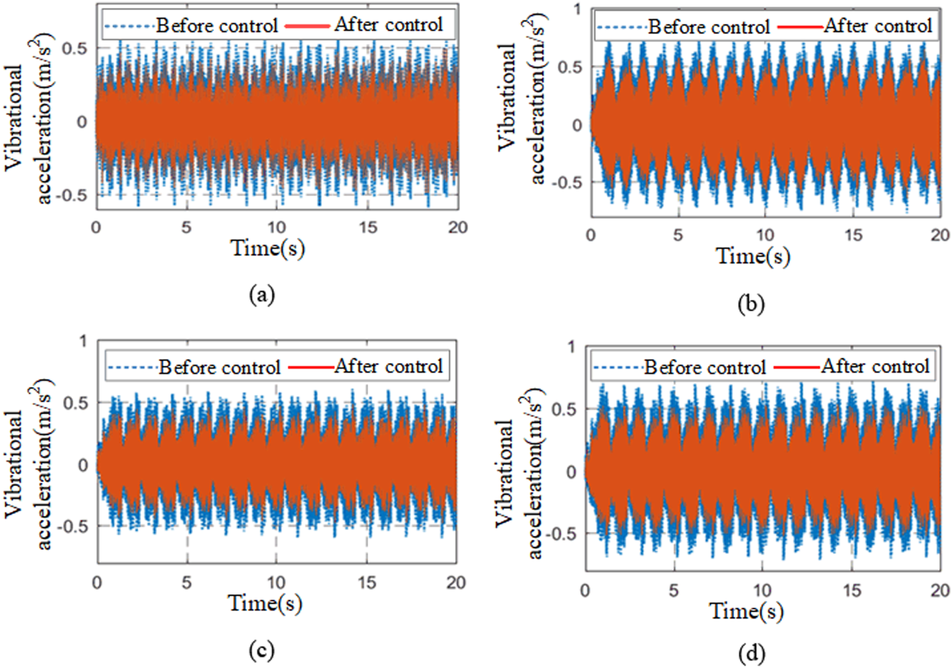
By employing the DMFxLMS algorithm for simulation analysis, the time history of error signals at the four measurement points before and after control under different excitations is shown in Figure 12 and Figure 13.

Figure 12.

Control effect of DMFxLMS algorithm under fixed-frequency excitation. (a) Time history diagram of error signal at measurement point 1#. (b) Time history diagram of error signal at measurement point 2#. (c) Time history diagram of error signal at measurement point 3#. (d) Time history diagram of error signal at measurement point 3#.

Figure 13.

Control effect of DMFxLMS algorithm under fixed-frequency excitation. (a) Time history diagram of error signal at measurement point 1#. (b) Time history diagram of error signal at measurement point 2#. (e) Time history diagram of error signal at measurement point 3#. (f) Time history diagram of error signal at measurement point 4#.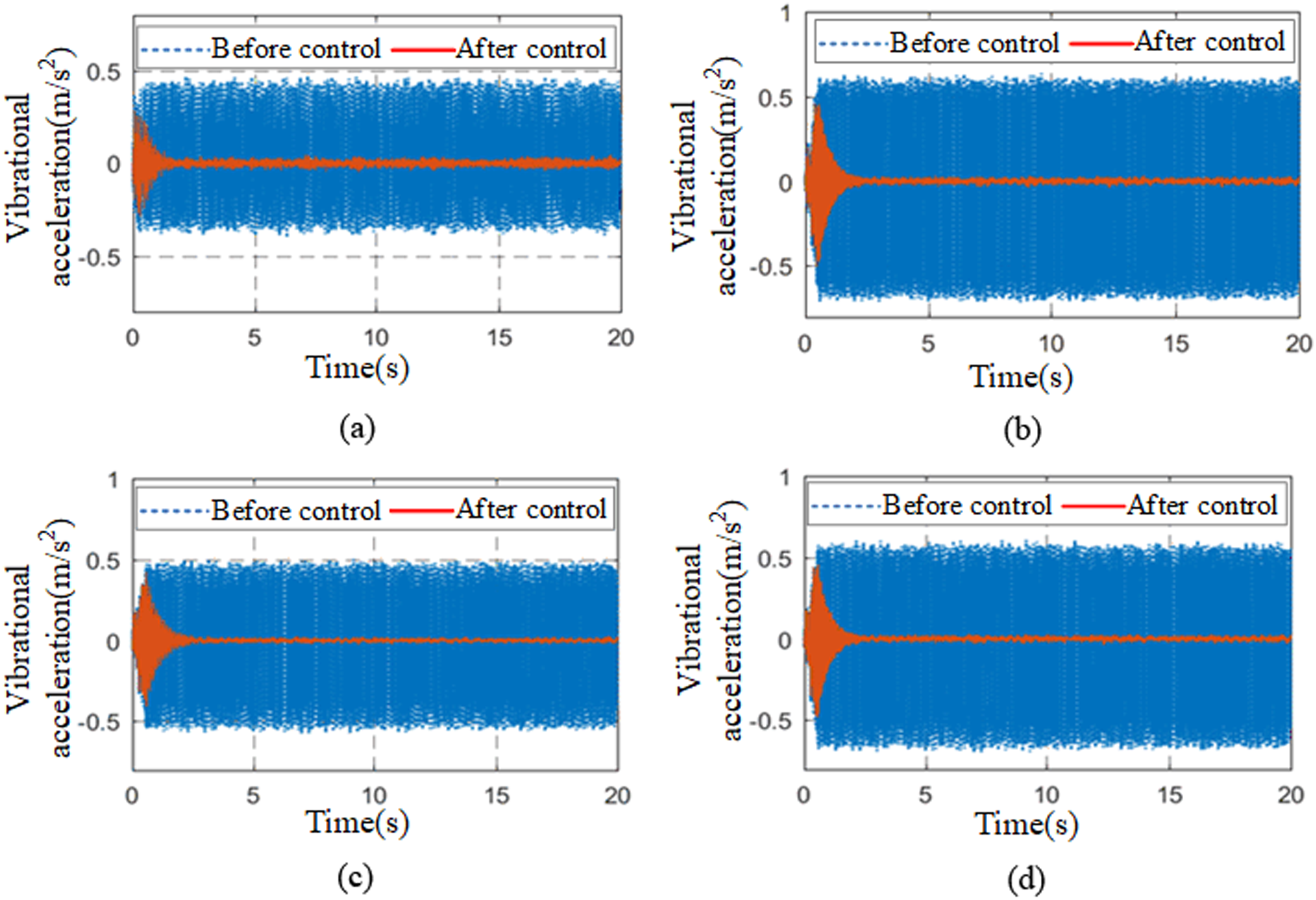

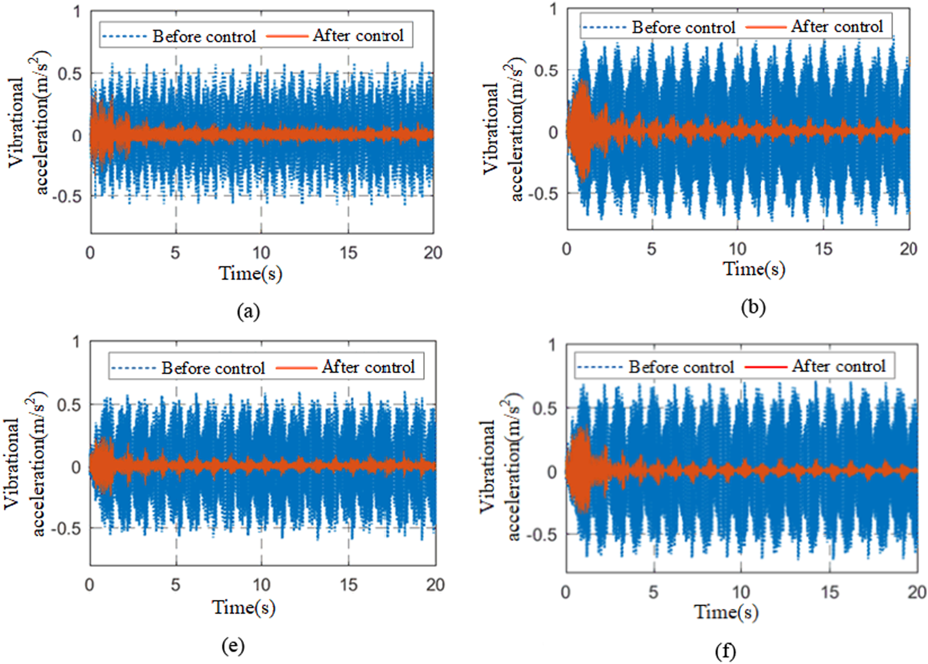
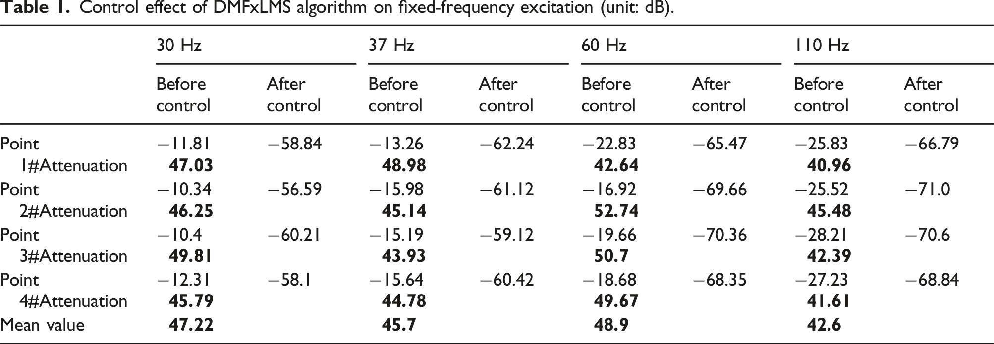
A comparison of the control effects of the two algorithms under the same excitation reveals that the DMFxLMS algorithm demonstrates remarkable control performance, with specific control results shown in Tables 1 and 2.

Table 1.

Control effect of DMFxLMS algorithm on fixed-frequency excitation (unit: dB).

	30 Hz		37 Hz		60 Hz		110 Hz
	Before control	After control	Before control	After control	Before control	After control	Before control	After control
Point 1#Attenuation	−11.81	−58.84	−13.26	−62.24	−22.83	−65.47	−25.83	−66.79
Point 1#Attenuation	47.03		48.98		42.64		40.96
Point 2#Attenuation	−10.34	−56.59	−15.98	−61.12	−16.92	−69.66	−25.52	−71.0
Point 2#Attenuation	46.25		45.14		52.74		45.48
Point 3#Attenuation	−10.4	−60.21	−15.19	−59.12	−19.66	−70.36	−28.21	−70.6
Point 3#Attenuation	49.81		43.93		50.7		42.39
Point 4#Attenuation	−12.31	−58.1	−15.64	−60.42	−18.68	−68.35	−27.23	−68.84
Point 4#Attenuation	45.79		44.78		49.67		41.61
Mean value	47.22		45.7		48.9		42.6

Table 2.

Control effect of DMFxLMS algorithm on sweep frequency excitation (unit: dB).

	28–31 Hz		35–38 Hz		58–61 Hz		108–111 Hz
	Before control	After control	Before control	After control	Before control	After control	Before control	After control
Point 1#Attenuation	−14.44	−45.73	−13.6	−41.93	−21.45	−39.71	−29.79	−58.1
Point 1#Attenuation	31.29		28.33		18.26		28.31
Point 2#Attenuation	−13.32	−38.73	−21.58	−47.11	−18.67	−44.63	−29.7	−50.91
Point 2#Attenuation	25.41		25.53		25.96		21.21
Point 3#Attenuation	−14.78	−42.07	−17.42	−42.23	−29.01	−49.64	−35.73	−59.7
Point 3#Attenuation	27.29		24.81		20.63		23.97
Point 4#Attenuation	−14.76	−41.5	−16.15	−44.53	−22.89	−50.16	−31.47	−58.7
Point 4#Attenuation	26.74		28.38		27.27		27.23
Mean value	27.69		26.76		24.03		25.18

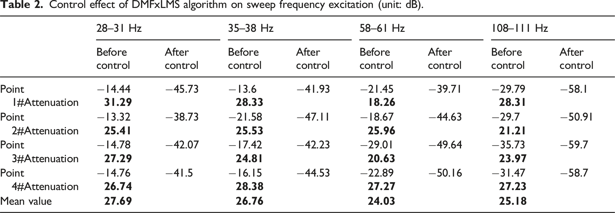
Based on the analysis presented above, it can be inferred that.

(1) When employing the MFxLMS algorithm directly for control, the four measurement points mutually constrain and influence each other, resulting in a slower convergence rate. Moreover, the algorithm is incapable of simultaneously controlling multiple line spectra, leading to an unstable control process. During the later stages of control, the error signal worsens, suggesting that the MFxLMS algorithm’s effectiveness in controlling four-channel multi-frequency excitations is suboptimal.

(2) The DMFxLMS algorithm is capable of effectively controlling multiple line spectra concurrently while exhibiting rapid convergence properties, reducing the convergence time to 2–3 s. It demonstrates commendable control performance at all four measurement points. The average power spectral attenuation for the fixed-frequency line spectra at 30 Hz, 37 Hz, 60 Hz, and 110 Hz is 47.22 dB, 45.7 dB, 48.9 dB, and 42.6 dB, respectively. Meanwhile, the average power spectral attenuation for the sweep frequency bands of 28–31 Hz, 35–38 Hz, 58–61 Hz, and 108–111 Hz is 27.69 dB, 26.76 dB, 24.03 dB, and 25.18 dB, respectively.

Experimental research

Utilizing a hybrid active-passive isolator as the actuating structure and the high real-time performance and powerful computational capabilities of the NI-PXIe measurement and control hardware, a two-layer isolation experimental system is constructed. Control algorithm programs are developed using LabVIEW to conduct channel identification and active isolation control experiments, offering experimental support for verifying the effectiveness of the DMFxLMS algorithm.

Development of the NI-PXIe control system and isolation test bed

The two-layer isolation test bed is depicted in Figure 14. An exciter is mounted as the vibration source on the upper layer of the test bed, while a mass block is added as a counterweight to enhance the total supported weight of the isolator. The acceleration signal generated by the vibration source serves as the reference signal for the entire system. Integrated active-passive isolators are positioned at the four corners of the middle layer, functioning as secondary vibration sources. They are connected to the upper and lower frames using bolts, with acceleration sensors installed close to the upper and lower connection points. The sensors on the upper layer act as monitoring signals, while those on the lower layer serve as error signals. The isolation effect can be directly observed through the acceleration signals from the upper and lower layers. The middle layer is connected to the base via elastic supports, and its dynamic characteristics can be simplified to a spring-damper structure.

Figure 14.

Two-layer isolation test bed. (a) Schematic diagram. (b) Physical diagram.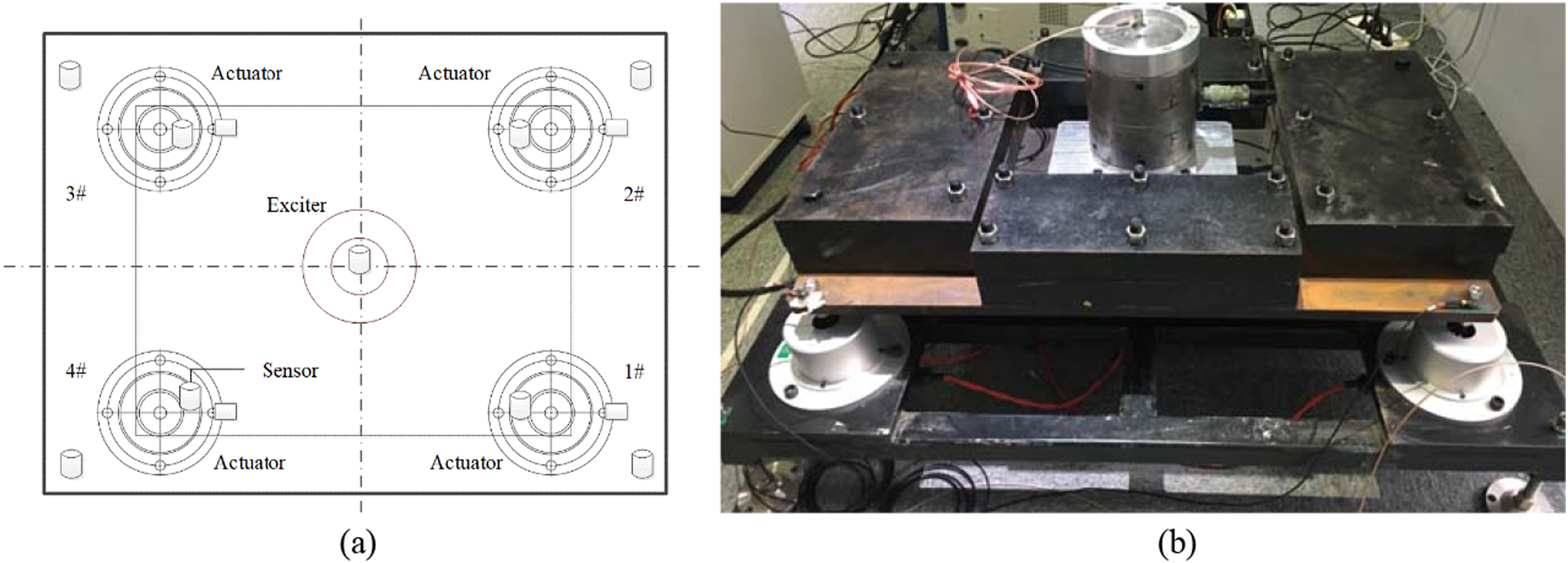

The primary parameters of the isolation test bed include: exciter with 220V voltage, a maximum output force of 1000N, and a weight of 40 kg; upper layer frame with a self-weight of 120 kg, counterweight mass block, and a total weight of 380 kg; four electromagnetic rubber hydraulic integrated isolators with 220V voltage and an individual weight of 10.8 kg; middle layer frame with a mass of 40 kg.

Figure 15 presents a signal flow chart of the four-channel control system. The signal acquisition process is indicated by the blue lines, while the signal output process is represented by the red lines. The acceleration sensor captures reference signals and error signals, which are then transmitted to the RT (real-time) controller through the input board card. The control algorithm is applied to obtain four control signals, which are then transmitted to the power amplifier via the output board card. This drives the integrated vibration isolation device to produce control force and reduces vibration transmission to the base, enabling active control testing. At the same time, another NI-PXIe driver is used to excite the upper layer exciter, and all acceleration signals from both the upper layer stand and intermediate layer stand are collected for real-time monitoring and subsequent data processing.

Figure 15.

Four-channel control system signal flow chart.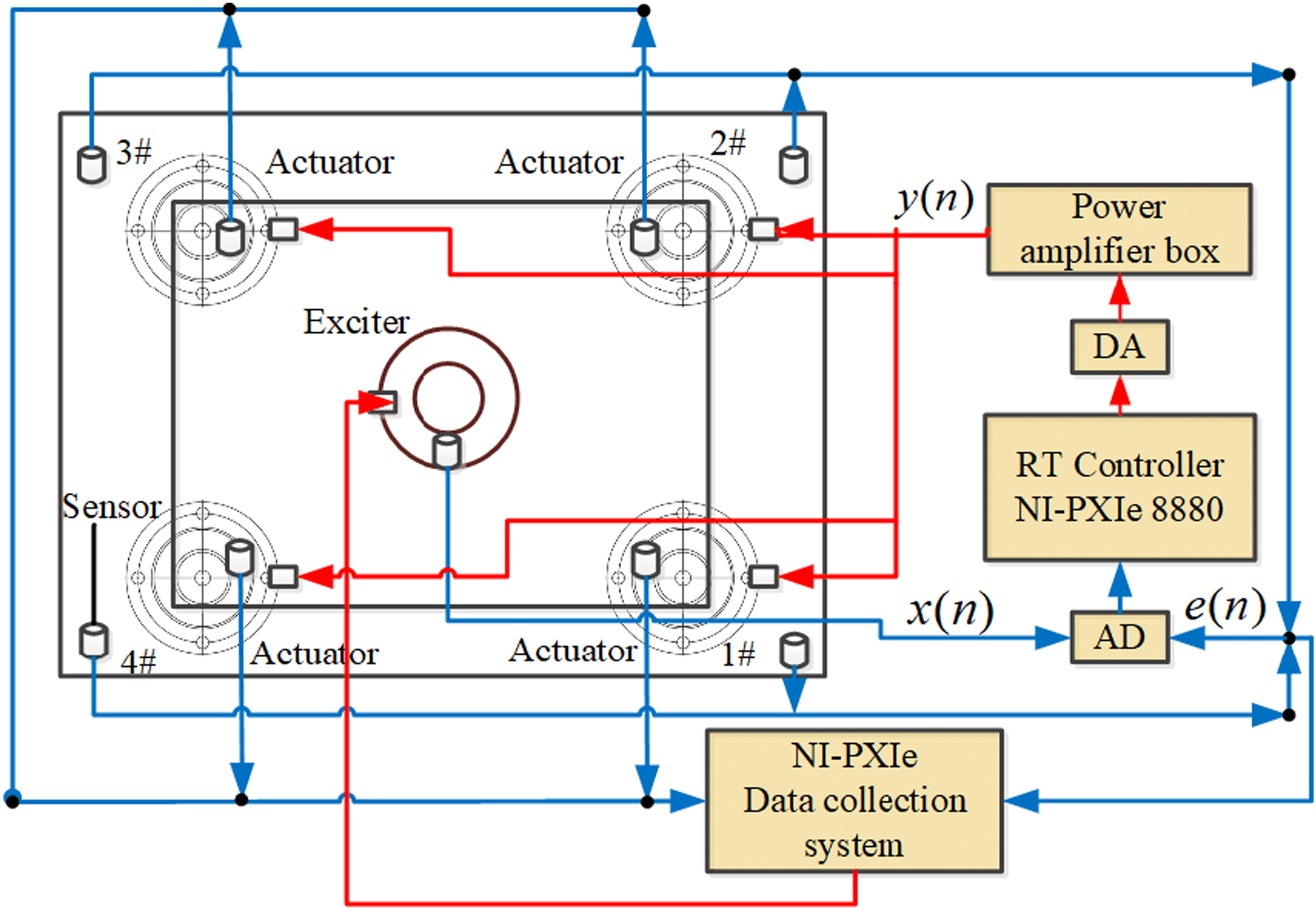

Offline identification of primary and secondary channels

This study employed a passive-active hybrid vibration isolator with stable output performance, and the secondary channel characteristics remain largely unchanged during the control process. The recursive least squares (RLS) identification algorithm, equipped with a forgetting factor, is utilized to perform offline identification of 16 secondary channels and 4 primary channels. The lower computer generates white noise in the frequency range of 1–200 Hz, which is filtered and then converted from digital to analog (DA) and output to four actuators, with a current of 3A. The identification filter has a length of 150 orders, a forgetting factor of $γ = 0.98$ , a sampling frequency of 1 KHz, and an identification time of 10s. The white noise signal and error signals from four measurement points are collected as the input and ideal output of the identification filter, respectively, and the identification algorithm is used to obtain the coefficients of the identification filter. Diagram 5.3 displays the results of the identification of the 16 secondary channels, where $S_{i j}$ represents the secondary channel between the error signal of the ith actuator and the jth measurement point Figure 16.

Figure 16.

Secondary channel identification estimation model. (a) No. 1 Actuator to No. 1 Error Signal - S11. (b) No. 1 Actuator to No. 2 Error Signal - S12. (c) No. 1 Actuator to No. 3 Error Signal - S13. (d) No. 1 Actuator to No. 1 Error Signal - S14. (e) No. 2 Actuator to No. 1 Error Signal - S21. (f) No. 2 Actuator to No. 2 Error Signal - S22. (g) No. 2 Actuator to No. 3 Error Signal - S23. (h) No. 2 Actuator to No. 4 Error Signal - S24. (i) No. 3 Actuator to No. 1 Error Signal - S31. (j) No. 3 Actuator to No. 2 Error Signal - S32. (k) No. 3 Actuator to No. 3 Error Signal - S33. (l) No. 1 Actuator to No. 4 Error Signal - S34. (m) No. 4 Actuator to 1st Error Signal - S41. (n) No. 4 Actuator to No. 2 Error Signal - S42. (o) No. 4 Actuator to No. 3 Error Signal - S43. (p) No. 4 Actuator to No. 4 Error Signal - S44.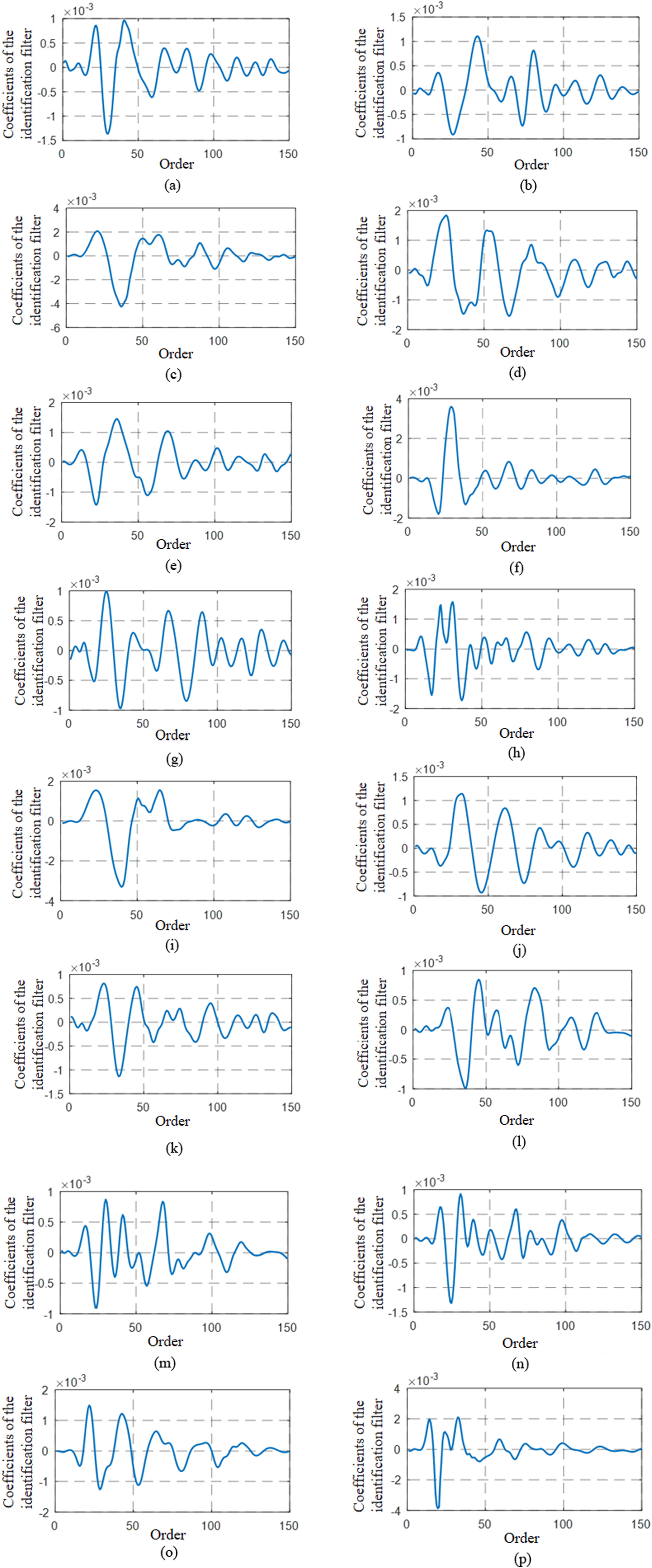

The primary channel identification was performed using the same identification algorithm with a 128th order and utilizing 1–200 Hz white noise excitation on the upper layer exciter, collecting the error signals at four measurement points as the target signal for channel identification. The results are shown in Figure 17, where $P_{i} (i = 1, 2, 3, 4)$ represents the estimated model of the four primary channels, respectively.

Figure 17.

Primary channel identification estimation model. (a) 1# Primary channel. (b) 2# Primary channel. (c) 3# Primary channel. (d) 4# Primary channel.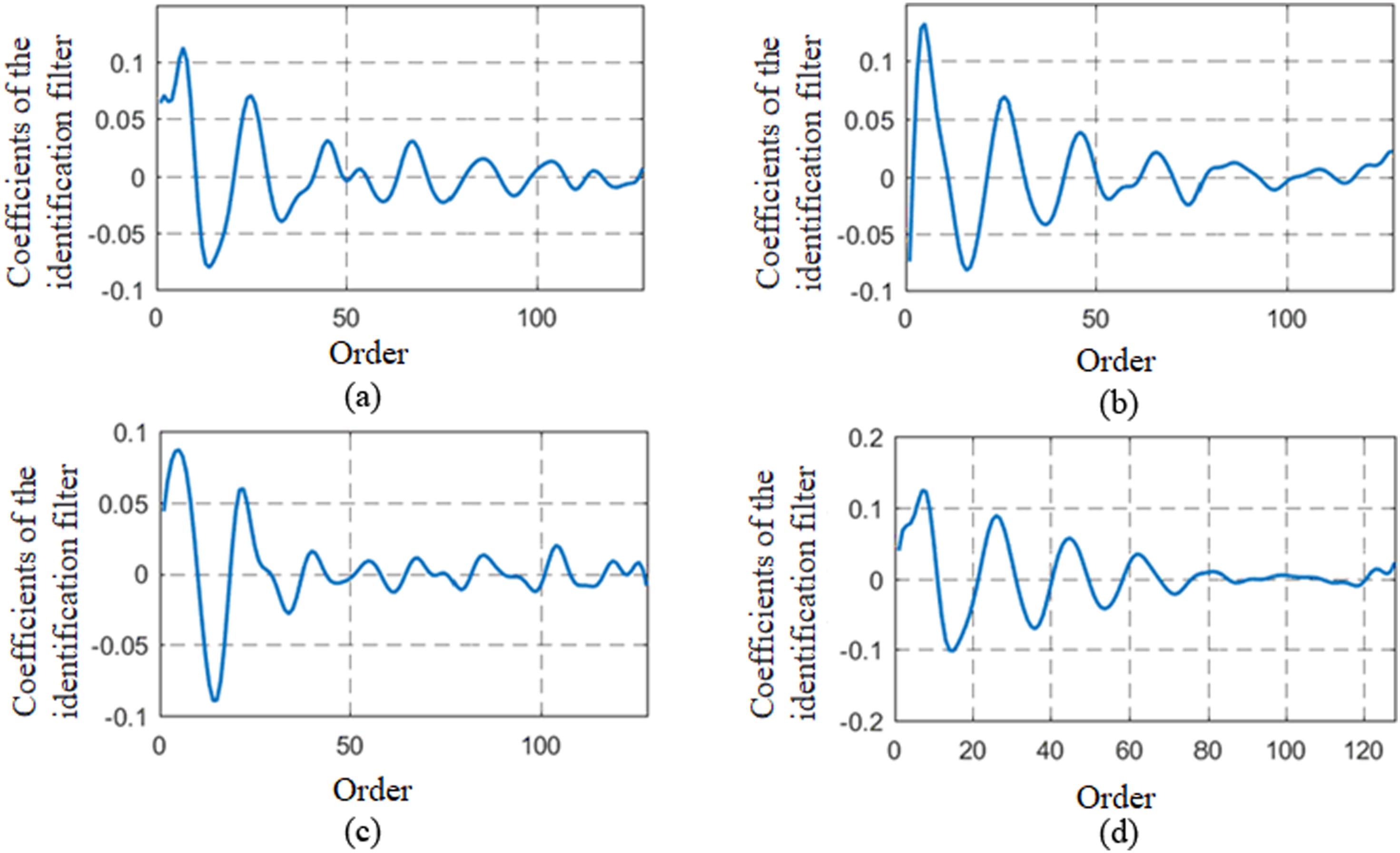

Isolation control experiment and analysis

In order to perform an active control experiment, incorporate the estimated secondary channel into the control system. To closely approximate the frequency spectrum components under the operating conditions of a ship-borne diesel engine, the excitation signal of the exciter is set to a sinusoidal waveform with frequencies of 30 Hz, 37 Hz, 60 Hz, and 110 Hz, along with partial harmonic spectra and white noise with an amplitude of 0.1 A and a frequency range of 30–60 Hz. The sample rate is set to 1 KHz, and the four-channel output voltages have an amplitude of $| y | < 9 A$ . The control system has 256 stages, and all collected signals are filtered through a 200 Hz low-pass filter using a 3rd-order Butterworth filter. The specific steps of the experiment are as follows:

(1) Output the excitation signal through the PXI-6733 to the amplifier, which drives the exciter to produce a reference signal. After the vibration stabilizes, start the data acquisition system and collect the upper layer signal and error signal to evaluate the passive isolation effect.

(2) Set the initial iteration step size for each control loop (corrected according to empirical formula, the iterative step length of the algorithm is adjusted to its optimal value), activate the control, and wait for the error signal to converge and stabilize before disabling the control system and data acquisition system.

(3) Process the collected signals by plotting the upper layer signal and error signal corresponding to each measurement point on the same time history graph in the time domain. The graph represents the passive isolation effect before control, the convergence performance, control accuracy, etc. after control. Power spectrum analysis is performed on 10,000 points of the error signal before and after control, and the power spectrum decay of the error signal before and after control is used as the evaluation index for isolation.

Fixed-frequency spectrum excitation active control experiment

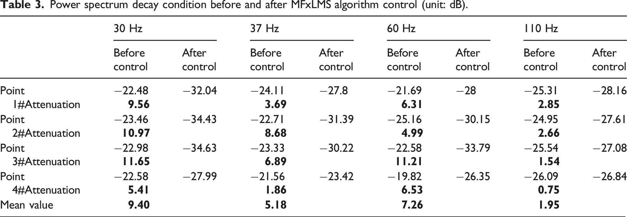
Figure 18 displays the time history graphs and power spectrums before and after control for the error signals of four measurement points. After collecting data for 18 s, the active control was initiated. The red line in the time domain graph represents the error signal, while the blue line represents the corresponding upper layer signal. After control was initiated, the amplitude of the error signal decreased at a slow pace, with the maximum reduction being less than 25%. There was essentially no control effect observed. Table 3 lists the specific control effect for each of the four measurement points.

Figure 18.

Control effect of MFxLMS algorithm. (a) Time history diagram of error signal at measurement point 1#. (b) Power spectrum of error signal at measurement point 1#. (c) Time history diagram of error signal at measurement point 2#. (d) Power spectrum of error signal at measurement point 2#. (e) Time history diagram of error signal at measurement point 3#. (f) Power spectrum of error signal at measurement point 3#. (g) Time history diagram of error signal at measurement point 4#. (h) Power spectrum of error signal at measurement point 4#.

Table 3.

Power spectrum decay condition before and after MFxLMS algorithm control (unit: dB).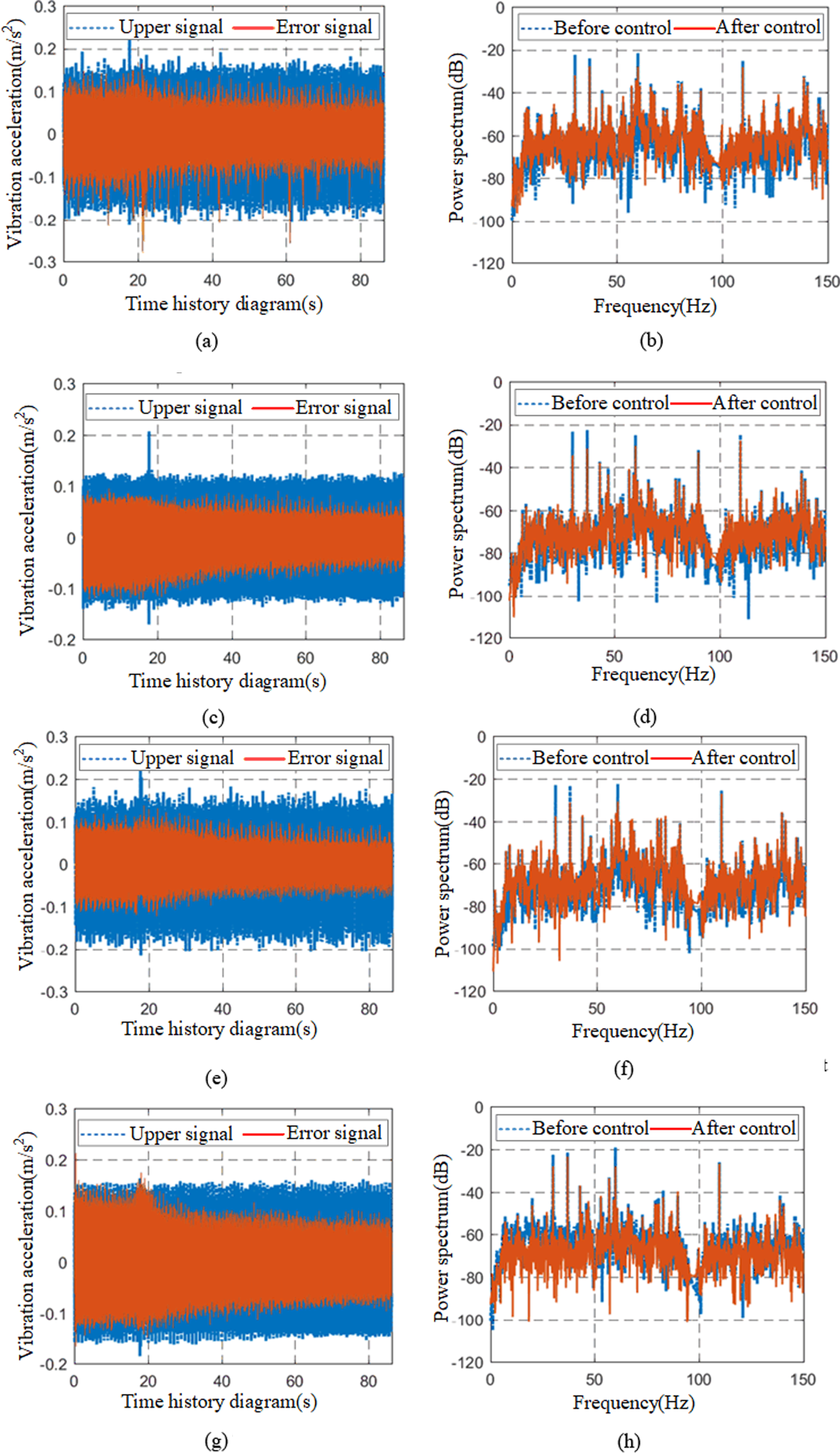

	30 Hz		37 Hz		60 Hz		110 Hz
	Before control	After control	Before control	After control	Before control	After control	Before control	After control
Point 1#Attenuation	−22.48	−32.04	−24.11	−27.8	−21.69	−28	−25.31	−28.16
Point 1#Attenuation	9.56		3.69		6.31		2.85
Point 2#Attenuation	−23.46	−34.43	−22.71	−31.39	−25.16	−30.15	−24.95	−27.61
Point 2#Attenuation	10.97		8.68		4.99		2.66
Point 3#Attenuation	−22.98	−34.63	−23.33	−30.22	−22.58	−33.79	−25.54	−27.08
Point 3#Attenuation	11.65		6.89		11.21		1.54
Point 4#Attenuation	−22.58	−27.99	−21.56	−23.42	−19.82	−26.35	−26.09	−26.84
Point 4#Attenuation	5.41		1.86		6.53		0.75
Mean value	9.40		5.18		7.26		1.95

Based on the results of the previous set of experiments, the influence of secondary channel coupling was taken into account and compensated within the respective control circuits for a vibration test.Figure 19 displays the temporal evolution of the error signals for each of the four measurement points, as well as the power spectrums before and after control. The active control was initiated at 23 s and completed at 25.5 s, resulting in a substantial improvement in the convergence speed. The amplitude of the error signal decreased by as much as 85%, and the spectra at the four measurement points were effectively suppressed, with the control-induced changes no longer being readily noticeable against the background noise. No other frequency oscillations were observed to be excited. The specific control performance is shown in Table 4.

Figure 19.

The control performance of the DMFxLMS algorithm. (a) Time history diagram of error signal at measurement point 1#. (b) Power spectrum of error signal at measurement point 1#. (c) Time history diagram of error signal at measurement point 2#. (d) Power spectrum of error signal at measurement point 2#. (e) Time history diagram of error signal at measurement point 3#. (f) Power spectrum of error signal at measurement point 3#. (g) Time history diagram of error signal at measurement point 4#. (h) Power spectrum of error signal at measurement point 4#.

Table 4.

Power spectrum decay condition before and after DMFxLMS algorithm control (unit: dB).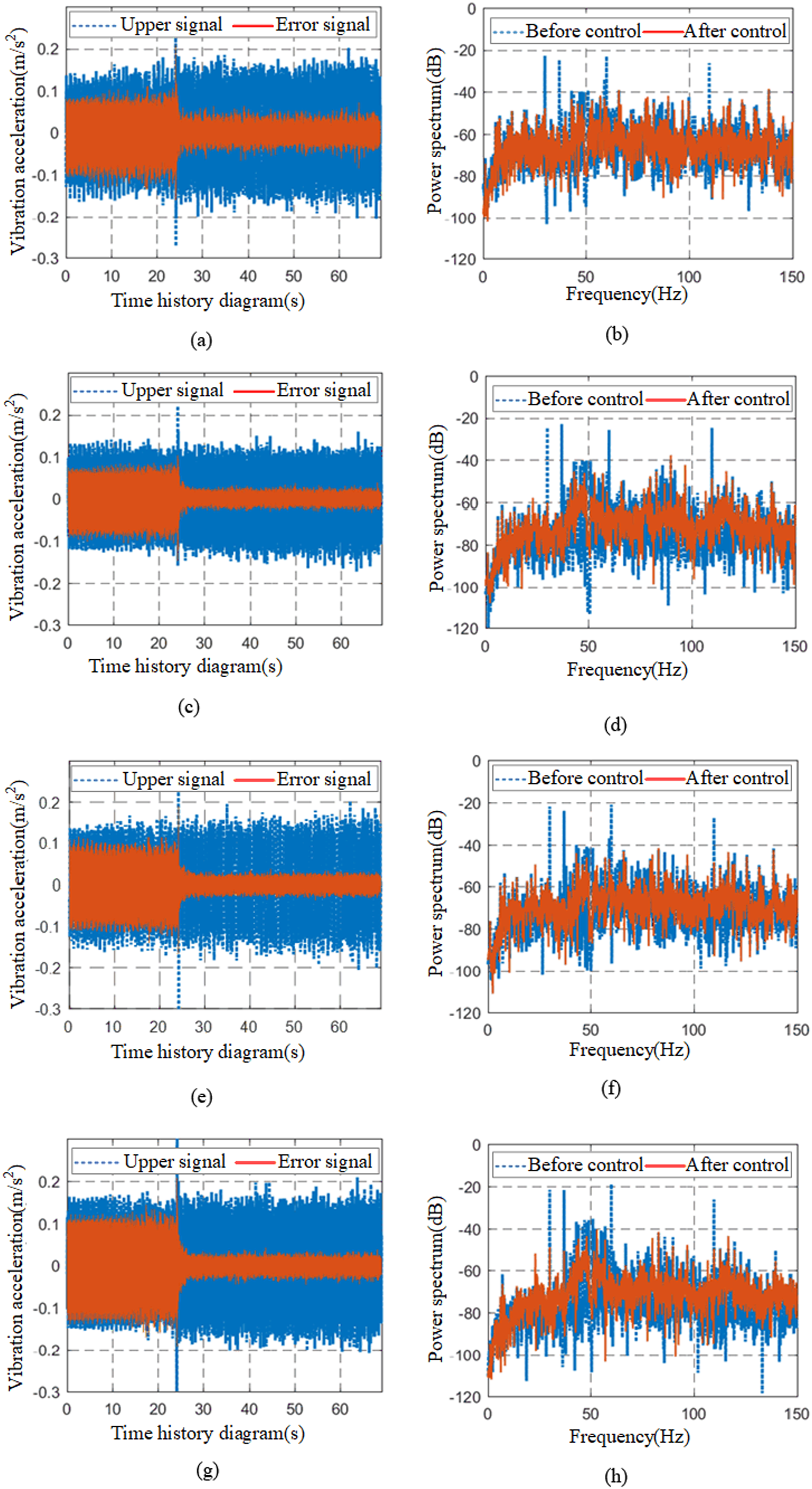

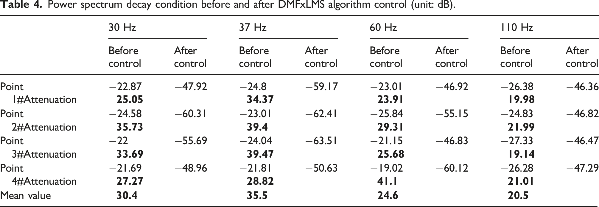
	30 Hz		37 Hz		60 Hz		110 Hz
	Before control	After control	Before control	After control	Before control	After control	Before control	After control
Point 1#Attenuation	−22.87	−47.92	−24.8	−59.17	−23.01	−46.92	−26.38	−46.36
Point 1#Attenuation	25.05		34.37		23.91		19.98
Point 2#Attenuation	−24.58	−60.31	−23.01	−62.41	−25.84	−55.15	−24.83	−46.82
Point 2#Attenuation	35.73		39.4		29.31		21.99
Point 3#Attenuation	−22	−55.69	−24.04	−63.51	−21.15	−46.83	−27.33	−46.47
Point 3#Attenuation	33.69		39.47		25.68		19.14
Point 4#Attenuation	−21.69	−48.96	−21.81	−50.63	−19.02	−60.12	−26.28	−47.29
Point 4#Attenuation	27.27		28.82		41.1		21.01
Mean value	30.4		35.5		24.6		20.5

Based on the analysis presented above, it can be inferred that.

(1) When the coupling between secondary channels was not taken into consideration, the algorithm had a very slow convergence speed and poor control performance, essentially operating in a state of control failure.

(2) Upon incorporating optimized control to disperse the coupling between the secondary channels, the entire control system was streamlined into a parallel single-channel control circuit. Significant control performance was observed at each of the four measurement points, with the convergence speed being significantly improved. The convergence control time was reduced to just 2.5 s. The average decline in power spectrums for the 30 Hz, 37 Hz, 60 Hz, and 110 Hz fixed-frequency spectra was 30.4 dB, 35.5 dB, 24.6 dB, and 20.5 dB, respectively.

Experiment on active control with fluctuating frequency spectral excitation

In the operation of marine diesel engines, the vibration frequency may experience severe fluctuations within a small range. Thus, it is crucial to examine the control algorithms under fluctuating frequency conditions. The reference signal is set to four chirp signals with a period of 1 s, each having a frequency change range of 28–31 Hz, 35–38 Hz, 58–61 Hz, and 108–111 Hz. Additionally, white noise with amplitude 0.1 A in the frequency range of 30–60 Hz is added. The control parameters are consistent with the constant frequency excitation control experiment, and the evaluation criterion for vibration isolation performance remains the reduction of the power spectrum of the error signal before and after control.

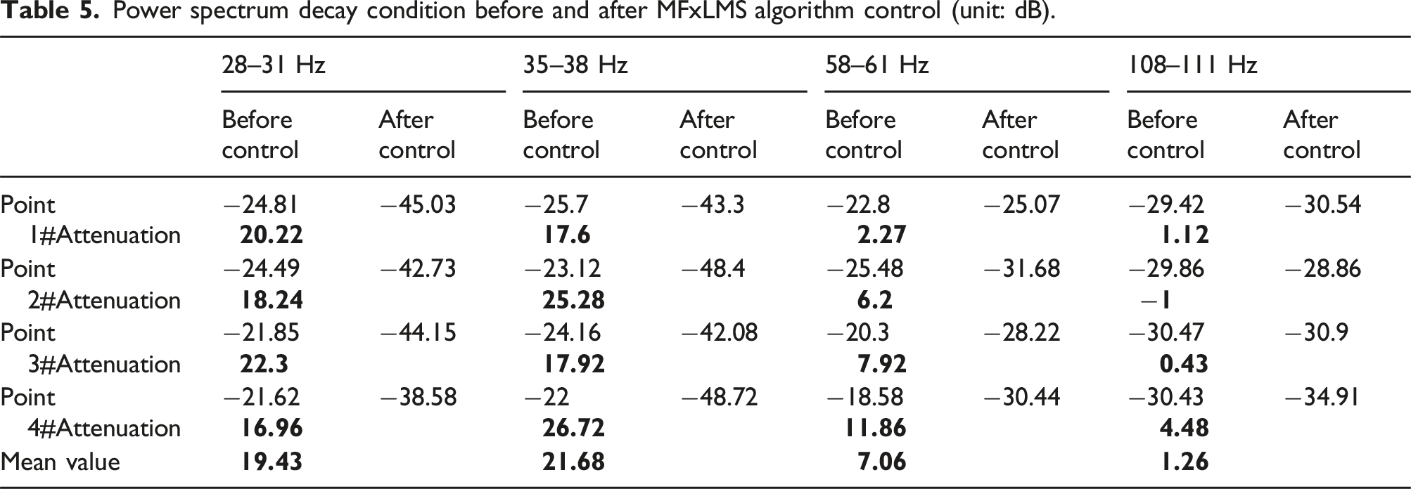
The experiment on active vibration isolation control using MFxLMS algorithm under fluctuating frequency spectral excitation is shown in Figure 20, which depicts the time history of the error signals at four measurement points and the power spectra before and after control. The active control begins at the 22nd second, resulting in a decrease in the error signal amplitude. The control stabilizes at around the 47th second, with a convergence time of 25 s. The power spectra reveal that the decline of the 28–31 Hz and 35–38 Hz spectral excitation is significant, with an average reduction of over 19 dB at the four measurement points. However, the control of the 58–61 Hz and 108–111 Hz spectral excitation is largely ineffective and even leads to an exacerbation of vibration. The specific control performance at each measurement point is shown in Table 5.

Figure 20.

Control effect of MFxLMS algorithm under sweep frequency excitation. (a) Time history diagram of error signal at measurement point 1#. (b) Power spectrum of error signal at measurement point 1#. (c) Time history diagram of error signal at measurement point 2#. (d) Power spectrum of error signal at measurement point 2#. (e) Time history diagram of error signal at measurement point 3#. (f) Power spectrum of error signal at measurement point 3#. (g) Time history diagram of error signal at measurement point 4#. (h) Power spectrum of error signal at measurement point 4#.

Table 5.

Power spectrum decay condition before and after MFxLMS algorithm control (unit: dB).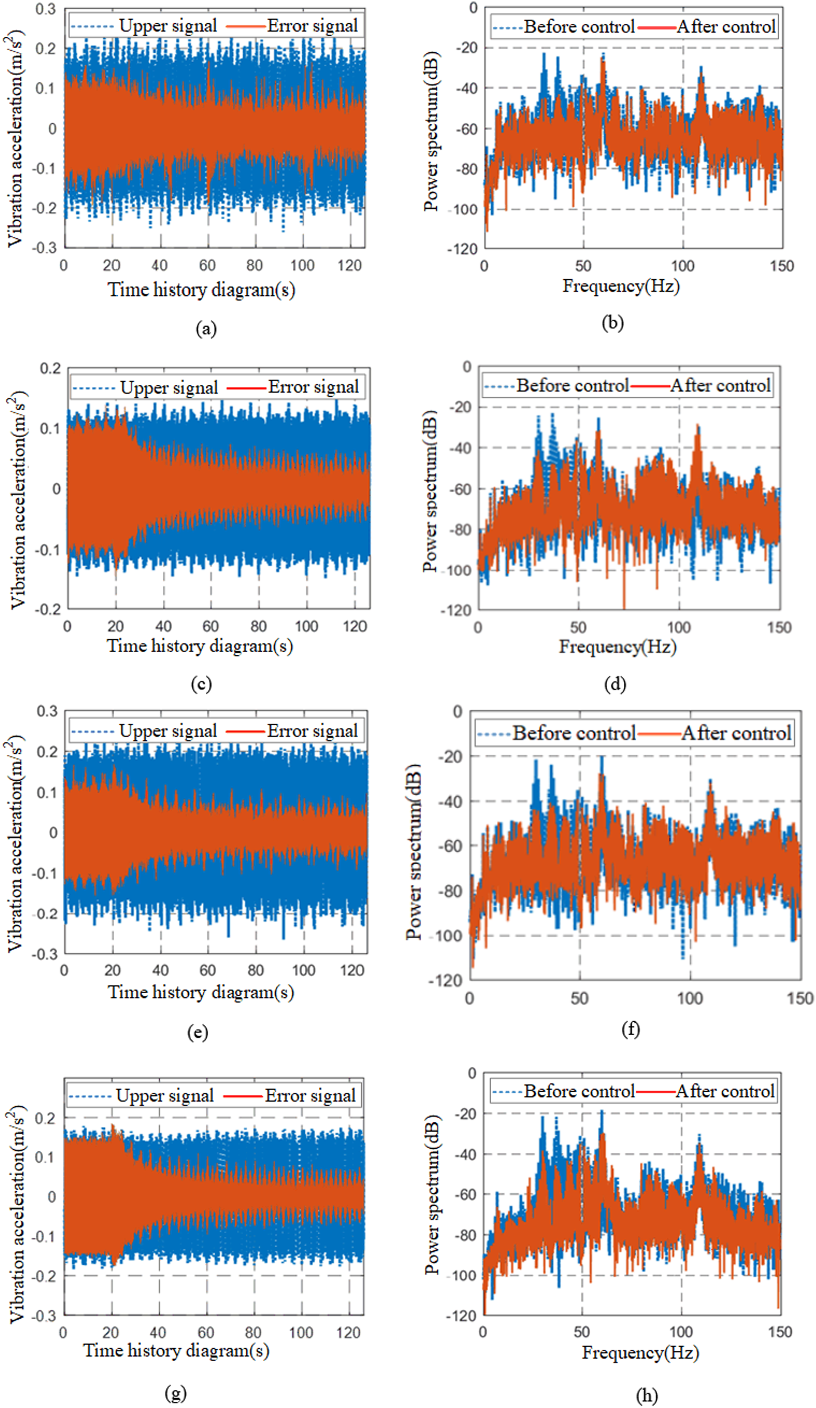

	28–31 Hz		35–38 Hz		58–61 Hz		108–111 Hz
	Before control	After control	Before control	After control	Before control	After control	Before control	After control
Point 1#Attenuation	−24.81	−45.03	−25.7	−43.3	−22.8	−25.07	−29.42	−30.54
Point 1#Attenuation	20.22		17.6		2.27		1.12
Point 2#Attenuation	−24.49	−42.73	−23.12	−48.4	−25.48	−31.68	−29.86	−28.86
Point 2#Attenuation	18.24		25.28		6.2		−1
Point 3#Attenuation	−21.85	−44.15	−24.16	−42.08	−20.3	−28.22	−30.47	−30.9
Point 3#Attenuation	22.3		17.92		7.92		0.43
Point 4#Attenuation	−21.62	−38.58	−22	−48.72	−18.58	−30.44	−30.43	−34.91
Point 4#Attenuation	16.96		26.72		11.86		4.48
Mean value	19.43		21.68		7.06		1.26

The secondary channels are coupled to their respective control circuits with weighting factors as compensation, as depicted in Figure 21. This figure displays the time history of the error signals and the power spectra before and after control at each of the four measurement points. The active control initiates at the 24th second and reaches convergence at the 25.5th second, achieving rapid convergence. The time history graph shows that the error signal amplitude after control can reduce up to 86%. The power spectra of the sweep frequency excitation at the four measurement points exhibit a noticeable decline, with the spectral signals after control effectively obscured by the background noise, and without inducing any oscillations at other frequencies. The specific control results can be seen in Table 6.

Figure 21.

Control performance of the DMFxLMS algorithm under sweep frequency excitation. (a) Time history diagram of error signal at measurement point 1#. (b) Power spectrum of error signal at measurement point 1#. (c) Time history diagram of error signal at measurement point 2#. (d) Power spectrum of error signal at measurement point 2#. (e) Time history diagram of error signal at measurement point 3#. (f) Power spectrum of error signal at measurement point 3#. (g) Time history diagram of error signal at measurement point 4#. (h) Power spectrum of error signal at measurement point 4#.

Table 6.

Power spectrum decay condition before and after DMFxLMS algorithm control (unit: dB).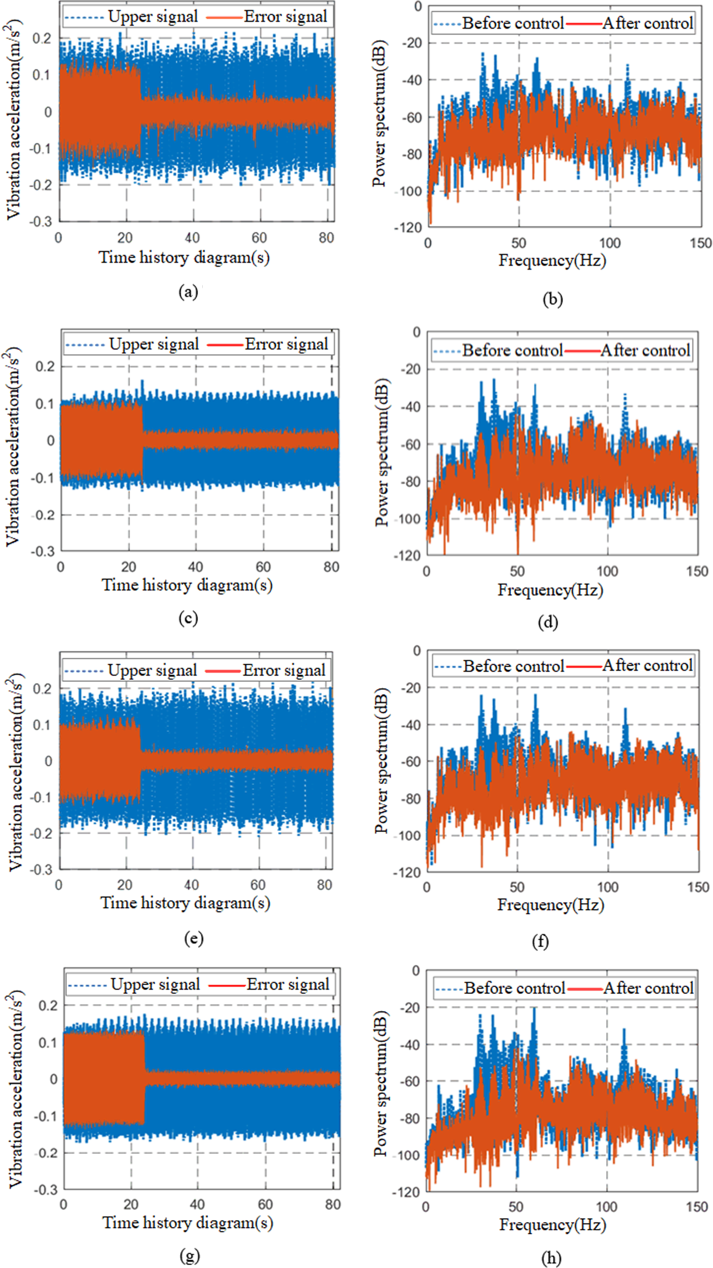

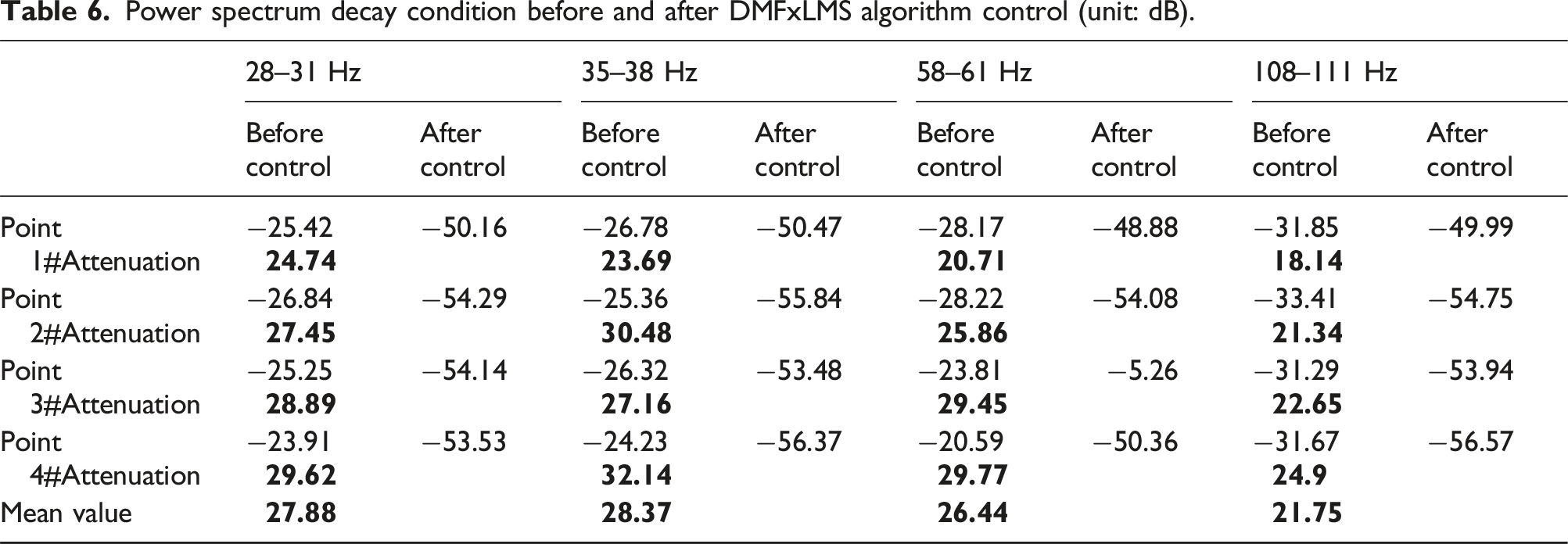
	28–31 Hz		35–38 Hz		58–61 Hz		108–111 Hz
	Before control	After control	Before control	After control	Before control	After control	Before control	After control
Point 1#Attenuation	−25.42	−50.16	−26.78	−50.47	−28.17	−48.88	−31.85	−49.99
Point 1#Attenuation	24.74		23.69		20.71		18.14
Point 2#Attenuation	−26.84	−54.29	−25.36	−55.84	−28.22	−54.08	−33.41	−54.75
Point 2#Attenuation	27.45		30.48		25.86		21.34
Point 3#Attenuation	−25.25	−54.14	−26.32	−53.48	−23.81	−5.26	−31.29	−53.94
Point 3#Attenuation	28.89		27.16		29.45		22.65
Point 4#Attenuation	−23.91	−53.53	−24.23	−56.37	−20.59	−50.36	−31.67	−56.57
Point 4#Attenuation	29.62		32.14		29.77		24.9
Mean value	27.88		28.37		26.44		21.75

Based on the analysis presented above, it can be inferred that:

(1) The decentralized decoupling optimization algorithm simplifies the system into parallel single-channel control circuits, reducing computational complexity and improving the performance of the four-channel control.

(2) The DMFxLMS algorithm significantly increases convergence speed, reducing the convergence time to just 1.8 s. The time delay compensation algorithm eliminates the effect of time delay on the control system. Compared to the MFxLMS algorithm, the decline in power spectral levels in each frequency band increases by 5–8 dB, further enhancing control accuracy. The decline in the power spectra of the sweep frequency spectra at 28–31 Hz, 35–38 Hz, 58–61 Hz, and 108–111 Hz can reach 27.88, 28.37, 26.44, and 21.75 dB, respectively, validating the efficacy of the algorithm.

Conclusion

This study focused on the vibration control of mechanical equipment in ships and aimed to design a control algorithm to address the challenges posed by multiple spectra, frequency fluctuations, slow convergence speed, multi-channel coupling, and poor stability. The following are the main conclusions of this study:

(1) The impact of secondary channel identification error on the control system was analyzed and a minimum least squares recursive identification algorithm with a forgetting factor was proposed. This algorithm demonstrated strong identification capabilities for secondary channel parameters and improved both the convergence speed and control accuracy;

(2) A decentralized decoupling approach was employed to eliminate the influence of secondary channels between the hybrid isolator and non-adjacent sensors in the algorithm. The compensation was provided in the form of feedback factors in each control circuit, reducing the system to a parallel single-channel control circuit and thereby improving the algorithm’s convergence performance;

(3) To address impacts caused by other mechanical equipment during the control process, an impact suppression factor was introduced into the control weight coefficient correction term. This ensured that the control weight coefficient remained stable during abrupt changes in the error signal. The output signal was suppressed using a percentage function to ensure quick stabilization during impacts;

(4) Simulation and experimental results confirmed that secondary channel coupling significantly impacted the convergence speed and vibration isolation effect of the control. The decentralized decoupling optimization algorithm effectively addressed the impact of coupling on control and demonstrated significant control results for both constant frequency spectra excitation and frequency fluctuation spectra excitation with fast convergence and good robustness.

Footnotes

Declaration of conflicting interests

The author(s) declared no potential conflicts of interest with respect to the research, authorship, and/or publication of this article.

Funding

The author(s) disclosed receipt of the following financial support for the research, authorship, and/or publication of this article: This work was supported by the National Natural Science Foundation of China (Grant No. 52201389 and 51679245); Natural Science Foundation of Hubei Province (Grant No. 2020CFB148).

ORCID iD

Kai Chai

References

Cheng

. A summary of acoustic characteristics and control techniques of underwater non-cavitation thruster. J Mech Eng Sci 2019; 233(18): 6339–6356.

Shen

Yang

, et al. Design of single degree-of-freedom optimally passive vibration isolation system. Journal of Vibration Engineering & Technologies 2015; 3(1): 25–36.

Daley

Zazas

. A recursive least squares-based control algorithm for the suppression of tonal disturbances. J Sound Vib 2012; 331(6): 1270–1290.

Widrow

Hoff

. Adaptive switching circuits[C]. Francisco, CA: Ire Wescon Conv Rec, 1966.

Fang

Zhu

Zhang

. A novel variable step size least mean square method for adaptive micro-vibration control. J Vib Control. 2022; 28(19–20): 2925–2939.

Burdisso

Nikolaidis

. Control of internal resonances in vibration isolators using passive and hybrid dynamic vibration absorbers. J Vib Control 2005; 286(4-5): 697–727.

Widrow

Sterarns

. Adaptive signal processing. International Softcover EditionBrand new, 1985. [M].

Kuo

Morgan

. Active noise control systems: algorithms and DSP implementations. New York, NY: John Wiley & Sons, 1996.

Chung

IKJ

. Multi-channel normalized FxLMS algorithm for active noise control. Journal of the Acoustical Society of Korea 2016; 35(4): 280–287.

10.

Aslam

Shi

Lim

. Variable threshold-based selective updating algorithms in feed-forward active noise control systems. IEEE Transactions on Circuits and Systems I-Regular Papers 2019; 66(2): 782–795.

11.

Qiu

Guo

. A generalized leaky FxLMS algorithm for tuning the waterbed effect of feedback active noise control systems. Mech Syst Signal Process 2018; 106: 13–23.

12.

Chung

IKJ

. A filtered-x affine projection sign algorithm with improved convergence rate for active impulsive noise control. Journal of the Acoustical Society of Korea 2015; 34(2): 130–137.

13.

Sun

Jiang

, et al. A variable momentum factor filtered-x weighted accumulated LMS algorithm for narrowband active noise control systems. Measurement 2014; 48: 282–291.

14.

Chang

Chu

. Feedforward active noise control with a new variable tap-length and step-size Filtered-x LMS algorithm. IEEE-ACM Transactions on Audio Speech and Language Processing 2014; 22(2): 542–555.

15.

Mazur

Schroder

Andrekson

. Joint superchannel digital signal processing for effective inter-channel interference cancellation. J Lightwave Technol 2020; 38(20): 5676–5684.

16.

Deligiannis

Mota

JFC

Andreopoulos

, et al. Fast desynchronization for decentralized multichannel medium access control. IEEE Trans Commun 2015; 63(9): 3336–3349.

17.

Kim

Elliott

Brennan

. Decentralized control for multichannel active vibration isolation. IEEE Trans Control Syst Technol 2001; 9(1): 93–100.

18.

Liu

Morse

. Structural completeness of a multichannel linear system with dependent parameters. IEEE Trans Automat Control 2022; 67(1): 267–278.

19.

Chen

. A fast vibration-level adjustment method for low-frequency vibration calibration based on modified filtered-x least mean square algorithm. Measurement & Control 2020; 53(3-4): 328–338.

20.

Zhou

Zou

Qiu

. A frequency band constrained filtered-x least mean square algorithm for feedback active control systems. J Acoust Soc Am 2020; 148(4): 1947–1951.

21.

George

Panda

. On the development of adaptive hybrid active noise control system for effective mitigation of nonlinear noise. Signal Process 2012; 92(2): 509–516.

22.

Wang

Shuai

, et al. A multi-reference filtered-x-Newton narrowband algorithm for active isolation of vibration and experimental investigations. Mech Syst Signal Process 2018; 98: 108–123.

23.

Shu

. Online secondary path modeling method with auxiliary noise power scheduling strategy for multi-channel adaptive active noise control system. J Low Freq Noise Vib Act Control 2019; 38(2): 740–752.

24.

Zhou

Chen

Meng

, et al. A modified filtered-x least mean square/fourth algorithm using weighted reference signal for active noise control. Int J Adapt Control Signal Process 2022; 36(4): 882–900.

25.

DeBrunner

Wang

. Sub-band adaptive filtering with delay compensation for active control. IEEE Trans Signal Process 2004; 52(10): 2932–2937.

26.

Gao

Guo

Liu

, et al. Method for online identification of secondary path based on wavelet transform. Journal of University of Science & Technology (Natural Science Edition) 2020; 48(9): 89–94, (in Chinese).

27.

. Active noise cancellation algorithms for impulsive noise. Mech Syst Signal Process 2013; 36(2): 630–635.

28.

Arablouei

Dogancay

. Reduced-complexity constrained recursive least-squares adaptive filtering algorithm. IEEE Trans Signal Process 2012; 60(12): 6687–6692.

29.

Liu

Sun

Jiang

. Kernel filtered-x LMS algorithm for active noise control system with nonlinear primary path. Circ Syst Signal Process 2018; 37(12): 5576–5594.

30.

Chu

Zhao

Niu

, et al. Wind noise suppression in filtered-x least mean squares-based active noise control systems. J Acoust Soc Am 2022; 152(6): 3340–3345.

31.

Zhang

. Eigenvalue inequalities for matrix product. IEEE Trans Automat Control 2006; 51(9): 1506–1509.

32.

Chai

Liu

Gao

, et al. Hartley block algorithm and experiment in adaptive control. J Natl Univ Def Technol. 2023; 45(1): 174–184.

Multi-channel decentralized decoupling FxLMS algorithm and active vibration control experiment

Abstract

Keywords

Introduction

Basic FxLMS theory and least squares recursive identification algorithm

Basic FxLMS theory

Recursive least squares identification algorithm

Algorithm principle

Numerical simulation

Multi-channel decentralized FxLMS algorithm and design of anti-shock circuit

Multi-channel decentralized FxLMS algorithm

Design of anti-impact link

Impact mitigation factor

Output saturation mitigation

Simulation analysis

Experimental research

Development of the NI-PXIe control system and isolation test bed

Offline identification of primary and secondary channels

Isolation control experiment and analysis

Fixed-frequency spectrum excitation active control experiment

Experiment on active control with fluctuating frequency spectral excitation

Conclusion

Footnotes

Declaration of conflicting interests

Funding

ORCID iD

References