
Abstract
In this article, we introduce a nonlinear oscillator equation containing two strong linear terms. An approximate solution was obtained using power series approach. Furthermore, by introducing a parameter to the original equation, we fined the fixed points of the modified nonlinear oscillator equation and study stability analysis of these fixed points. On the other hand, we simulate the solution of the nonlinear oscillator equation and introduced many plots for different initial conditions. Finally, we make some plots concerning the phase portrait for different cases.
Keywords
Introduction
Nonlinear oscillator differential equations arise in many branches in science as physics, structures, and engineering. Studying these equations are a prominent topic for researchers. In literature, a lot of efforts have been paid on studying them and there are many techniques (analytical and numerical) that have been introduced and used to solve such systems.1–9 Some researchers have presented several techniques for solving analytically a second order differential equation with various strong nonlinear terms. For example, Belhaq and Lakrad 6 used the multiple scales method for solving strongly nonlinear oscillators, and the variational approach and the Hamiltonian approach to nonlinear oscillators are systematically discussed in Refs. 10 and 11. The elliptic-harmonic-balance method is used to study mixed parity nonlinear oscillators. 7 Yuste and Bejarano 3 developed an elliptic Krylov–Bogolubov method with Jacobian elliptic functions for solving a differential equation with cubic nonlinearity. An averaging method using generalized harmonic functions for strongly nonlinear oscillators is presented in the paper of Xu and Cheung. 5
Several important oscillators with important applications in physics and engineering have attracted the attention of many researches.12–17 For example, the excited spring pendulum has been studied well using the so-called multi-scale method, in which the authors obtained approximate solutions of the equations of motion of the system.12,13 Furthermore, the Van-der Pol and Duffing oscillators have been considered in many works.13–17 In these references, one can see that the Van-der Pol oscillator was analyzed using some perturbation techniques to obtain approximate solution to its dynamical equations.14,15 On the other hand, the Duffing oscillator was also investigated in Refs. 14–17 where the authors used an effective analytical method to obtain the solution of it and compared it with a numerical solution using the forth-order Runge–Ktta method.
In He’s paper, 18 the author reviewed some simplest methods for fast calculation of the frequency–amplitude relationship of nonlinear oscillators. In addition to the previous works, many other methods have been applied to nonlinear oscillators. Also, in Ref. 19, He suggested a Hamiltonian approach to study nonlinear oscillators. In Ref. 20, homotopy perturbation method has been used to analyze non-conservative oscillators.
Investigating and studying the nonlinear oscillators is of great importance to a wide range of researchers. Many approximation methods have been commonly used for solving nonlinear equations. Perturbative and non-perturbative methods have been invented and applied in frequency, response, and stability analysis of nonlinear oscillators. These methods were also extended to include different fields of mechanics, specially in structural dynamics20–24 and fluid mechanics.25–27 Some of these methods include the energy balance method,28–36 the Hamiltonian approach and perturbation method20,37,38 in addition to the variational approach,39–42 and many others.
In Ref. 8, the exact solutions for the hard singular nonlinear oscillators are determined. All the methods mentioned above have their own advantages for obtaining approximate analytical solutions for a one-degree-of-freedom oscillator.
In a previous work, we find an exact solution for nonlinear oscillator with damped mass system by finding the potential function and make modification of the initial value studying a nonlinear differential equation and plotting some simulation plots for suggested initial conditions. 43 Another discussion of the solution for nonlinear oscillator is given in Refs. 43–45.
In this paper, we used power series method in solving differential equation containing third and fifth nonlinear terms as presented in Section 2. In Section 3, we make some analysis for fixed points and their stability. Results and discussions have been given in Section 4, and finally we close the paper by a conclusion section.
Power series solution for nonlinear oscillators
Consider the following nonlinear differential equation


This equation appears in Ref. 46 where the authors study it using homotopy perturbation method. Our purpose here is to obtain an exact solution for the above equation using power series concept, see Ref. 47. For this purpose, let the solution of the differential equation (2.1) be
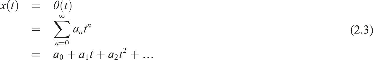
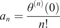

Now
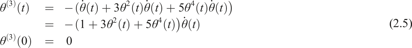

The fifth and sixth derivatives are required to make induction for the series solution. Thus, we have


Using the assumption (2.3) and equations (2.4)–(2.8), we get the solution of the differential equation (2.1) as follow:
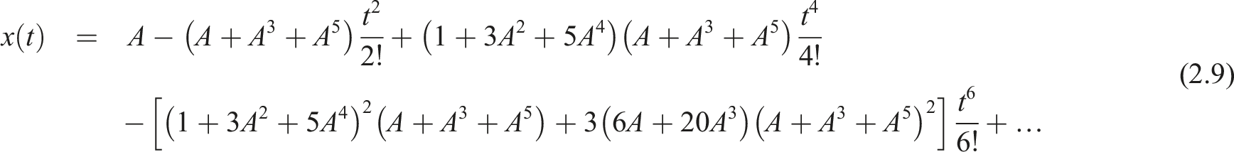
The solution (2.9) can be written as
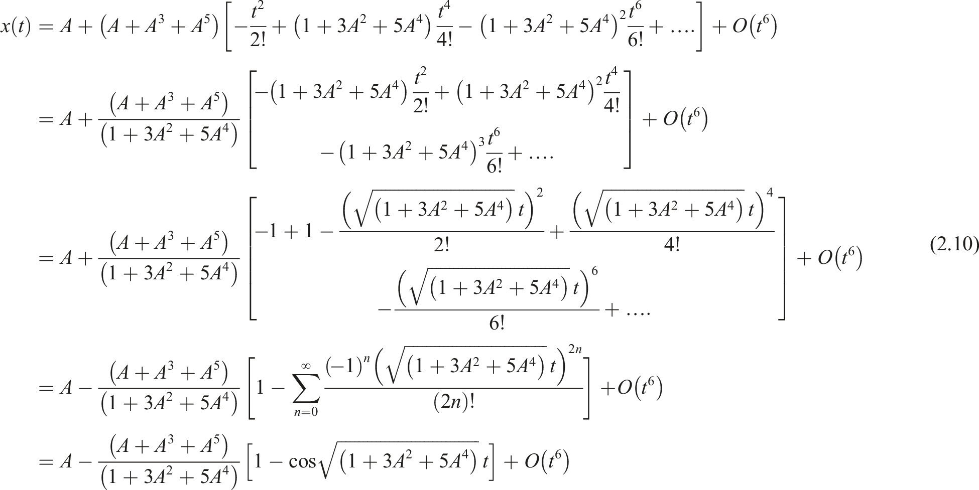
Ignoring solution error terms O(t6) leads to

Fixed points and stability analysis for nonlinear oscillator
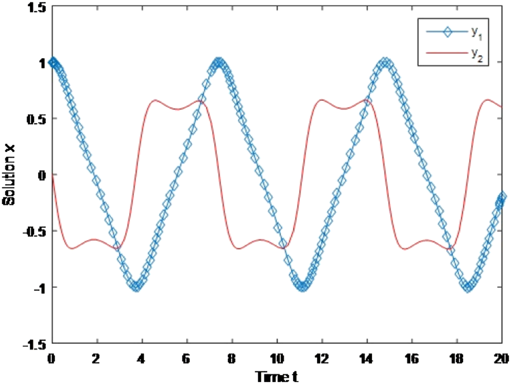
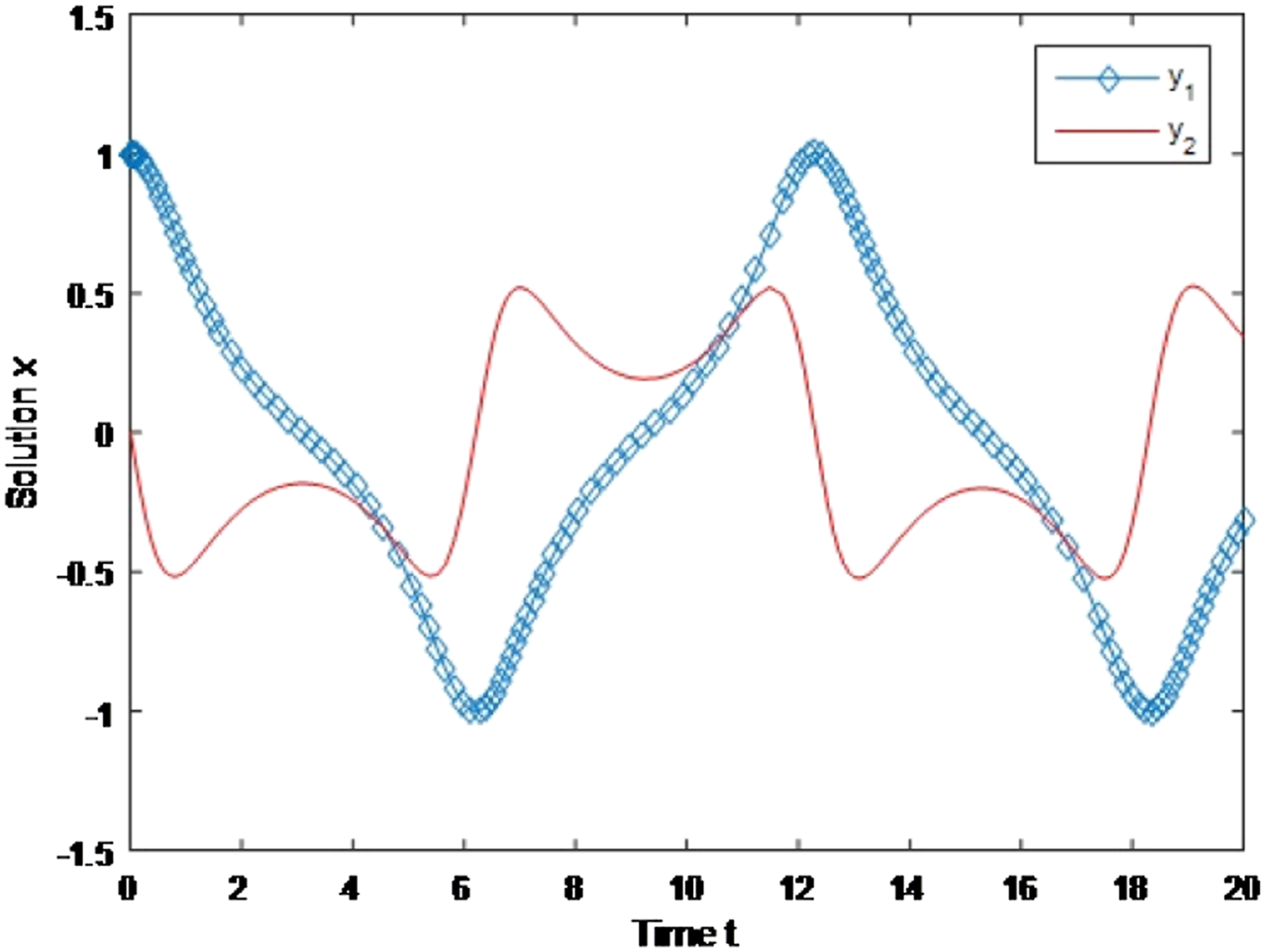
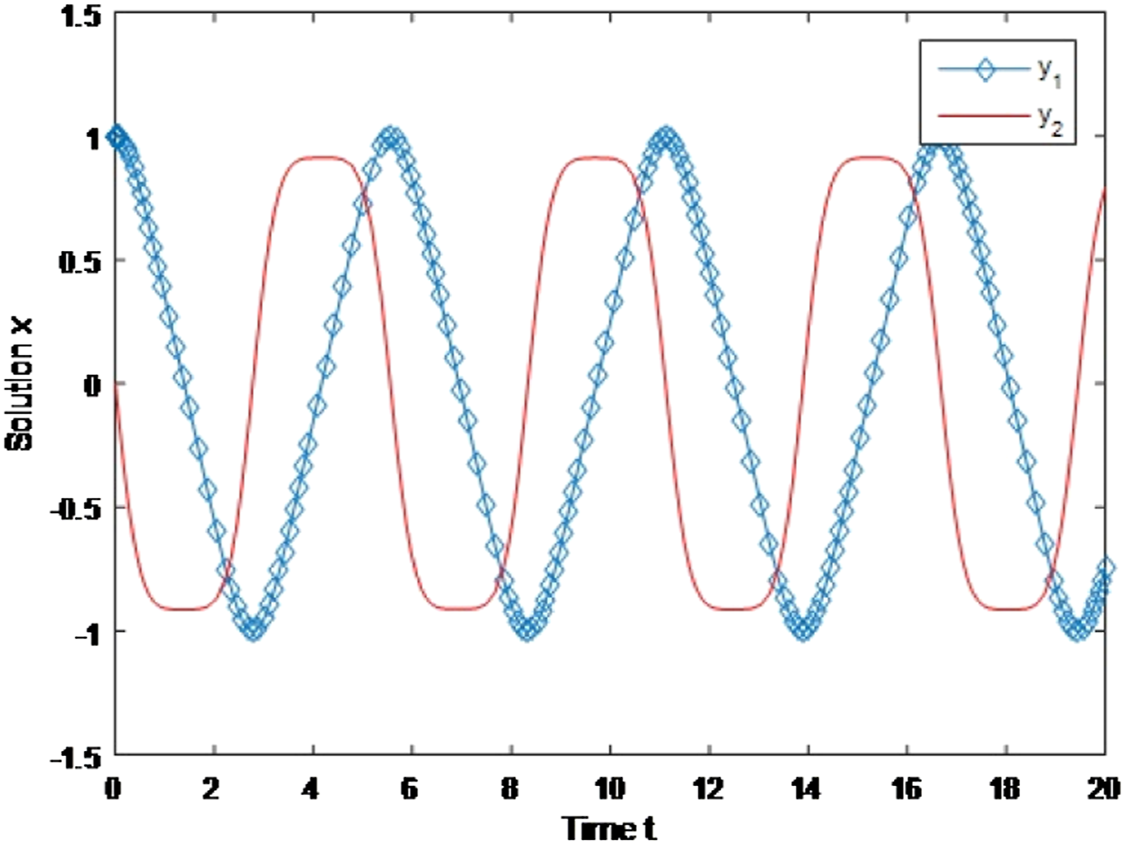
Equation (2.1) can be rewritten by multiplying the linear term with the parameter α to see its effect in the fixed points and its bifurcation. Thus Comparison of the approximate solution with numerical one for the case α = 1.0. Comparison of the approximate solution with numerical one for the case α = −0.5. Comparison of the approximate solution with numerical one for the case α = −0.8. Comparison of the approximate solution with numerical one for the case α = 0.0.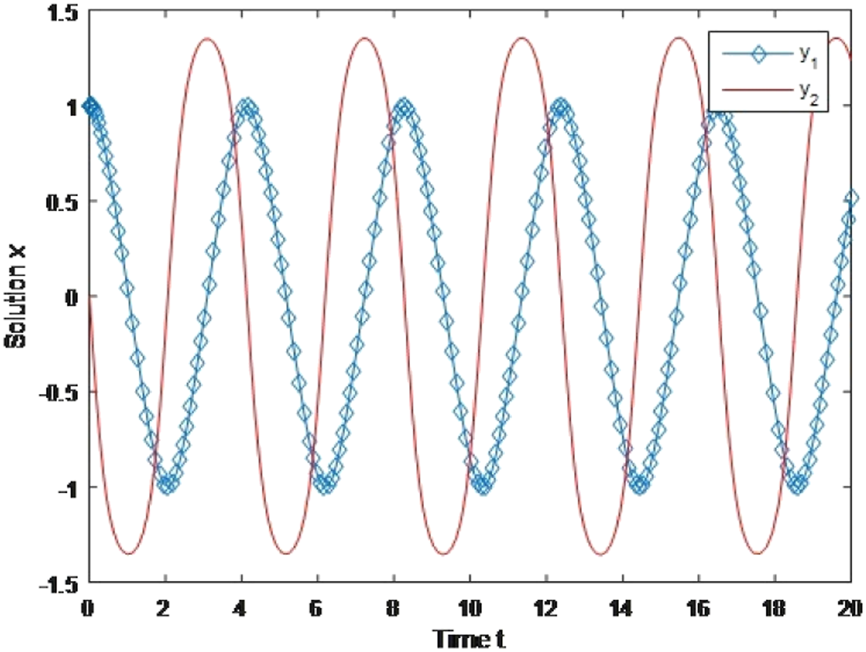

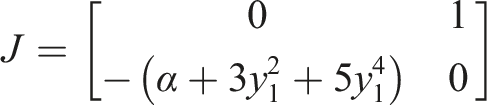
Now, in the following steps, we aimed to convert the system into two differential equations. So letting y1 = x and

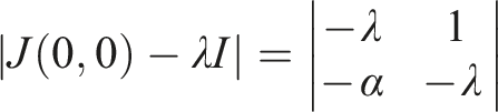
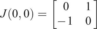
To find the fixed points for this continuous time model, take

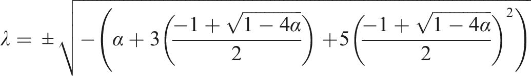
One can see that we have two fixed points, the first one is (y1, y2) = (0, 0), and when −1/4 ≤ α ≤ 0, we have another fixed point which depends on the value of α, and it is equal to
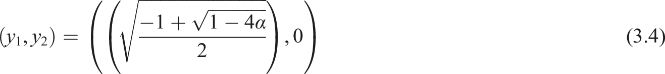
So
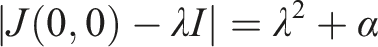
Since
Considering the secon0064 fixed point (3.4), we have
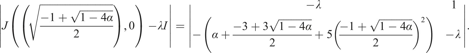
This implies that
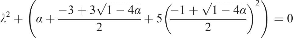

We have semistable fixed point as shown in inequality (3.5), while spiral fixed point happened as given in inequality (3.6).

Analyzing the stability using simulation for the fixed points through the spiral movement, since we have second order differential equation, the trajectories in the direction field will go to limit cycle where it become stable in some cases and unstable in others. We can have a periodic limit cycle that take all possible value about phase space around each fixed point through the intervals in (3.5) and (3.6) (for more information, see Ref. 47).
From Figure 5, we reach a stable limit cycle when we get close to the interval 0 ≤ α ≤ 1/4 and interval given in (3.5) while the solution become unstable when α satisfy the inequality in (3.6). Now, when taking values out of interval 0 ≤ α ≤ 1/4, it appear that there are two fixed points in the interval (3.5) that reach to stable limit cycle, while out of this interval, we have unstable limit cycle, see Figure 6. Limit cycle for the nonlinear oscillator (3.5) with α = 0.2 near the interval, 0 ≤ α ≤ 1/4. Limit cycle for the nonlinear oscillator (3.6) with α = 2 out of the interval 0 ≤ α ≤ 1/4.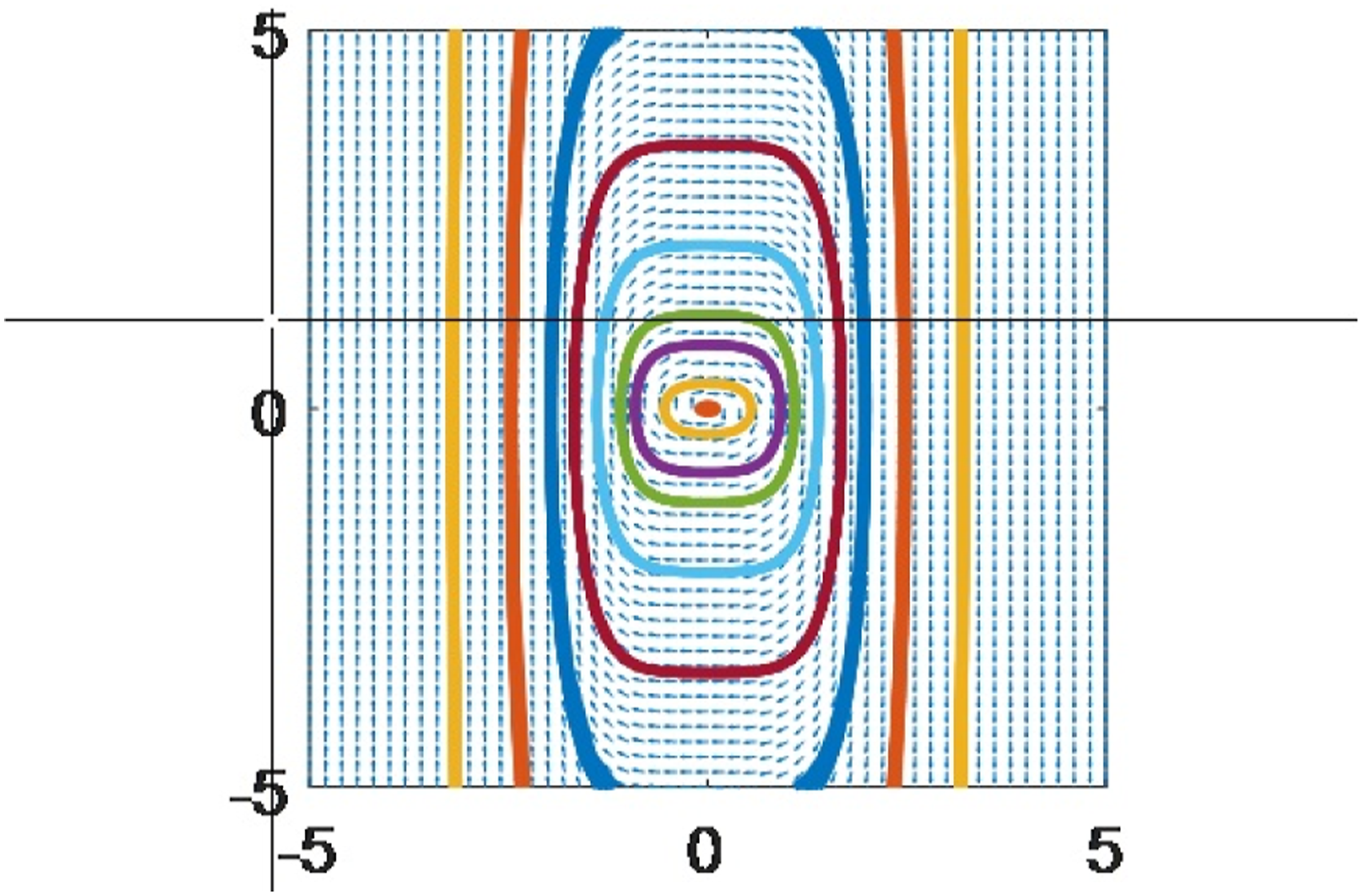
In general, we see that the system go toward two fixed points as we see theoretically, by finding the two fixed points (0,0), Limit cycle for the nonlinear oscillator (3.2) with α = −10. Limit cycle for the nonlinear oscillator (3.2) with α = 10.
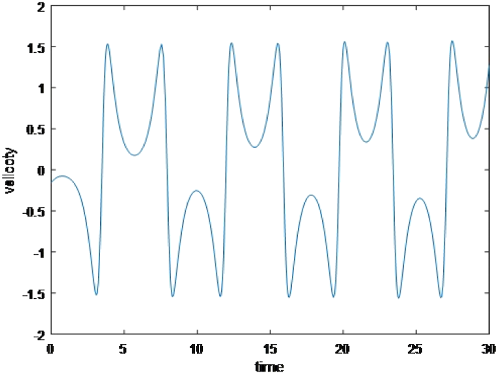
In the interval where there are two fixed points, the velocity and distance will be as shown in Figures 9 and 10 taken at α = −3 arbitrary as negative value. Variation of distance against time for the system (3.2) with α = −3. Variation of velocity against time for the system (3.2) with α = −3.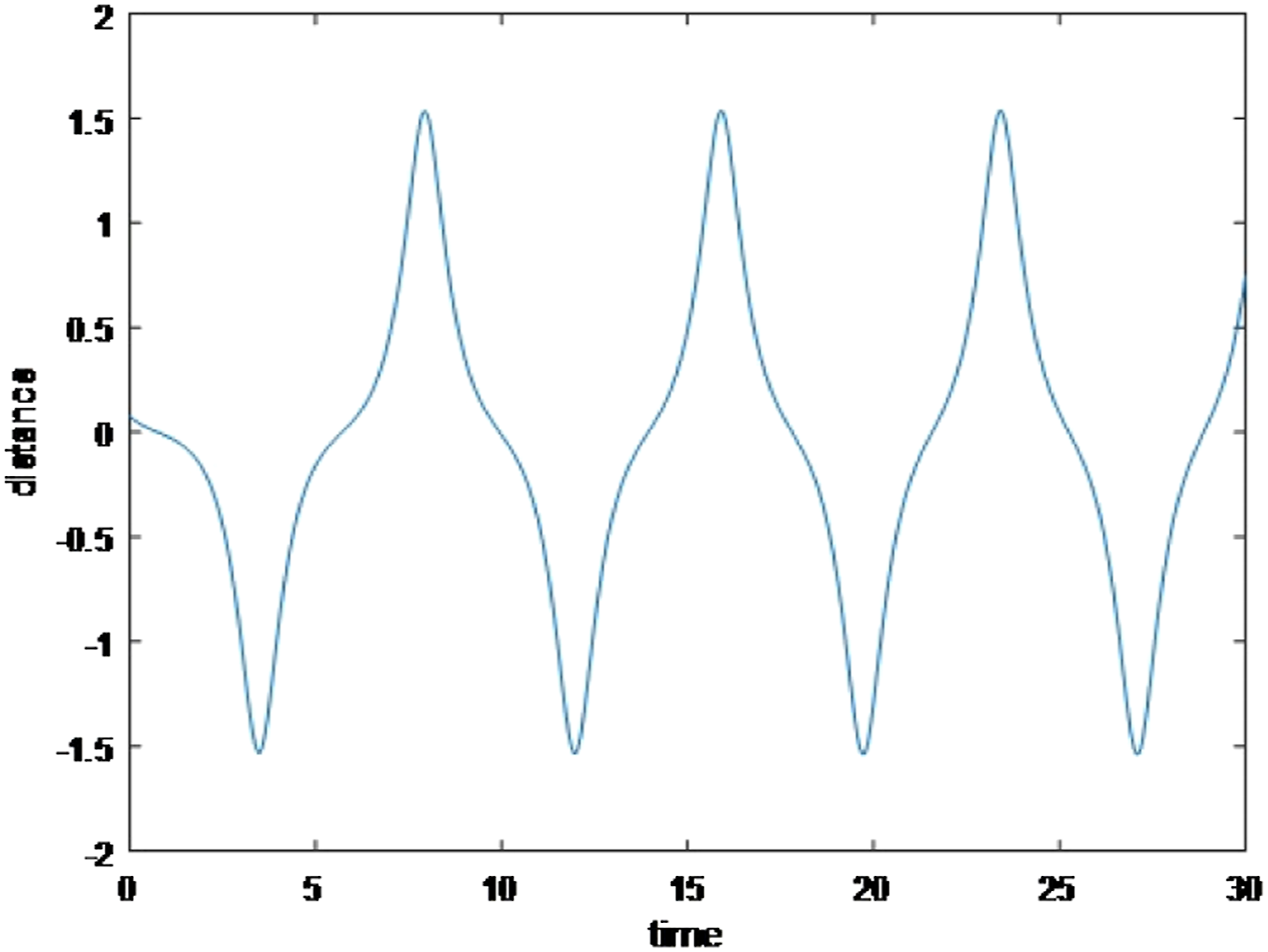
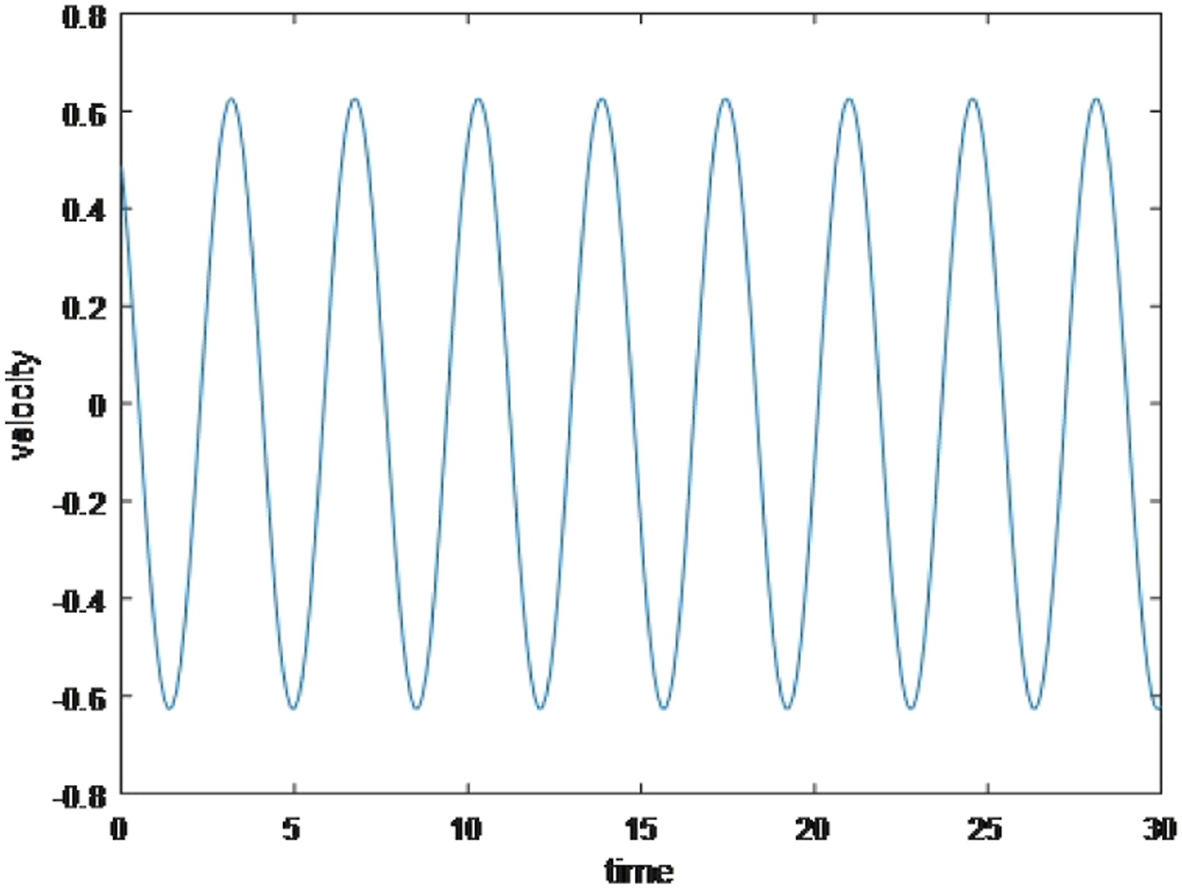
In addition, in the interval where there is only one fixed point, the velocity and distance will be as shown in Figures 11 and 12 taken at α = 3 arbitrary as positive value. Variation of distance against time for the system (3.2) with α = 3. Variation of velocity against time for the system (3.2) with α=3.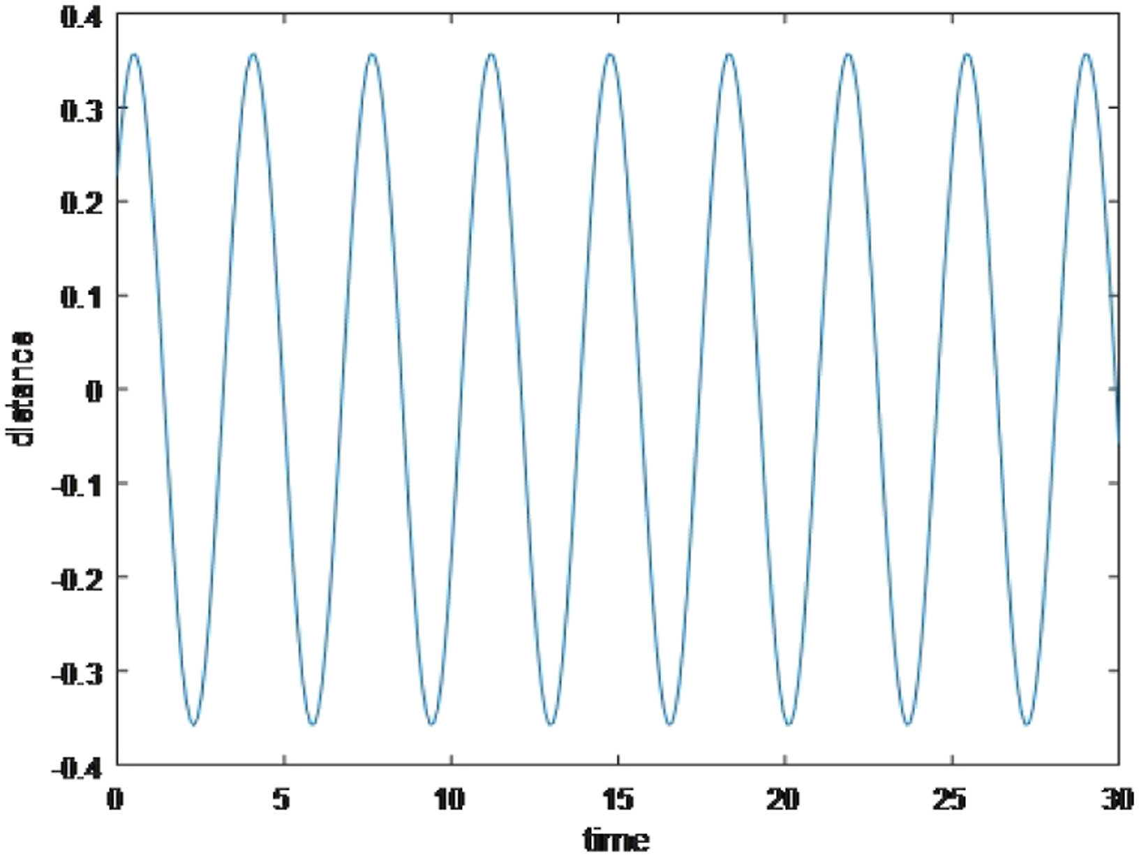
Visualizing three components of nonlinear oscillator time, distance, and velocity shown in the interval where the system have two fixed points as shown in Figure 13. Three dimension graph for simulation of the system (3.2) with two fixed points with α = 3.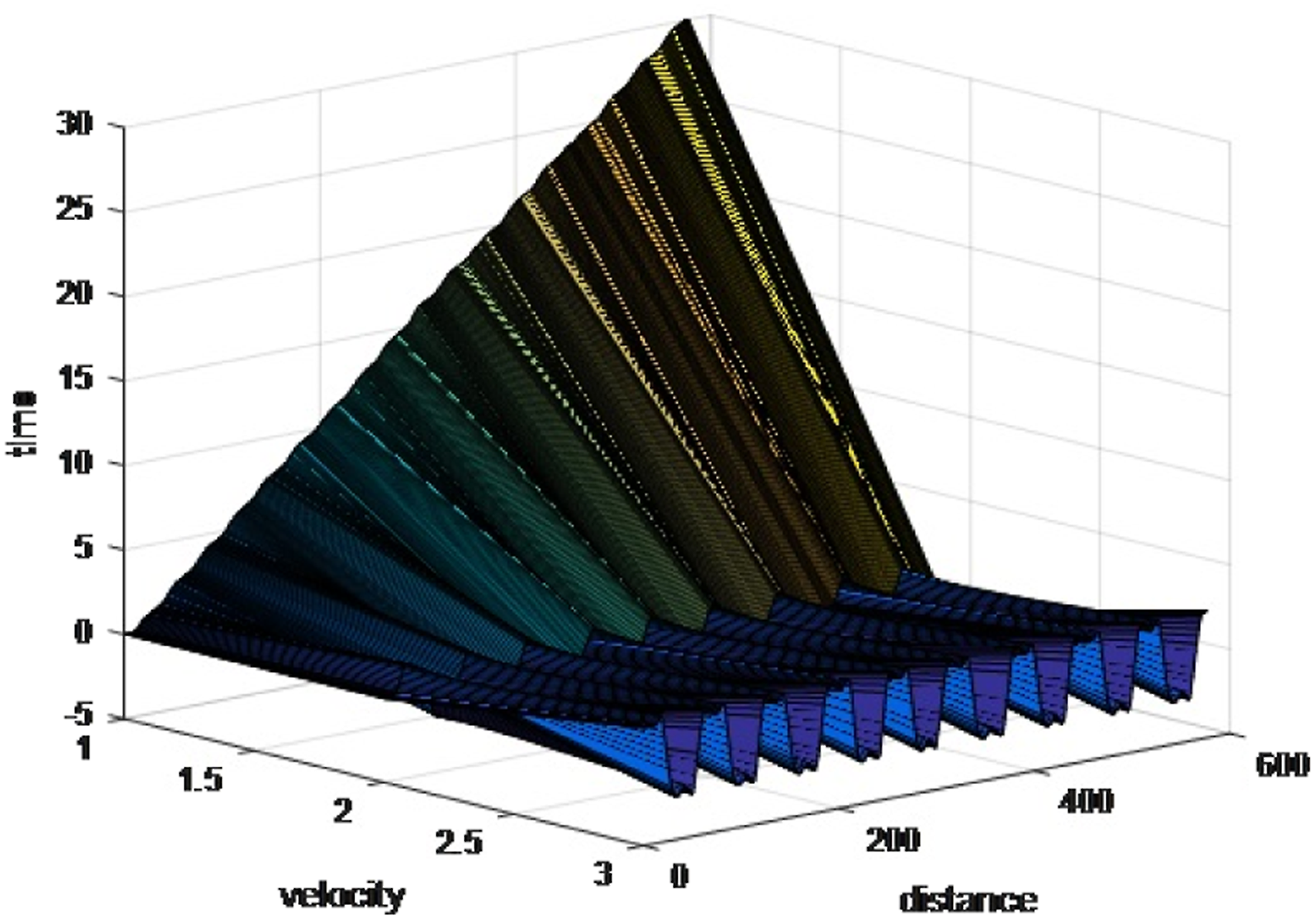
Now the system has one fixed point as shown in Figure 14. Three dimension graph for simulation of the system (3.2) with one fixed points α = 3.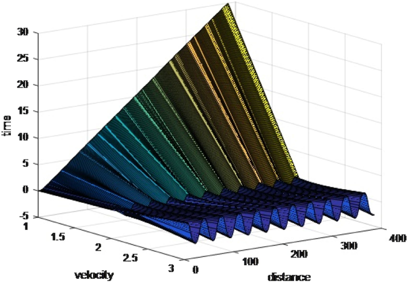
The system has steady oscillation in some interval while it goes so far away from fixed point in other side.
Analyzing one of general form for nonlinear oscillator
In many previous works 48,49 an approximate solution for nonlinear oscillator for some general forms, we are going heir to make numerical approach for the differential equation in the form


This geometric series converge when |x|<1 equation (4.2) and convert to the following form:

Multiplying equation (4.3) by
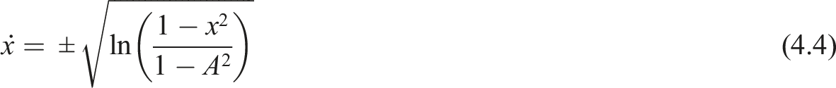
From equation (4.4), we need the positive value for periodic time, take the value
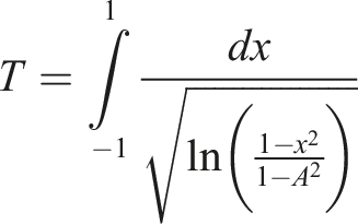
This improper integral can be evaluated numerically. Use this value in the explicit solution we take from equation (2.11) to get the frequency of the oscillator


We see that the accurate frequency we get from our solution in equation (2.11) is


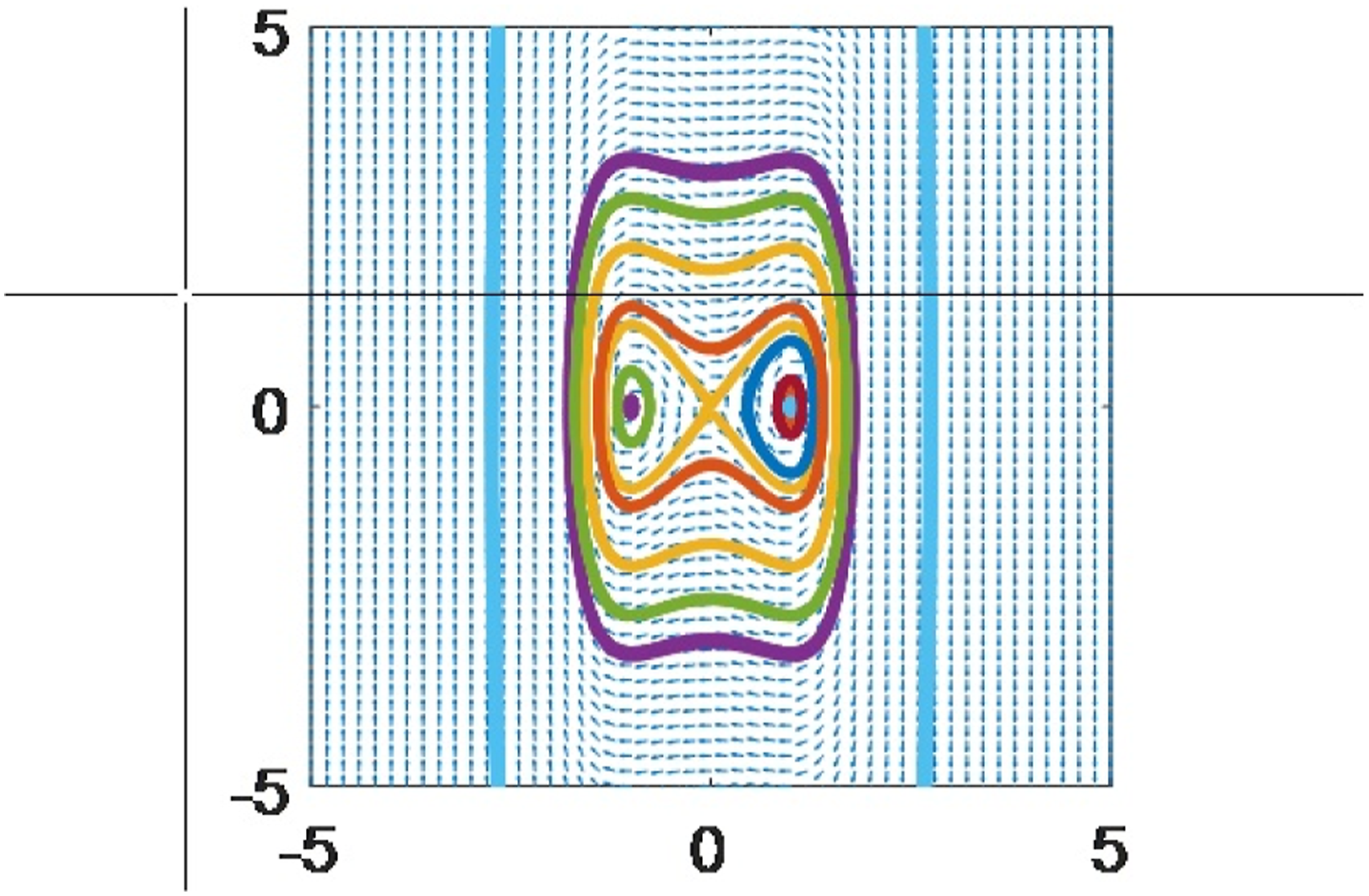
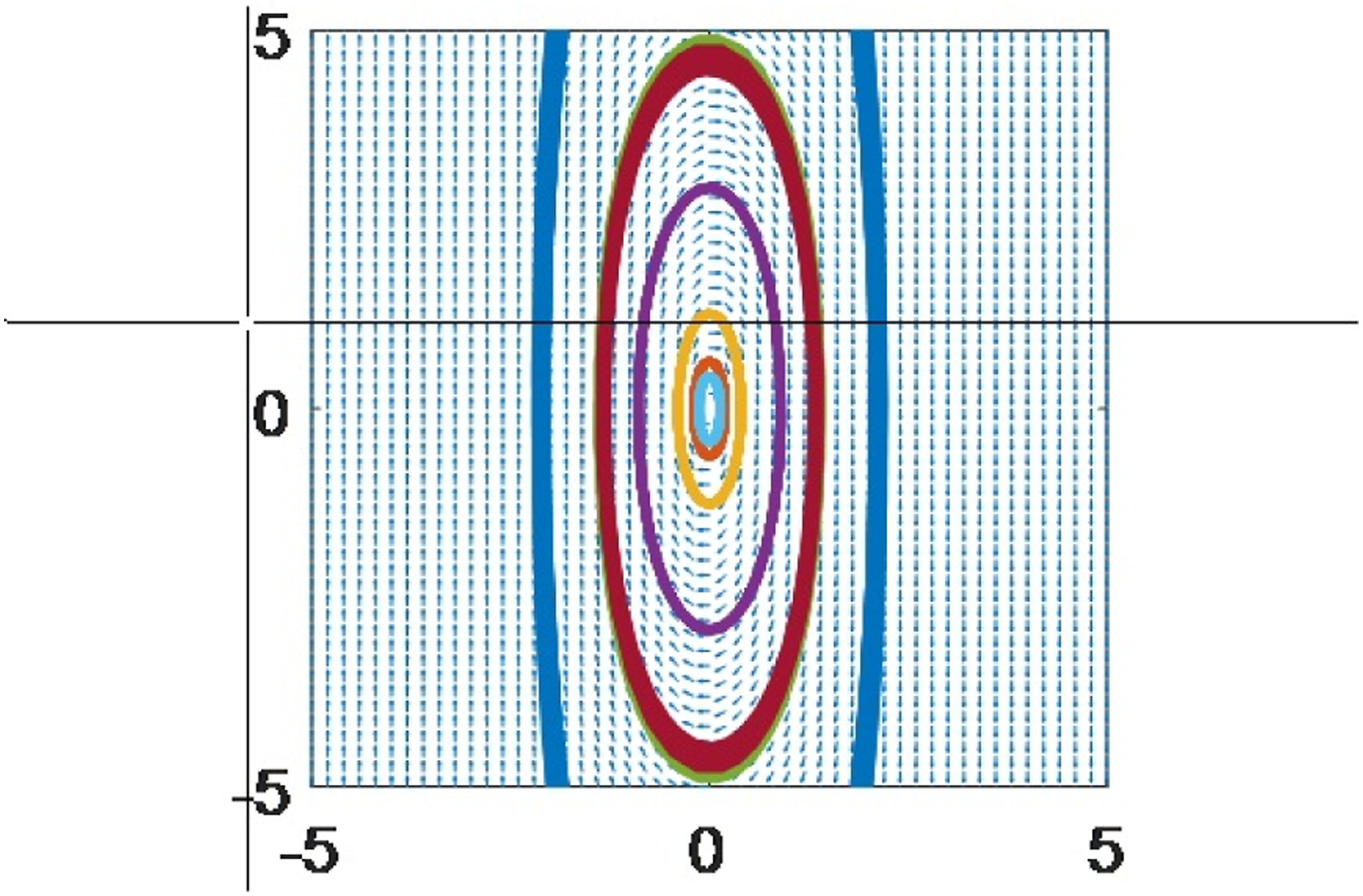
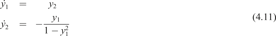
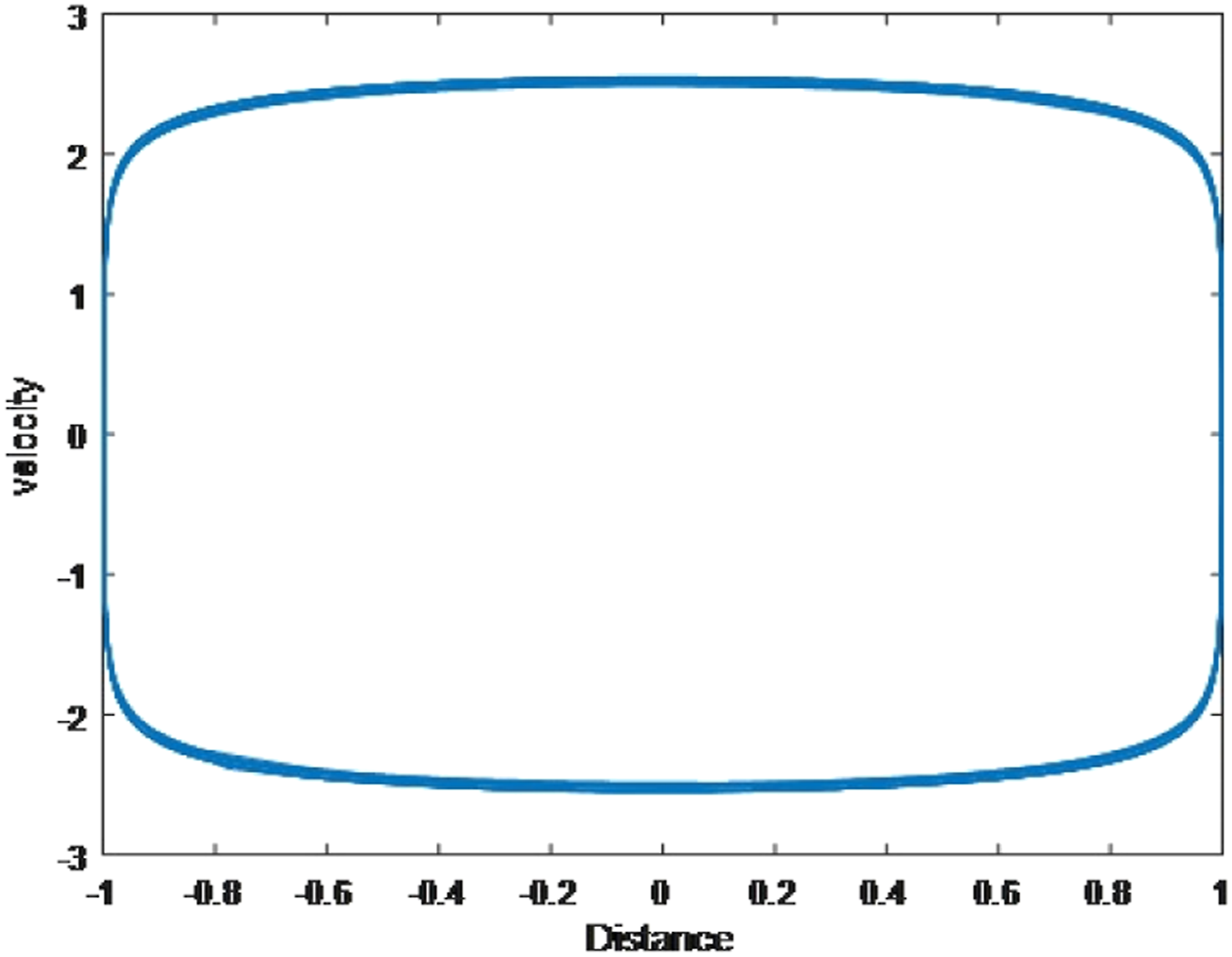
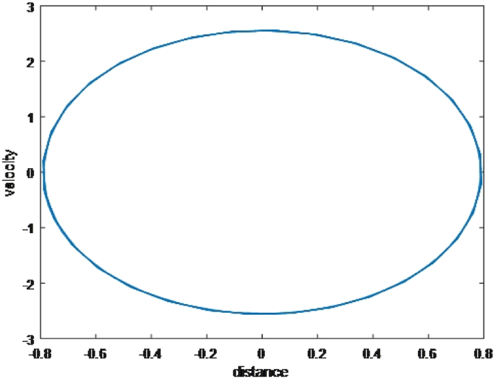
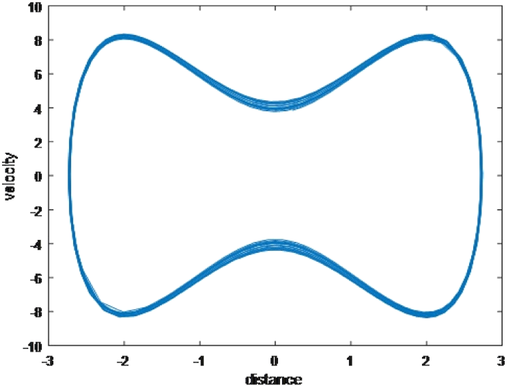
In our research, we have frequency–amplitude relation from the exact power solution when n = 2 and a periodicity for infinite non-linear terms, this case is considered in our analysis by converting equation (4.3) to the system Phase portrait for the nonlinear oscillator system (4.11) with A = 0.01. Phase portrait for the nonlinear oscillator system (4.11) with A = 1 × 10⁻⁵. Phase portrait for the nonlinear oscillator system (4.11) with A = 1 × 10⁻⁶ and time interval [−3, 3]. Phase portrait for the nonlinear oscillator system (4.11) with A = 1 × 10⁻⁵ and time interval [−6, 6].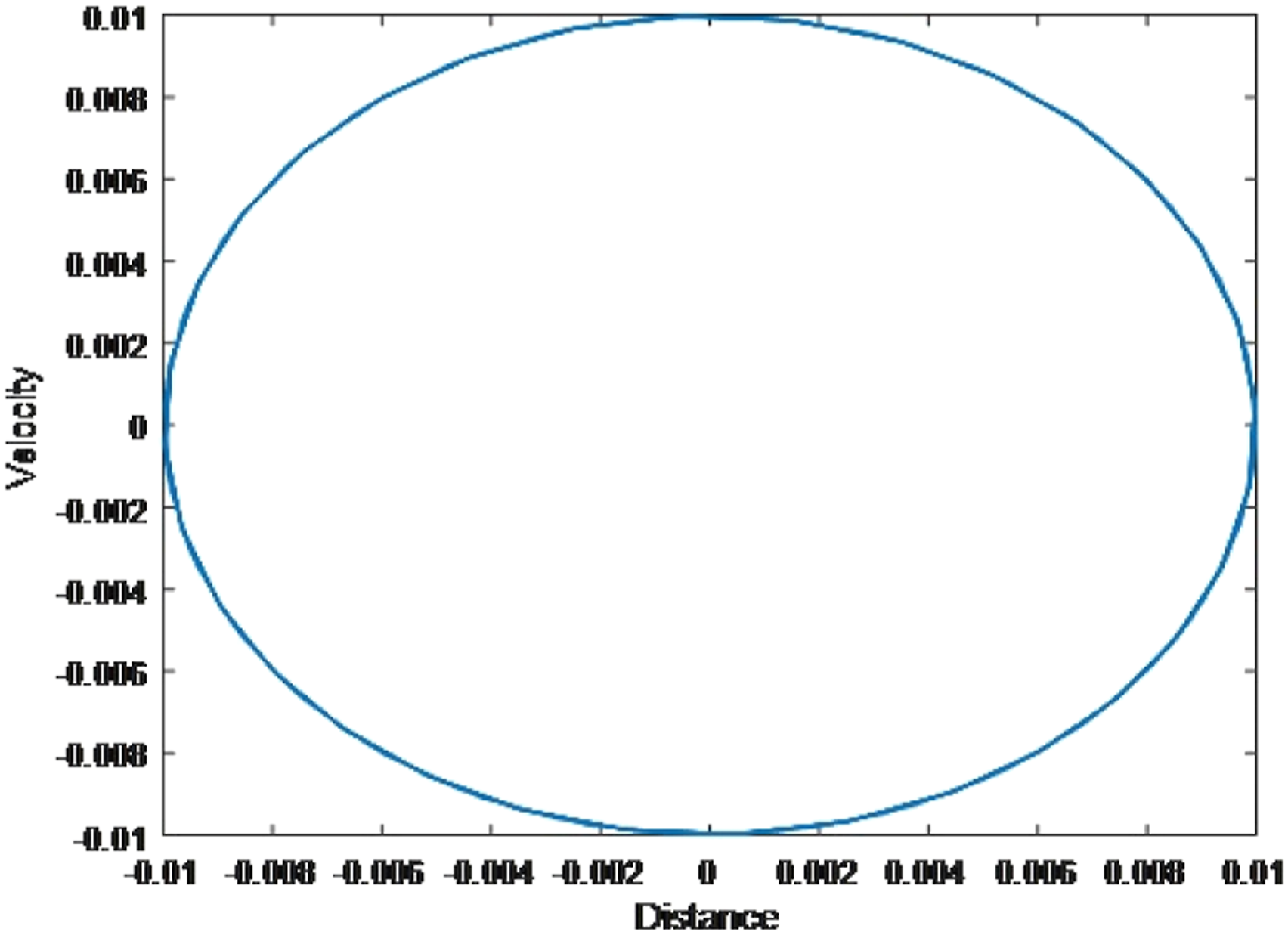
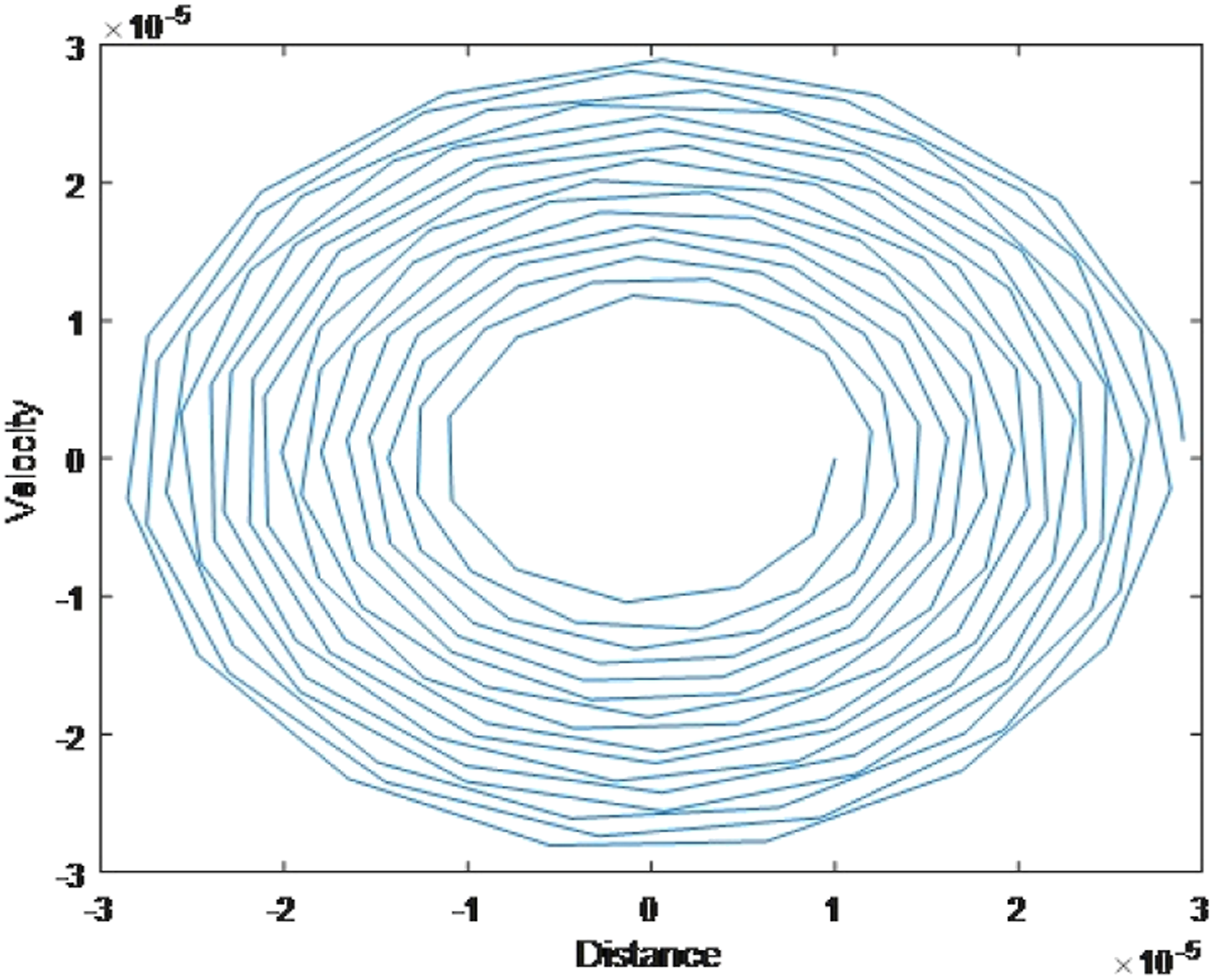
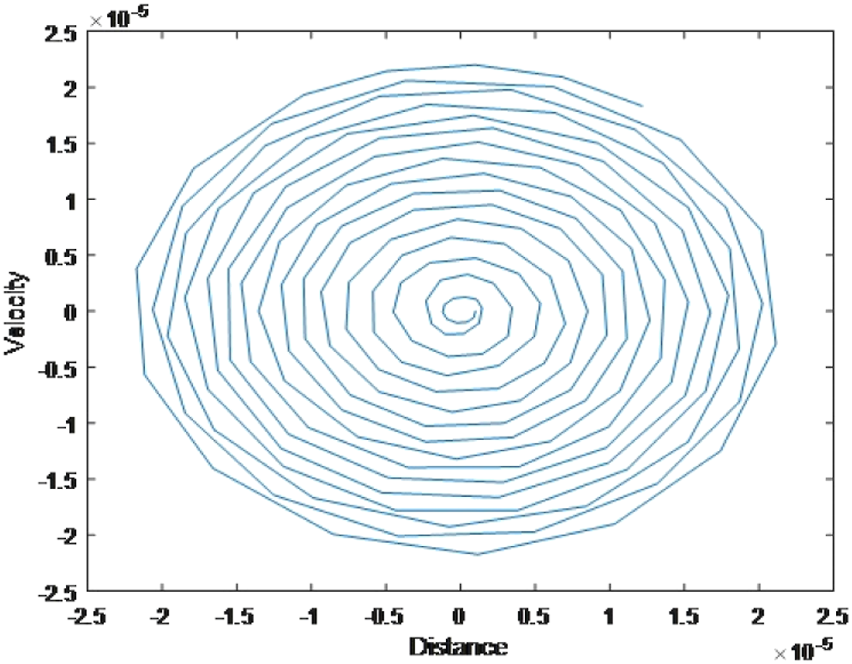
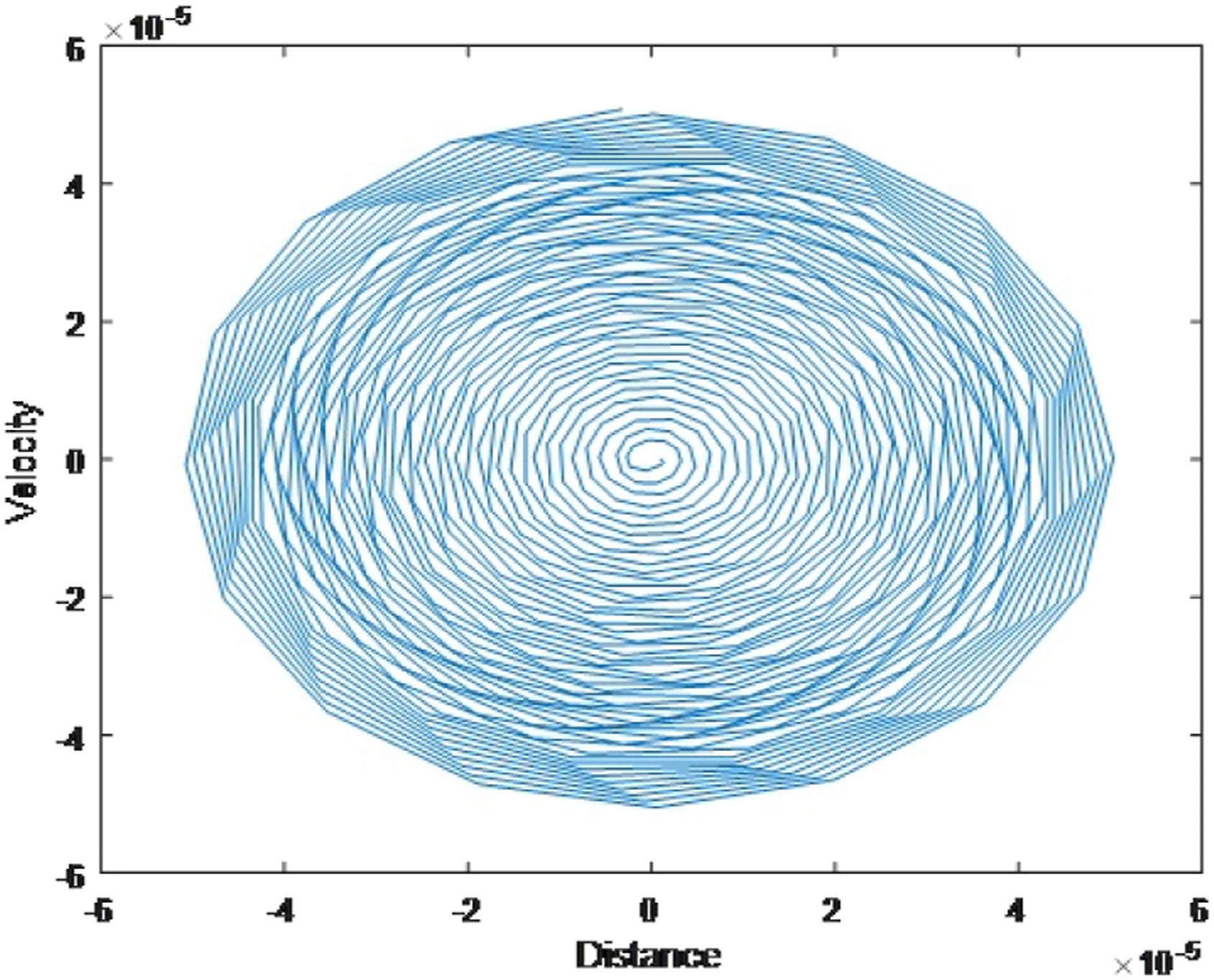
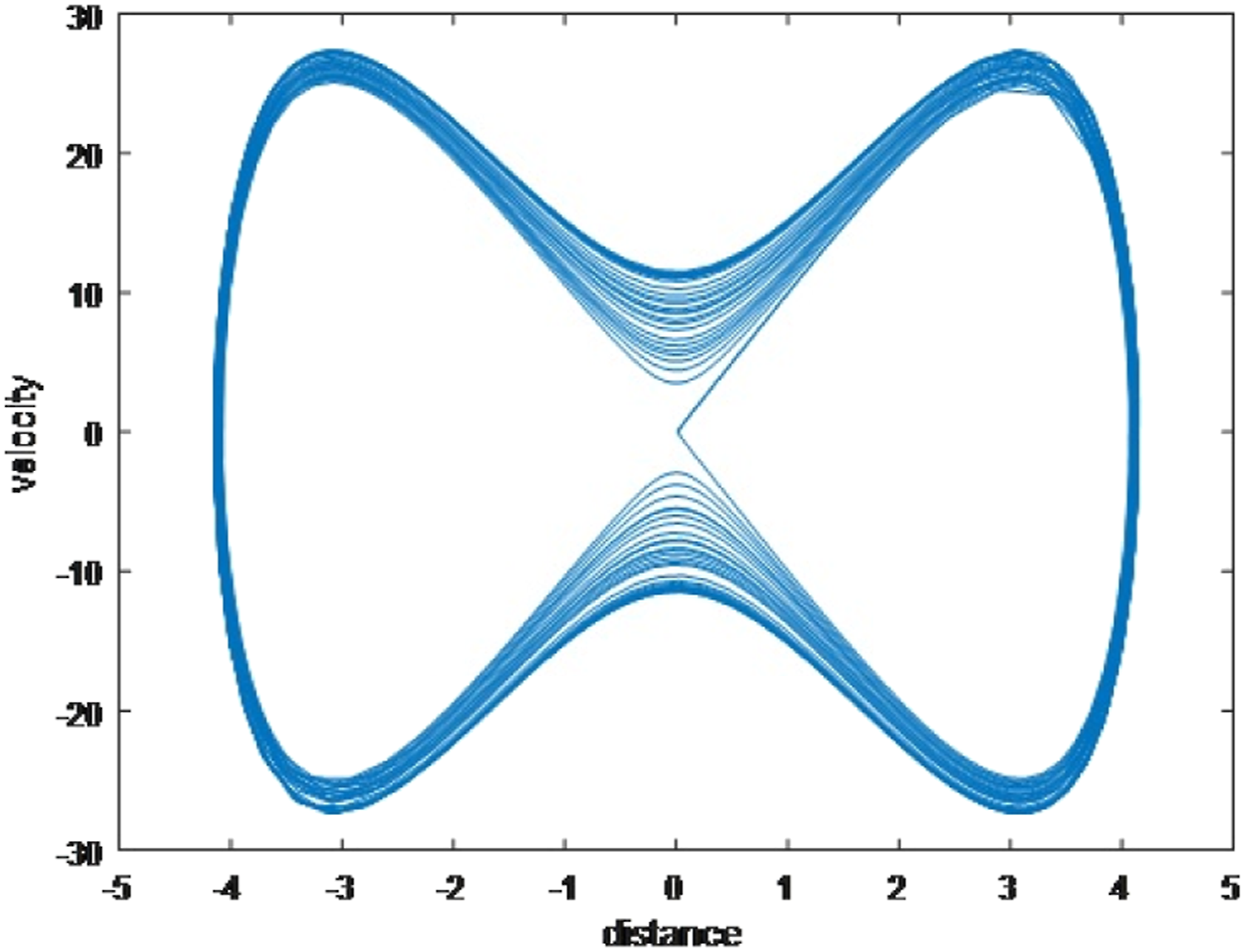
We see if the value of A is not close enough to one, it goes to limit cycle of center fixed point, while the solution diverge when A value is close to one as explained in the following (Figures 19–21). Phase portrait for the nonlinear oscillator system (4.11) with A = 0.9. Phase portrait for the nonlinear oscillator system (4.11) with A = 0.999. Phase portrait for the nonlinear oscillator system (4.11) with A = 0.9999.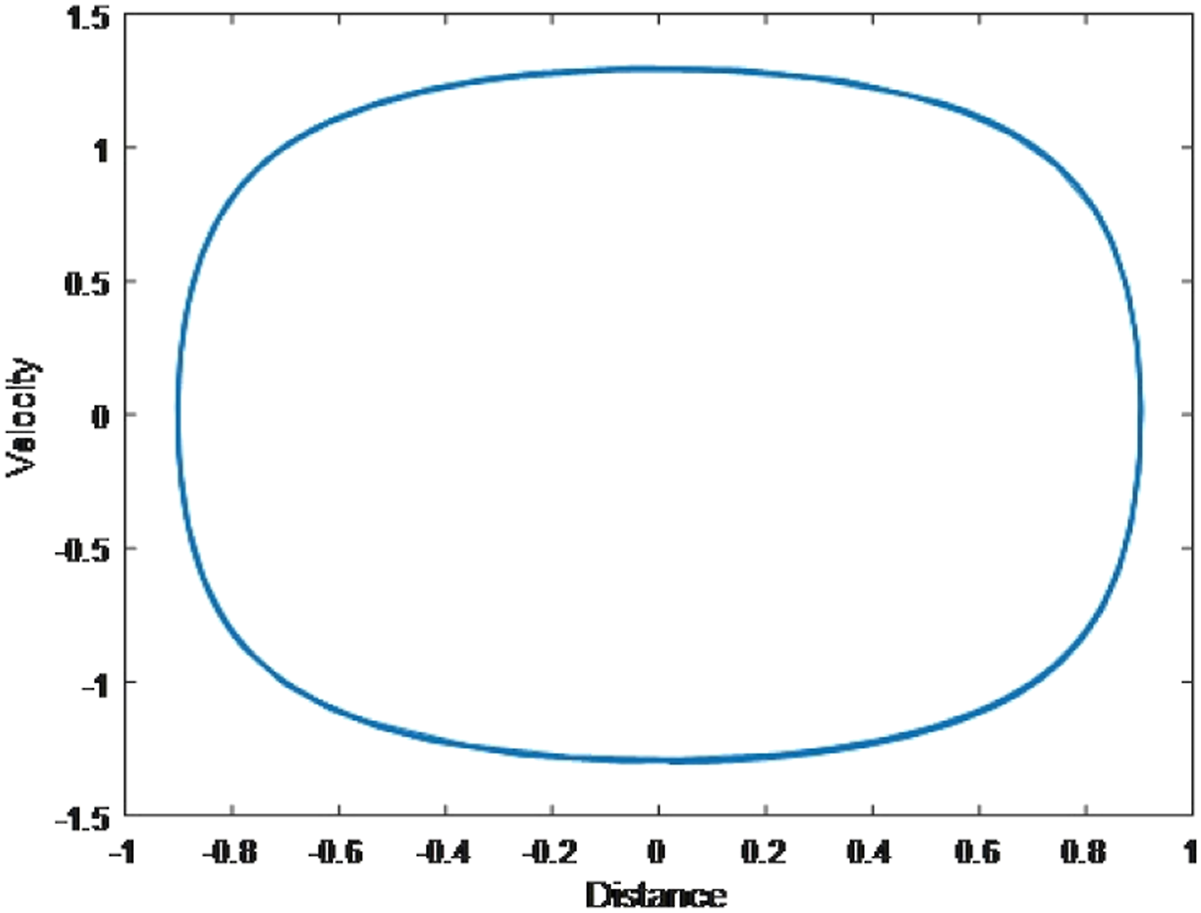
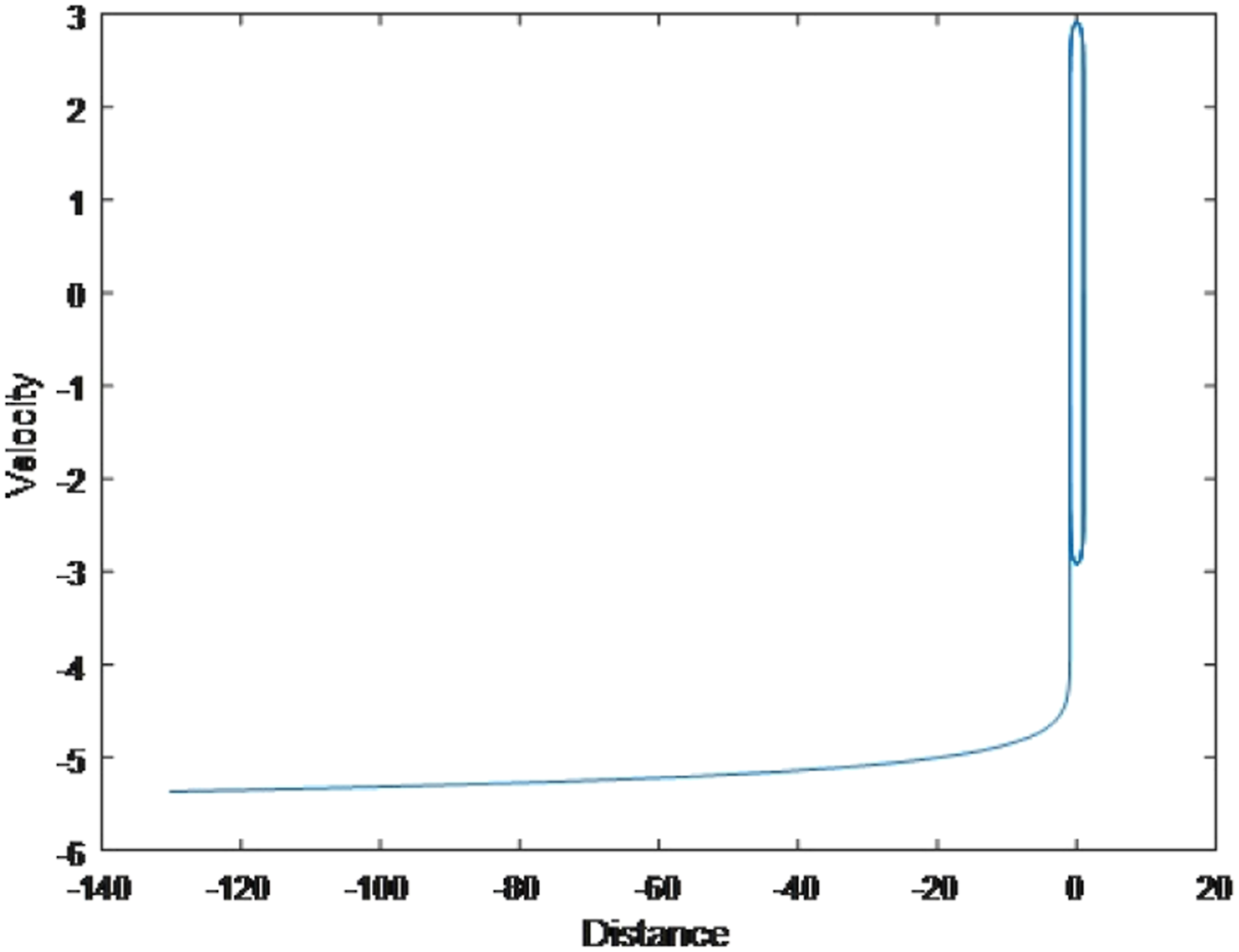
The solution will vanish when A = 1, it goes to infinity.
Results and discussion
The solution for equation (2.1) yields to frequency–amplitude relation Phase portrait for the nonlinear oscillator system (2.11) with A = 0.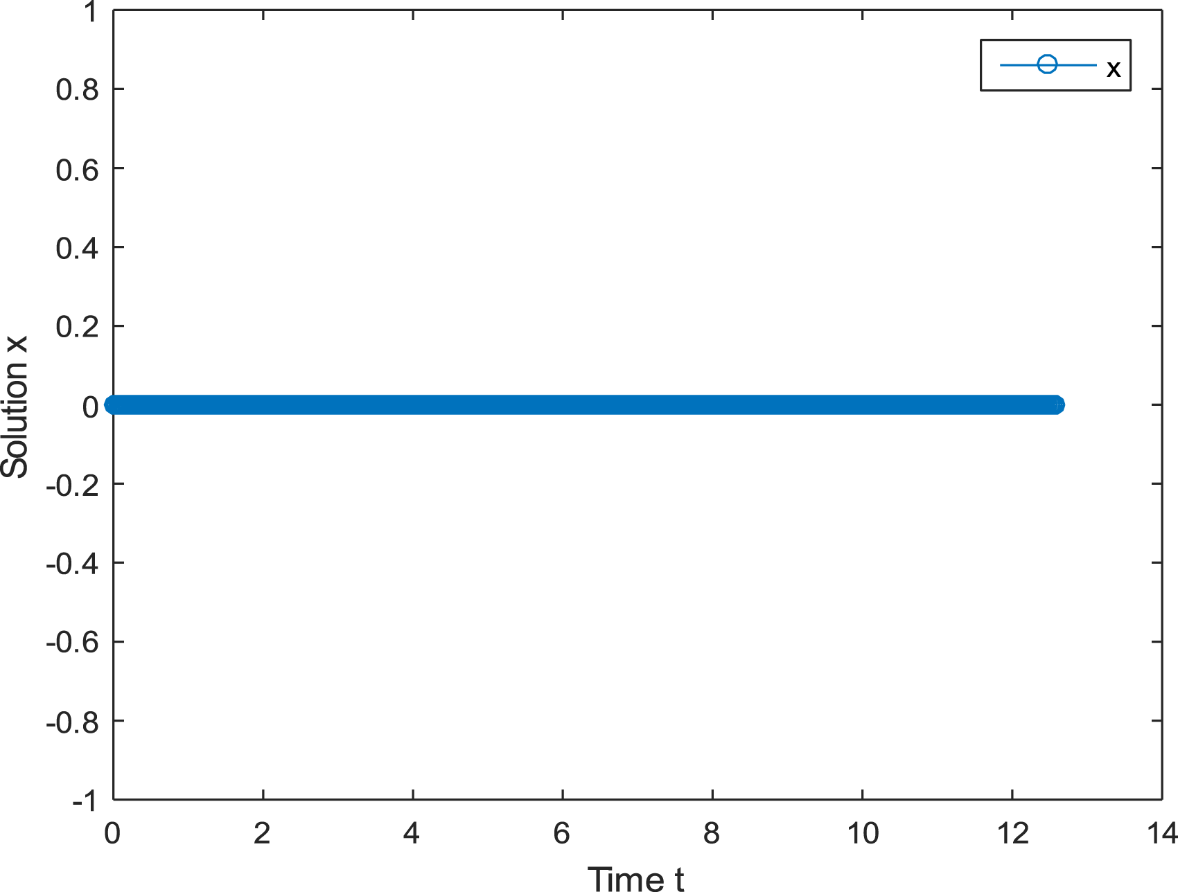
When A = 0.5, Phase portrait for the nonlinear oscillator system (2.11) with A = 0.5.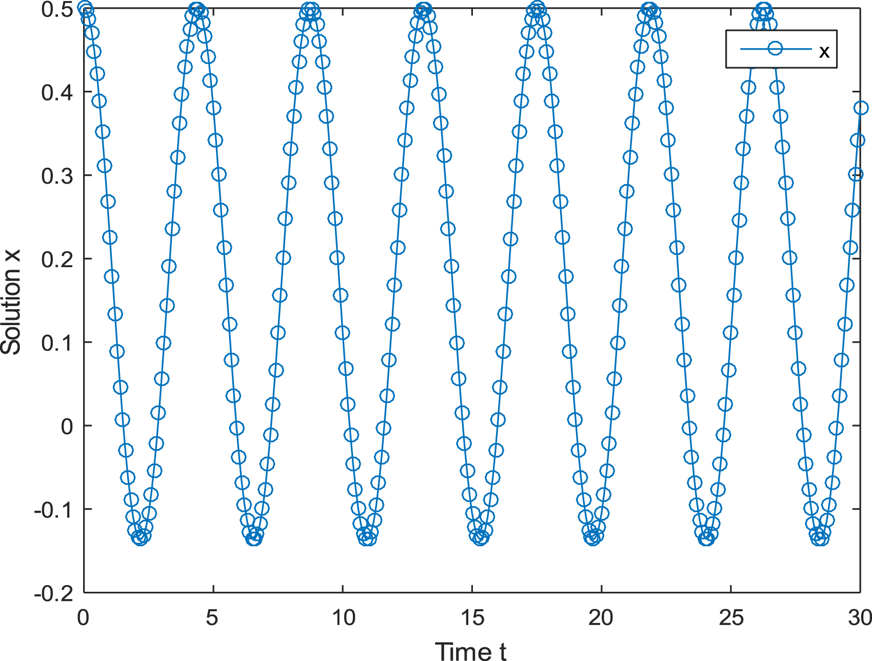
Now if we make the initial motion begin from A = 1, x(t)=1/3cos(3t)+2/3. From Figure 24, we can see this motion. Phase portrait for the nonlinear oscillator system (2.11) with A = 1.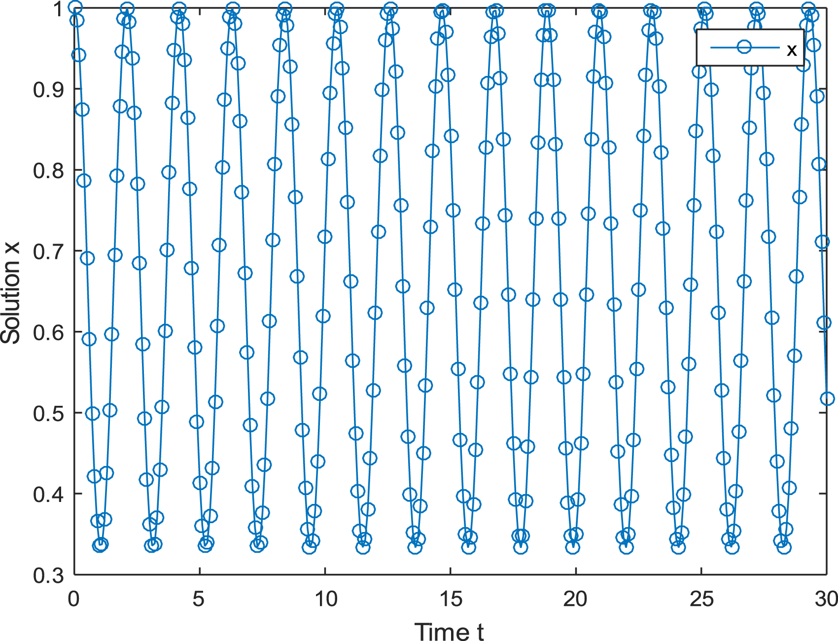
Finally, if we take A = 1.5, x(t) = Phase portrait for the nonlinear oscillator system (2.11) with A = 1.5.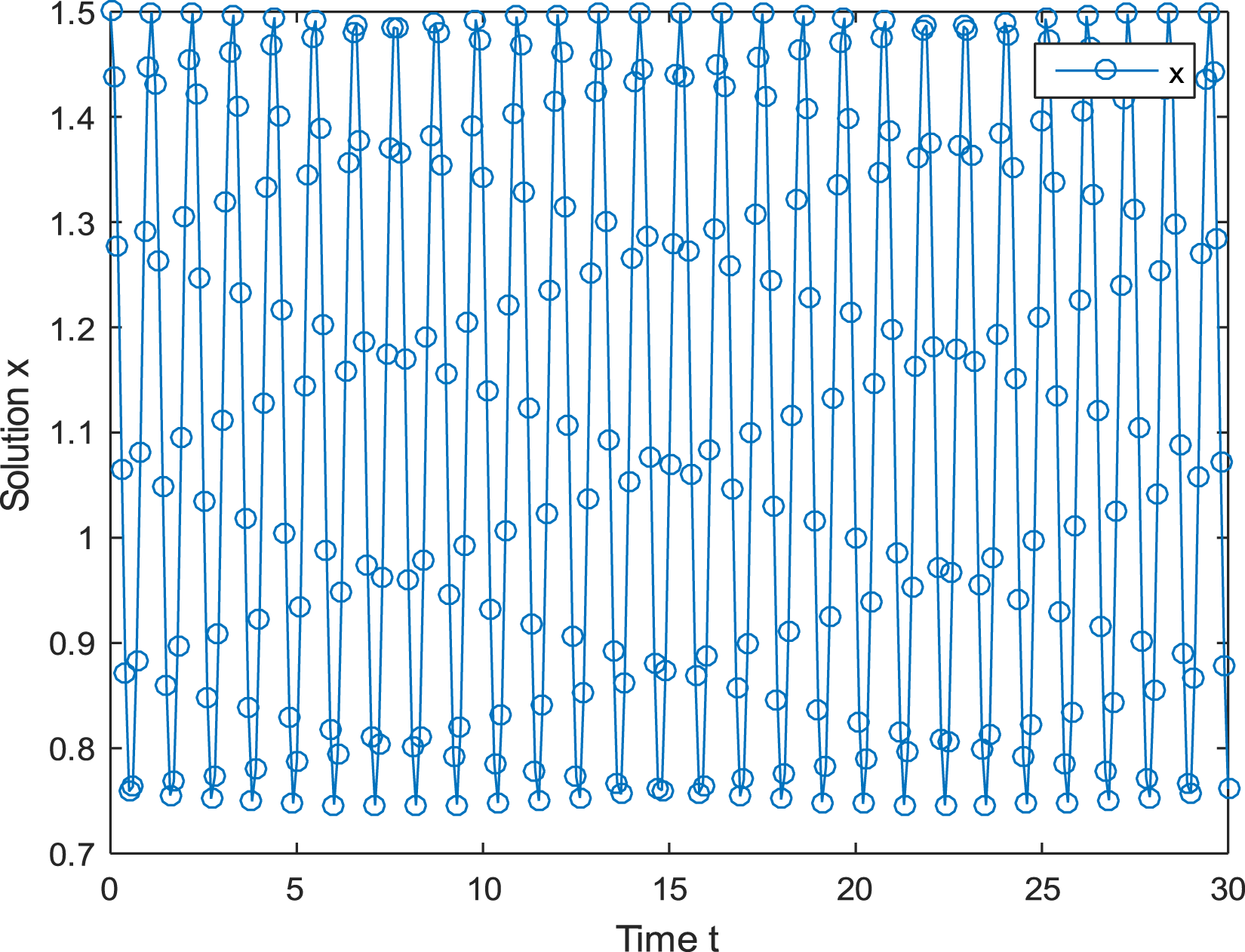
It is clear from (Figures 26–29) as value of A increases, oscillation increases, then the number of cycle also increases. Now we are going to consider the phase portrait which is the geometric representation of the trajectories of a dynamic system in the phase plane. So with α = 1, for equation (3.1), the dynamical system goes to a limit cycle from the fixed point (0,0), see Figure 26. Limit cycle when α = 1 for the system (3.2). Limit cycle when α = 10 for the system (3.2). Limit cycle when α = −20 for the system (3.2). Limit cycle when α = −100 for the system (3.2).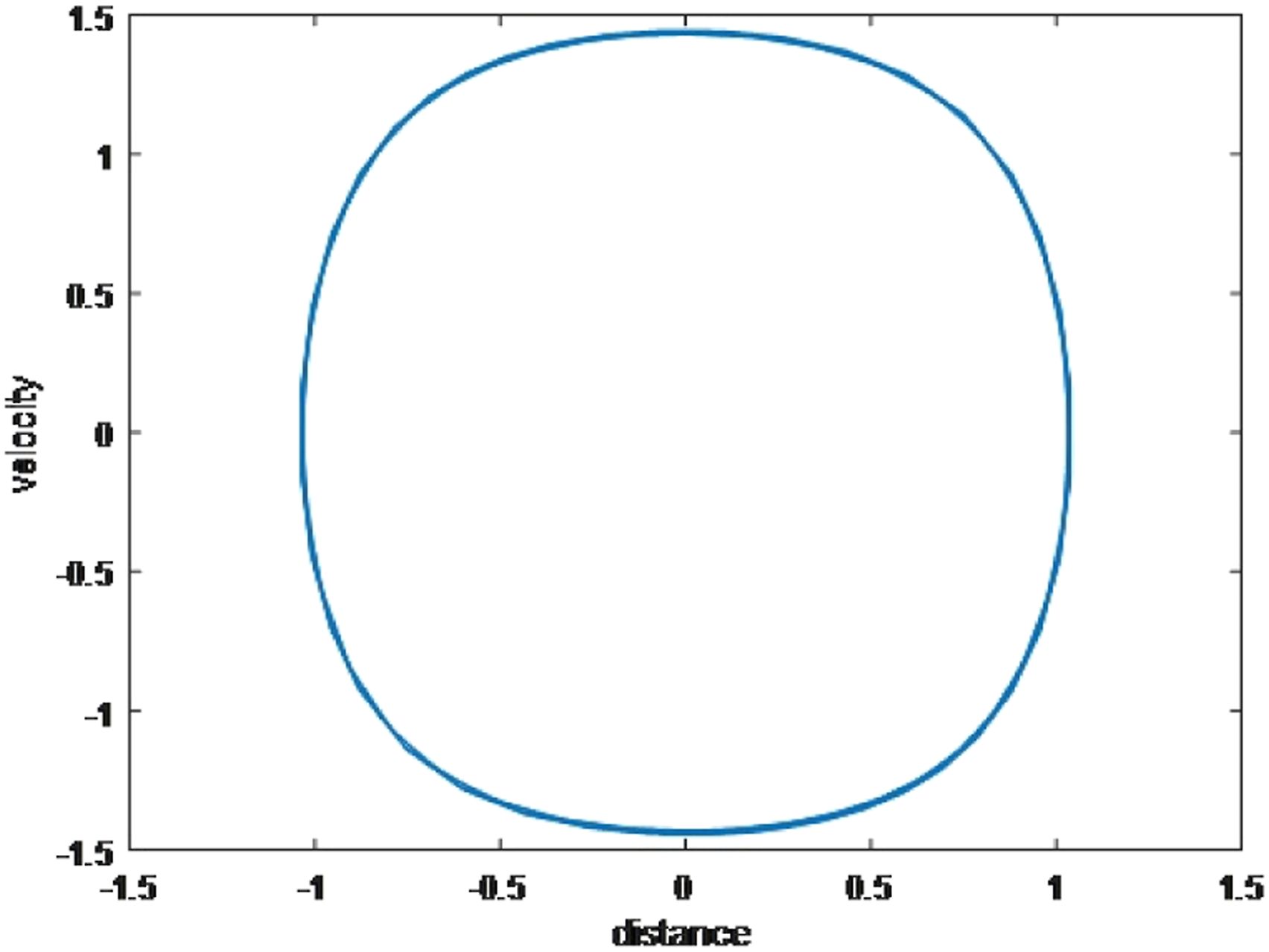
If the value of α increases positively, the shape of the spiral remains limited, as shown in The cycle’s shape remains limited even if alpha is increased for the largest positive, as seen in Figure 27.
When we take the negative values of α, we have two fixed points. The spiral limit cycle in two directions is shown in Figure 28.
Whereas increasing the negative values of α gives us clear picture about the movement of velocity and distance in the oscillator as shown Figure 29.
This work has many applications in different field such as physics Ref. 13 and financial market Ref. 14, and we can make this for many other applied areas that use oscillating behavior.
Conclusion
We get by power series a solution for a nonlinear oscillator differential equation that is depending on the analytical method, We solve a nonlinear oscillator differential equation based on the analytical method using a power series, whereas many other articles focus on guessing functions or an approximation one. Then we study the fixed points by converting the differential equation (2.1) to system of two non-linear differential equations studying their stability. Using Matlab code ode45, we get a graphical simulation for the behavior of the solution, moreover by multiplying the parameter α with linear term in equation (2.1) to study bifurcation, so we get two fixed points in oscillating movement with two limit cycle when α < 0. When we add more nonlinear terms, as in equation (4.3), the spiral movement increases the number of cycles as the value goes down. we find that the oscillator will diverge when we begin with value of A = ±1, and it goes to stable limit cycle when it is close to zero, we take more general nonlinear differential equation to study their fixed points and stability. Finally, we see that the power series solution gives us more accurate solution than other papers which study this type of equation. In this study, we see the frequency of the oscillator for the nonlinear equation that we get analytically meet the approximate values Refs. 9–41, where the analytical solution for infinitely many nonlinear term of this type of oscillator is given.
Footnotes
Acknowledgments
The authors thank Palestine Technical University- Kadoorie for their financial support and Jihad Asad would like to thank Dr. Nadia Hamad for proofreading and Language editing.
Declaration of conflicting interests
The author(s) declared no potential conflicts of interest with respect to the research, authorship, and/or publication of this article.
Funding
The author(s) received no financial support for the research, authorship, and/or publication of this article.