Analysis of separating acoustics from the thermoacoustic system of methane combustion based on Reynolds-averaged Navier-Stokes and linearized Navier-Stokes equations

Abstract

A model coupling Reynolds-averaged Navier-Stokes (RANS) method and linearized Navier-Stokes equations (LNSEs) was established in order to investigate the acoustic excitation and attenuation effect from a coupling perspective of time–space–frequency under various flow velocities and mass fractions of methane. Results show that the energy distribution of acoustic modes under high-frequency acoustic excitation is more uniform. The amplitude of the acoustic oscillation at a multiple coupling physical field is 10,000 times higher than that at simple flow field. The case when ${\mathrm{w}}_{\mathrm{C}\mathrm{H}4}$ = 0.8 owns the largest percentage of energy conversion from fundamental to high-frequency signals, the largest percentage of transmitted waves from the combustion chamber system to outside and the strongest non-linear effect. When ${\mathrm{w}}_{\mathrm{C}\mathrm{H}4}$ rises, the amplitude of oscillations at points and the attenuation effect of high-frequency signals along the axial are enhanced. At the case of U_in = 15 m/s, the amplitude of harmonics is reduced by 18% compared with other cases, while the proportion of the high-frequency harmonic increases, proving the non-linearity cannot be neglected in this case. As velocity rises, the energy conversion from fundamental to high-frequency signals enhances; while closer to the outlet position, the more complex the oscillation signal is. Model-shapes analysis shows that a case of ${\mathrm{w}}_{\mathrm{C}\mathrm{H}4}$ = 0.8 owns the largest amplitude of the second harmonic at downstream of the burner, while the amplitude of the harmonics rapidly increases at U_in = 15 m/s at the end of the burner, which further indicates that the energy conversion of low-frequency signals to high-frequency signals occurs mainly in the middle and downstream regions.

Introduction

Thermoacoustic instability (TI) in combustion systems has remained a challenging problem for industry for decades, since it can lead to excessive heat transfer loss, and can release the resonant oscillation pressure wave onto the combustors’ wall or jet panel of the engine, resulting in frequent loss of thermal integrity and structural integrity.^1,2 It usually caused by a non-linear interaction between non-stationary heat release and pressure fluctuations. ³ This interaction can cause large-amplitude periodic pressure oscillations, resulting in combustion problems ⁴ or even severe engine damage. Therefore, it is necessary to understand how the system responds to parameters. ⁵ In order to investigate the intrinsic mechanism of TI, many researchers have made a lot of efforts. ⁶

Numerical methods are widely used to explain and predict thermoacoustic oscillation in various combustion systems. It has been demonstrated in various combustors that large-eddy simulation (LES) can successfully predict the characteristic frequencies and oscillation amplitudes of the system. ³ Compressible and the Helmholtz solver were used to solve the turbulent flow and the acoustics simultaneously by Selle et al. ⁷ Results showed that both non-reactive and reactive flows experienced lateral patterns of instability. The unstable mode in the non-reactive flow is caused by the processing vortex core (PVC). While in the reactive flow, the instability is generated by thermoacoustic coupling. LES was applied to a realistic gas turbine combustion chamber configuration to investigate the evaluation of the terms in the acoustic energy equation and the identification of the mechanism driving the oscillation. ⁸ Sun et al. ⁹ used the LES method to explore the generation and mitigation mechanisms of self-excited pulsation oscillations in a methane-fueled swirl combustor with and without an exit nozzle. To overcome the high computational cost required for LES, non-stationary Reynolds-averaged Navier-Stokes (URANS) simulations are used to obtain results as close to LES as possible. The URANS are also proven to be effective in predicting the mode frequencies, mode shapes, and oscillation amplitudes in classical Rijke tubes and Rijke tubes. A two-dimensional (2D) numerical simulation method based on unsteady compressible Navier-Stokes equations was used by Li et al. to analyze the combustion instability in a bifurcated tube with a flare, and the results showed that the constructed model can accurately predict the system mode frequency, mode shape, and sound pressure level. ¹⁰ Forced flame simulations obtained by the LES method and RANS method were compared by Rofi et al., ¹¹ and results showed that the LES based approach correctly predicted both the pressure field and the unstable acoustic behavior of the test-rig, while the RANS-COMSOL® simulation successfully detected the instability patterns observed in the experimental tests. Thanks to its high computational accuracy and computational efficiency, the combination of RANS and Helmholtz solver is considered as a promising method for predicting thermoacoustic oscillations. However, the current methods of numerical analysis either analyze the coupling effect of the overall physical field^12–14 or decouple the flame dynamics or acoustic phenomena in the physical field alone,^15–17 and the numerical analysis of oscillations under the coupling effect between fluid dynamics, flame dynamics, and chemical reactions needs to be further explored. Meng et al. ¹⁸ proposed a method coupling the RANS and linearized Navier-Stokes equations (LNSEs), aiming at predicting the acoustic damping effects with real geometry and different bias flow velocities. Results showed that the flame dynamic, the hydrodynamic, and the acoustic phenomena all can be considered when using LNSEs. However, the effect of the heat source released by the chemical reaction on the acoustic damping effect needs to be further explored. Accordingly, the main purpose of this paper is to study the acoustic propagation damping effect under the influence of steady-state flow field and heat release by coupling chemical dynamics, RANS, and LNSEs.

The analysis of the effects of various factors on the system thermoacoustic can provide a theoretical basis for controlling the generation of oscillations. The main sources that can excite thermoacoustic instability are vortex oscillation^19–21 and entropy oscillation. Therefore, the factors which have influence on vortex and entropy production will eventually have a certain effect on thermoacoustic instability.^22–24 Consequently, fluid properties and chemical reaction kinetics become the two main factors that have a significant impact on thermoacoustic instability.^25–27 The properties of the inlet fluid have an important influence on the combustion instability, such as turbulence intensity, ²⁸ fluid dynamical vortex, ²⁹ and inlet velocity. ³⁰ Besides, equivalence ratio has also been proved to have a significant influence on combustion instability. Multi-bifurcation behaviors of staged swirl flames fueled with methane at atmospheric pressure were experimentally investigated by Wang et al. ³¹ by varying the global equivalence ratios. Based on the characteristics of measured pressure oscillations and the associated results of phase space reconstruction, recurrence plots, and time–frequency analysis, they identified the multi-bifurcation behaviors of the thermoacoustic system with four different stability regimes. The vortical structures, dynamics, and interaction with a turbulent premixed flame in swirl-stabilized combustor under various equivalence ratios had also been investigated.^32,33 A large number of detailed studies have been conducted on the aspect of the effect of various factors on thermoacoustic instability, yet there are still gaps that can be further explored, such as the transmission, reflection, and transmission characteristics of acoustic waves under the coupling influence of fluid-thermodynamics from a perspective of time–space–frequency domain integrated analysis.

In conclusion, although a lot of studies have been done to break through the generation mechanism of thermoacoustic instability,^34,35 there are still possibilities for further analysis in numerical analysis, such as replacing the Helmholtz solver with LNSEs in order to obtain the coupling effect of flow field and the heat source from the chemical reaction on acoustic oscillations. In addition, it is also interesting to decouple acoustic from thermoacoustic systems and analyze transmission and attenuation characteristics of it from a multiple time–space–frequency perspective with the effect of various factors. Accordingly, the main objective of this study is to establish a model coupling RANS and LNSEs; the mean variation characteristics of the flow field are obtained by RANS and input as excitation into the LNSEs so as to gain acoustic oscillations. In addition, the heat source released by chemical reactions is also applied to the LNSEs as another excitation. The acoustic excitation and attenuation effect from a coupling perspective of time–space–frequency under various flow rates and mass fractions are further investigated. Furthermore, the reflective and transmissive effect of acoustic waves due to the difference in gas compositions and temperatures between the combustion system and the outside is rarely considered, which will also be explored in this paper.

Physical models and numerical methods

Boundary conditions

The cylindrical combustion chamber is 170 cm in length and 50 cm in diameter, as shown in Figure 1. Natural gas is injected into the chamber through a pipe aligned with the center line of the chamber. Before performing the model verification, the boundaries of the model are set accordingly to the experimental conditions. The fuel flow is 0.0125 kg/s, and the inlet temperature is 313.15 K. The corresponding air flow rate is 0.186 kg/s with the inlet temperature of 323.15 K. Fuel enters the chamber through a cylindrical air duct with a diameter of 6 cm, while air enters the chamber through a central annular air duct with a spacing of 2 cm. The fuel and air flow rates were 7.76 m/s and 36.29 m/s, respectively. The inlet air is composed of oxygen (mole fraction 23%), nitrogen (mole fraction 76%), and water vapor (mole fraction 1%), while the fuel is composed of methane (mole fraction 90%) and nitrogen (10%). Besides, all walls are set to adiabatic conditions. The pressure outlet boundary condition with a total pressure of 101,325 Pa is applied at the combustor outlet.

Figure 1.

Cylindrical combustion chamber.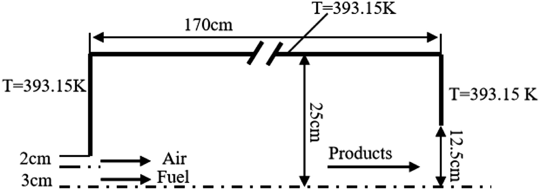

Governing equations

In this paper, a multi-physical field coupling model was built based on COMSOL software to simulate the combustion process of methane. The model is shown in Figure 2. The overall model is divided into four parts, namely, the k-ε model, the fluid heat transfer model, the concentrated matter transfer model, and the LNSEs for solving the acoustic wave equation. The former three models are coupled by the non-isothermal flow and the reaction flow multi-physical field coupling model, which can describe the mass and heat transfer phenomenon in the methane combustion process. RANS method is used to solve the mass, momentum, energy, and species transport equations in compressible fluids. Governing equations are given in equations (1)–(4):

Figure 2.

Multi-physical field coupling model.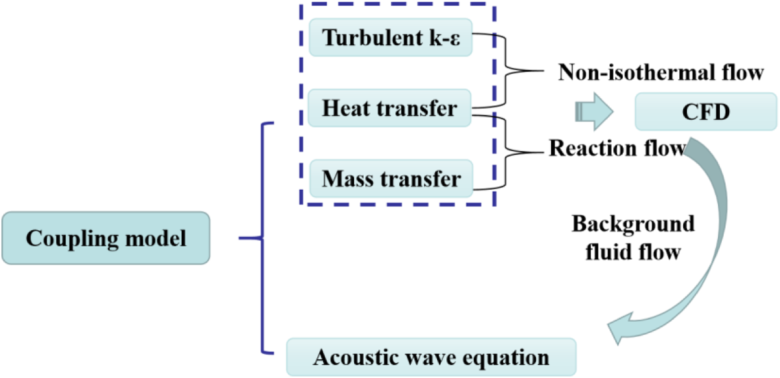

Mass conservation:

$\frac{\partial \rho }{\partial t}+\nabla \left(\rho \mathit{v}\right)=0$

(1)

Momentum conservation:

$\frac{\partial }{\partial t}\left(\rho \mathit{v}\right)+\nabla \left(\rho \mathit{v}\mathit{v}\right)=-\nabla \rho +\nabla \bullet \left(\overline{\overline{\tau }}-{\tau }_{ij}^{\prime }\right)$

(2)

Energy conservation:

$\frac{\partial }{\partial t}\left(\rho \mathit{E}\right)+\nabla \left(\mathit{v}\left(\rho E+\rho \right)\right)=\nabla \bullet \left(k_{eff}\nabla T-{\sum }_j{h}_{\xi }{\mathit{J}}_{\xi }+{\tau }_{eff}\mathit{v}\right)+S_h$

(3)

Species conservation:

$\frac{\partial }{\partial t}\left(\rho Y_i\right)+\nabla \left(\rho \mathit{v}{Y}_i\right)=-\nabla {\mathit{J}}_i+{\omega }_{\zeta }$

(4)

Thermodynamic state equation:

$\mathrm{\rho }=\frac{\mathrm{p}}{\left({\mathrm{R}}_{\mathrm{g}}/{\mathrm{M}}_{\mathrm{w}}\right)\mathrm{T}}$

(5)where $\rho$ represents density, v is velocity vector, t stands for time, p is pressure, T represents temperature, τ is the stress tensor, ${\tau }_{ij}^{\prime }$ is Reynolds stress tensor, ${\tau }_{eff}$ stands for effective stress tensor, E represents the total energy, $k_{eff}$ is conductivity, $h_{\xi }$ represents the entropy of species $\zeta$ , ${\mathit{J}}_{\xi }$ stands for the diffusion flux of species $\zeta$ , S _h means the fluid entropy source, R _g means the gas constant, M _w represents the molecular weight, and Y _i and ω _i mean the mass fraction and net rate of the production of species i.

After the flow field results of methane combustion are calculated, physical quantities such as temperature, pressure, and density in the computational fluid dynamics (CFD) model are mapped to the sound field through the background fluid flow coupling model for acoustic analysis and solution. The boundary conditions of each model are set based on the initial conditions set in the experiment. The two-step combustion reaction of methane is selected in this model, as shown in equations (6) and (7).

$2{CH}_4+3O_2=2CO+4H_{2}O$

(6)

$2CO+O_2=2CO$

(7)

Meshing

The simplicity of structured grids in application development, computation, and management is its most outstanding advantage. Automatic connection information shows that configured meshes require the least amount of memory for a given network size, and correspondingly faster simulations. However, structured meshes are severely limited in practical engineering, especially when the geometry is complex and certain regions require high resolution. It is very important to construct a network structure consisting of a sufficiently large number of elements to ensure that the simulation is accurate in the shortest possible time. In this study, a predetermined physically controlled method of constructing the mesh was used to improve accuracy, and the physical field-based control technique can effectively reduce user-defined errors. Figure 3 demonstrates the created mesh structure of CFD domain and acoustic domain, and the mapping of elements between two structures was performed through the background flow of the multi-physics field.

Figure 3.

Schematic drawing of the cell meshing (a) meshing of fluid domains, (b)meshing of the acoustic domain, and (c) enlarged view of the circled part of (a).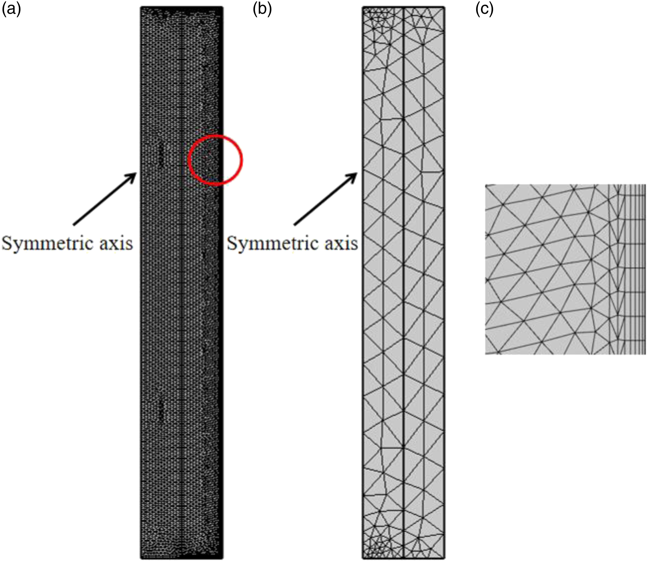

Turbulence model and chemical reaction validations and independence study

Model validations

Based on the established model, the corresponding boundary conditions were set up to simulate the methane combustion process, and the simulation results were compared with the experimental results to ensure the applicability of the model. The comparison between the simulated results distributed along the central axis of the burner and the experimental data can be observed in Figure 4. Meanwhile, the error ( $\mathrm{\chi }$ ) between the experimental and simulated data was plotted in the graph as a form of a bar chart. It can be viewed from Figure 4(a) that the simulated results are slightly higher than the experimental ones at the position close to the fuel inlet. However, the temperatures obtained by simulation fit well with the experimental ones obtained from Ref. 36 while at the location far from the fuel inlet. In general, the error between simulated one with experimental one is within 0.1, which can reflect the usability of the model. The comparison between the simulated mass fraction and the experimental data was made in Figure 4(b). It can be seen that simulated methane fractions were slightly lower than the experimental data at the position near the fuel inlet, while the fitting effect is better at the position far away from the fuel inlet. The selection of a more complex mechanism will make the results more accurate; however, it will lead to a surge in the calculation amount of the whole model at the same time. The deviation between the results of the simplified mechanism selected in this paper and the experimental results is within an acceptable range, so the model can simulate the methane combustion process well. The acoustic analysis in this paper is calculated based on the physical quantities such as temperature, pressure, and density mapped by the CFD model of methane combustion. The calibrated CFD model guarantees the accuracy of the acoustic analysis.

Figure 4.

Comparison between simulation results and experimental data.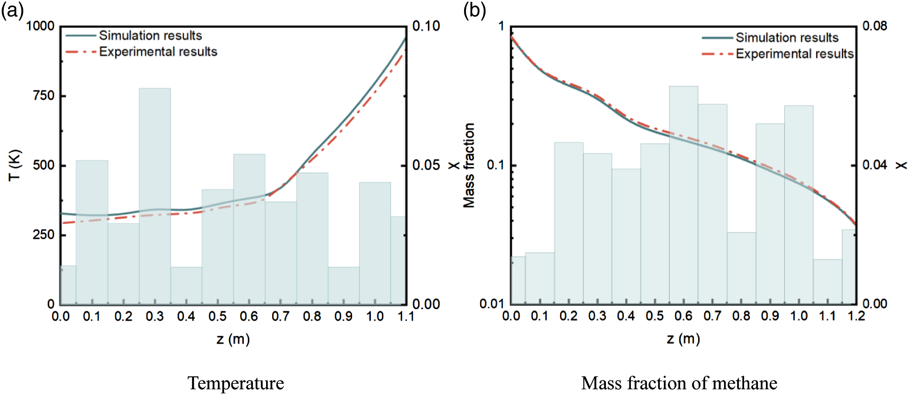

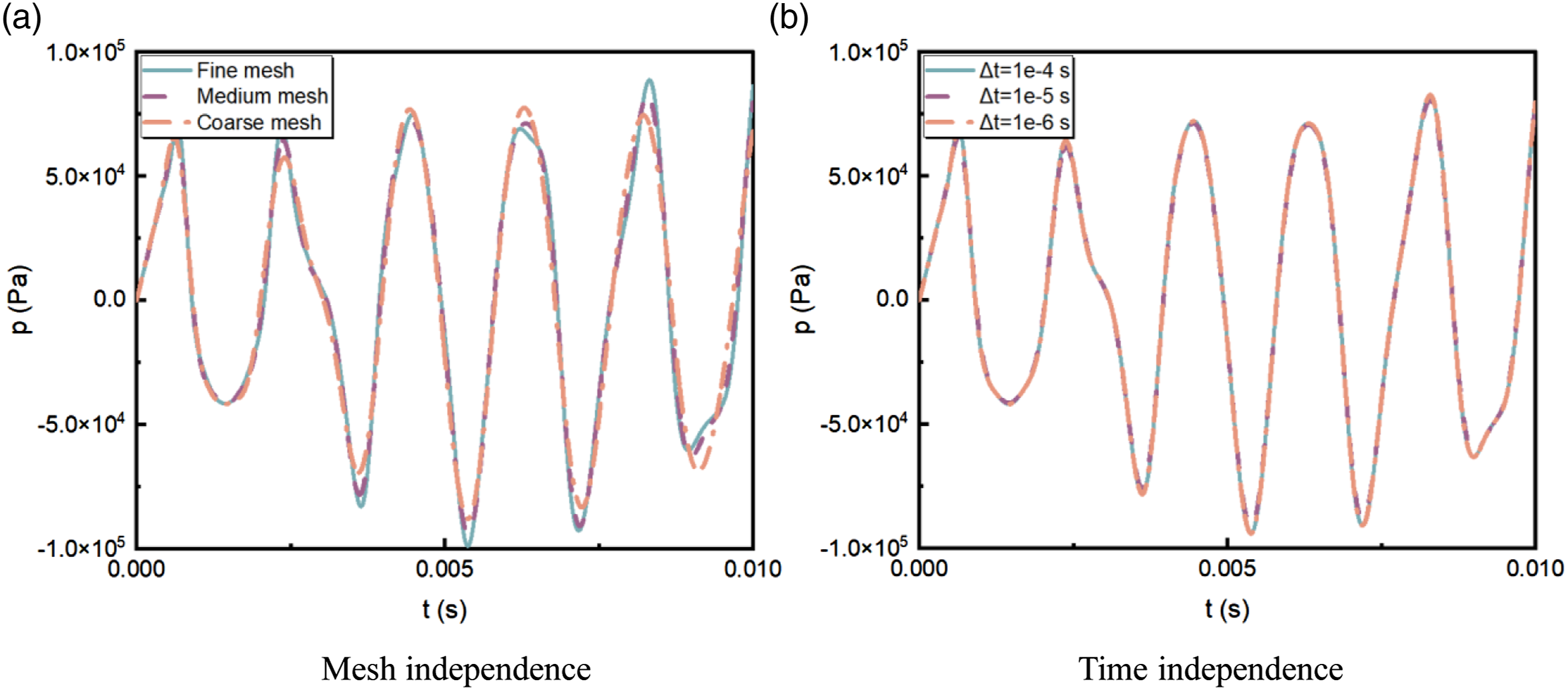
Time-independence and mesh independence

To ensure that the results of the numerical simulations at acoustic domain are grid-independent, a grid-independence test is required. ¹⁴ Three different mesh resolutions were generated in order to perform the mesh independence test. The fine mesh had about 2102 elements and was coarsened twice to produce a medium mesh and a coarse mesh with 820 and 454 elements, respectively. A comparison of the simulation results obtained from the three mesh resolutions is shown in Figure 5(a), which shows that the results obtained from the three resolutions do not differ much and the variation trend is basically the same. Considering the accuracy and computational cost, medium meshing was chosen for the subsequent simulations. Apart from the grid-independence test, a time-independence test is required to ensure that the results are independent of the time step. Simulation was conducted with three time steps, including 1e-4 s, 1e-5 s, and 1e-6 s. Figure 5(b) shows the variation of the amplitudes of acoustic oscillations at three time steps. It can be examined that various time steps have little effect on the change of amplitude, so a medium time step is chosen for the subsequent acoustic analysis in this paper.

Figure 5.

Variation of the amplitudes of acoustic oscillations at different mesh resolutions and time steps. ³⁷

Discussion of simulation results

Cavity acoustic modal analysis (acoustic modal analysis)

The analysis of the inherent acoustic modes of the combustor cavity is of great significance to optimize the design of combustion strategy and to reduce unnecessary instability. Therefore, the pressure frequency domain model in COMSOL was selected to analyze the boundary mode of the cavity combustor, while the plane wave with frequency varying from 0 to 1000 Hz is set as sound source, aiming to find the inherent acoustic mode of the cavity combustor.

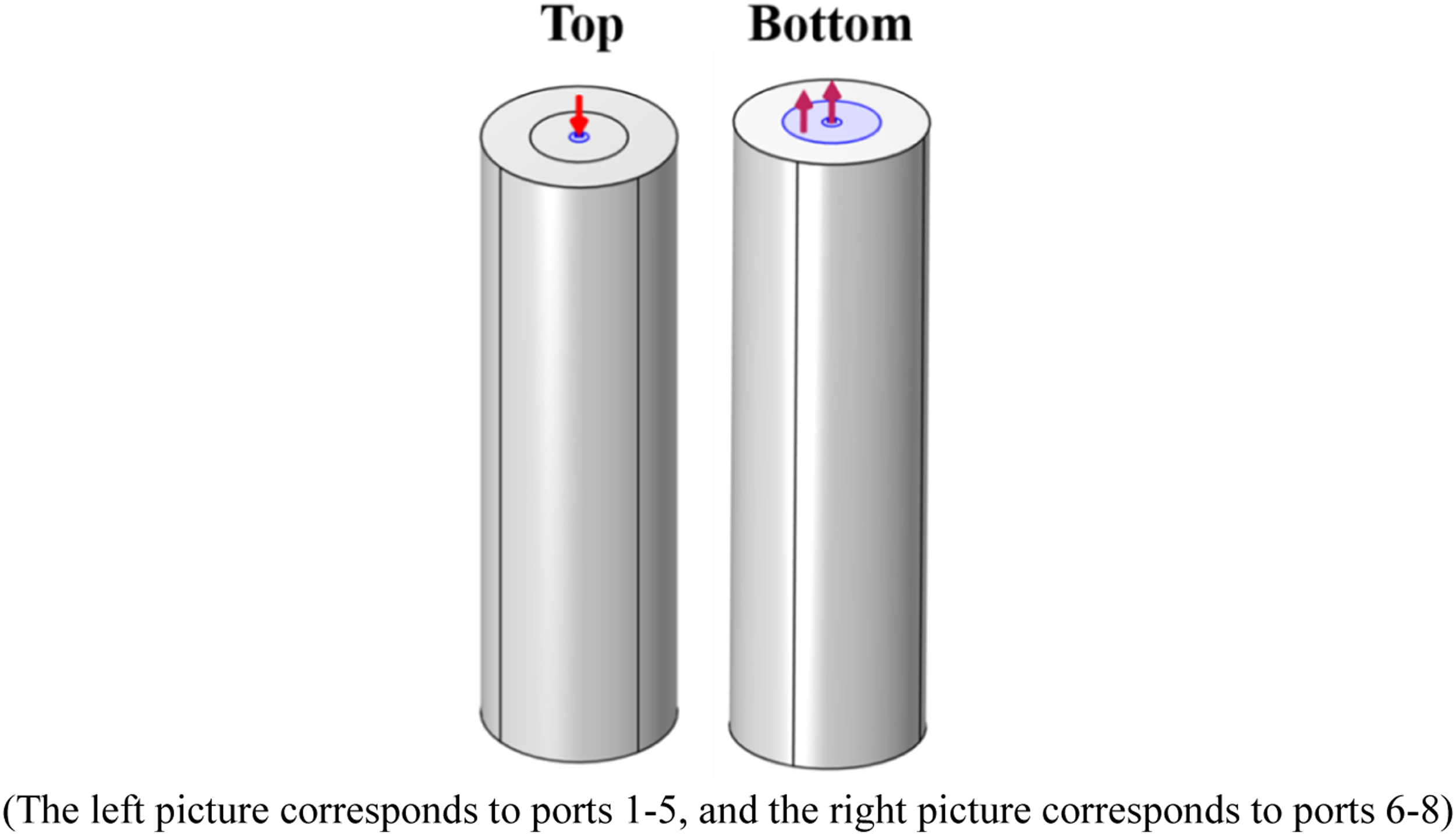
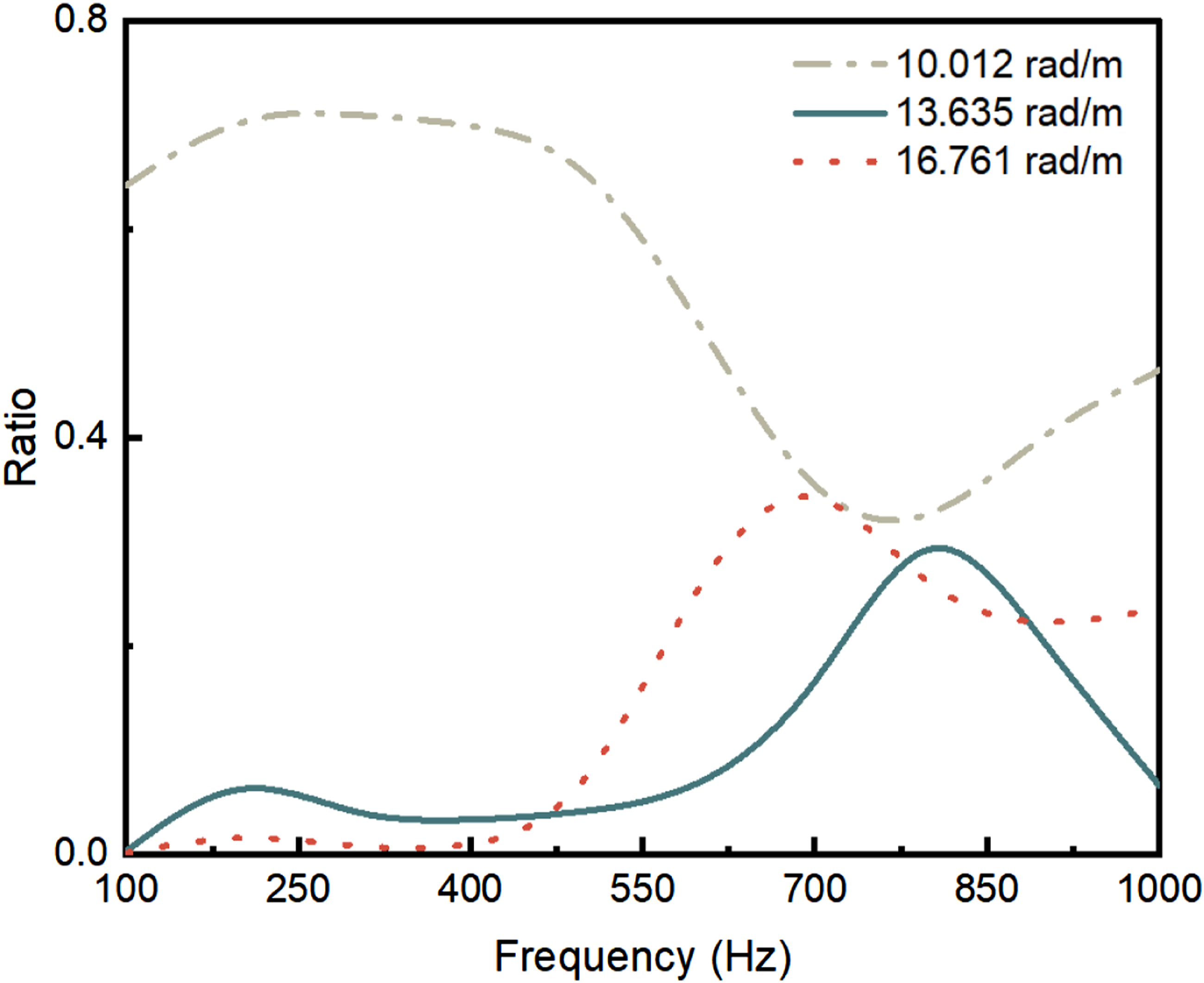
As shown in Figure 6, the cavity combustor mainly has three acoustic modes within 1000 Hz, and the corresponding out-of-plane wave numbers are 10.012 rad/m, 13.635 rad/m, and 16.761 rad/m, respectively. Port analysis was adopted to gain the amplitude of waves at the outlet position as well as the waves reflected back at the inlet, aiming to emphasize the contribution of each frequency waves. The specific settings of port analysis are as follows: a plan wave with an amplitude of 1 Pa was set at port 1 as acoustic excitation, the corresponding plane wave was absorbed by port 2, port 3–5 absorbed the reflected sound wave of three modes, while port 6–8 absorbed the waves of three modes transmitted to the outlet. The state of port 1 was on, while the state of other ports was off. The specific adding positions of the ports were shown in Figure 7. Based on port analysis and parametric scanning, the reflection and projection coefficients of each mode at different frequencies were obtained, and the proportions of each mode at different frequencies were further observed, as shown in Figure 8. As can be seen in Figure 8, proportion of the wave whose number equals to 10.012 rad/m is the largest at low frequencies, while the proportion of the other two modes increased gradually with increasing frequencies. When the frequency is close to 1000 Hz, the mode with a wave number of 10.012 rad/m is still the most important one. To sum up, it can also be concluded from Figure 8 that the modes and proportions of cavity acoustics gradually become particularly complex as frequency rises.

Figure 6.

Cavity acoustic modes.

Figure 7.

Port settings.

Figure 8.

Proportion of each mode at different frequencies.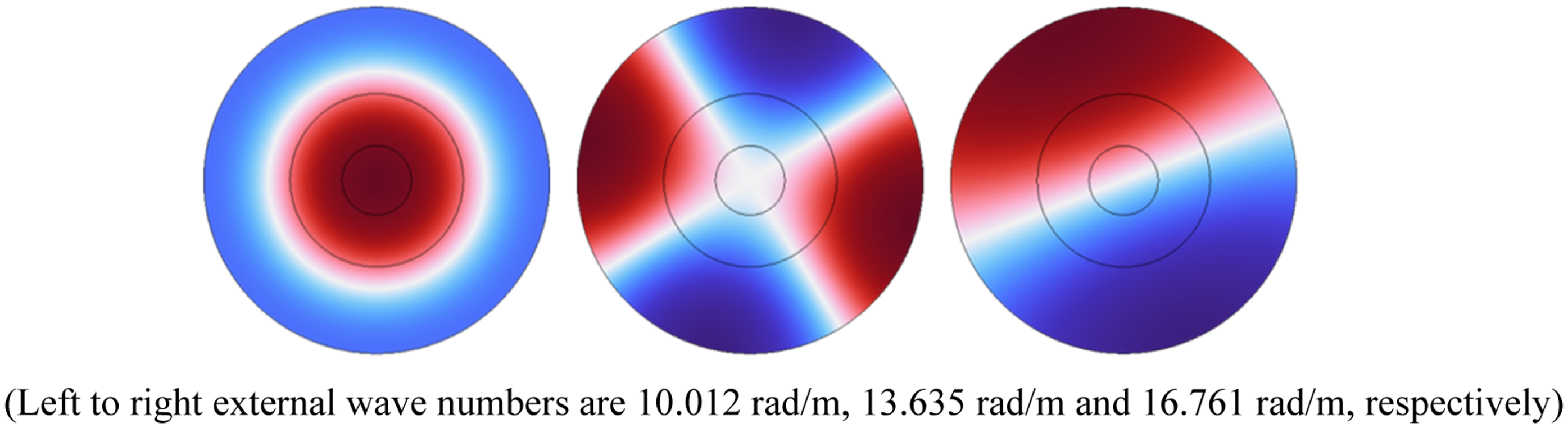

Flow-acoustic coupling analysis

Before analyzing the acoustic transmission characteristics during combustion, it is necessary to analyze the acoustic transmission under flow filed, clarifying the difference in sound pressure levels between the combustion and flow fields. The method of coupling flow field and sound field was adopted in this section to explore the acoustic transmission characteristics, and the plane wave was selected as the excitation to analyze the acoustic wave transmission under turbulence field.

Four monitoring points (P1–P4) along the central axis were selected to investigate the transmission characteristics of sound waves, which are away from the fuel inlet 1.7 m, 1.2 m, 0.9 m, and 0.4 m, respectively. The acoustic waves were analyzed from the perspectives of frequency domain and time domain, as shown in Figure 9. Figure 9(a) plots the root mean square (RMS) value of sound pressure at corresponding monitoring points under different frequencies. The main information that can be obtained from Figure 9(a) is that the further away from the fuel inlet the more likely it is to excite high-frequency acoustic oscillations, the maximum value of the amplitude of the sound pressure appears at point P4, and points P2 and P3 own more multiple peaks. Besides, the frequencies at where the waves gain their peaks gradually increases with rising distance away from the inlet, which further indicates that the low-frequency waves are dissipated in the propagation process. When putting sight on Figure 9(b), it can be obviously seen that the more intense the oscillation of the sound waves as the distance from the fuel entrance farther, which can be a further evidence of the attenuation of the of the low-frequency acoustic waves during transmission. In addition, the amplitude of waves at monitoring point P4 shows a trend of gradual increase, while at other monitoring points firstly increase and then decrease. Moreover, the amplitude of the sound pressure at P2 and P3 is significantly lower than other points by 30%, which is thought to be caused by the superposition of reflected sound waves.

Figure 9.

Acoustic characteristic analysis.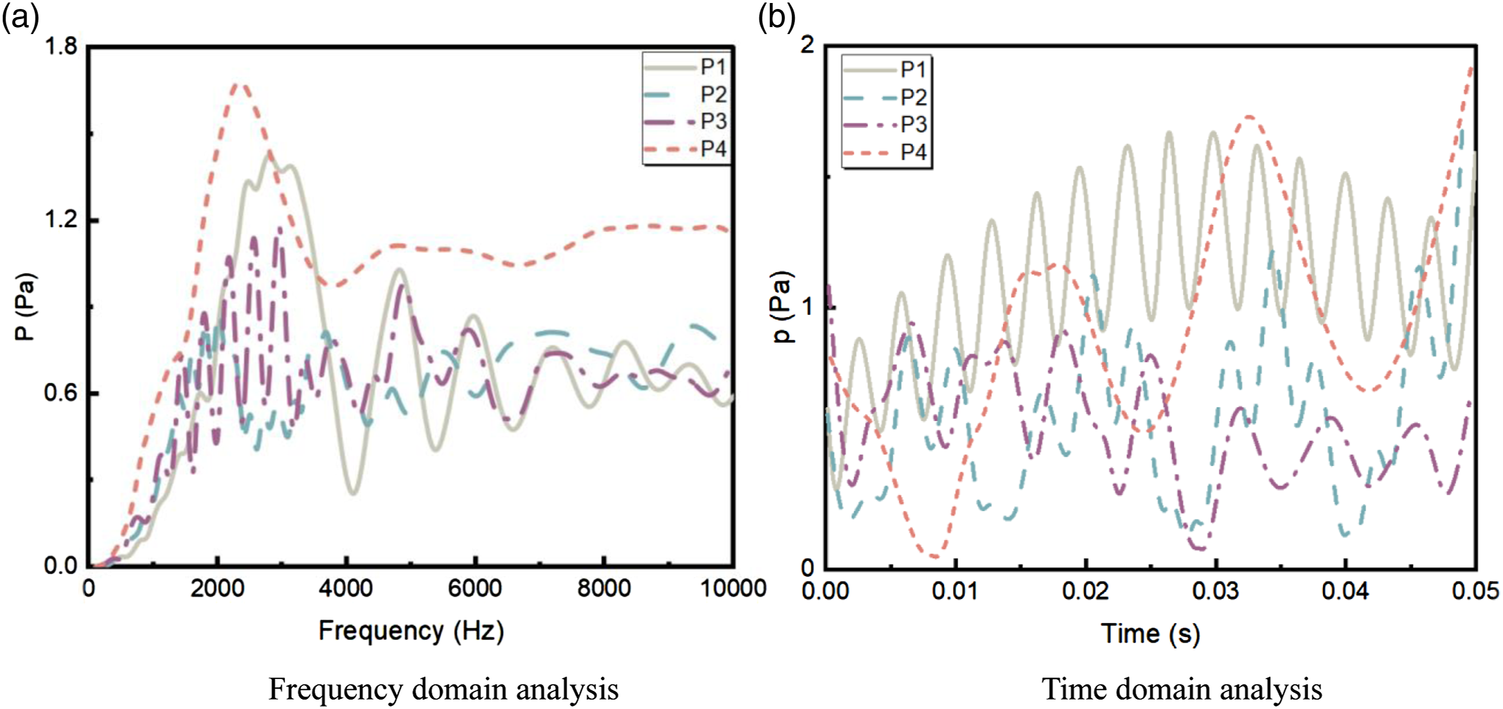

Thermo-fluid-chemical-acoustic coupling analysis

Based on the “non-isothermal flow,” “reaction flow,” and “background fluid flow coupling,” this section further analyzes the propagation characteristics of acoustic waves with a coupling effect of multiple physical fields. After literature review, it can be investigated that the factors such as fuel inlet velocities and equivalence ratios will disturb the waves in some ways. However, the quantitative relationship between the factors and acoustic attenuation is still unclear. Accordingly, the acoustic oscillation characteristics at monitoring points with different fuel mass fractions ( $w_{CH4}$ = 0.7, 0.8, and 0.9) and fuel inlet flow rates (U_in = 10 m/s, 20 m/s, and 30 m/s) were researched in this section. $w_{CH4}$ is defined as equation (8):

$w_{CH4}=\frac{m_{CH4}}{m_{CH4}+m_{air}}$

(8)where $m_{CH4}$ and $m_{air}$ represent the mass of methane and air, respectively.

From the perspective of time domain, the acoustic waves present a tendency of finite periodic oscillations at four points. At the beginning of the combustion, the amplitude of sound pressure at P4 gradually decreases while increases at other monitoring points. The amplitude of the sound pressure at P3 becomes the largest one as time goes by, which was thought to be caused by the superposition of the acoustic wave transmitted from P4 and the wave reflected through the outlet port. The amplitude of sound pressure at P2 is second only to P3, and the reason why the amplitude at P2 is smaller than that at P3 may be attributed to the attenuation in the process of sound wave transmission. As methane mass fraction increases, the amplitude at monitoring point P4 increases at the beginning, which is due to the larger heat source caused by the rising fuel mass fractions, resulting in a larger amplitude of the sound waves. Additionally, the difference between the amplitude of the sound waves at points P2 and P3 decreases with increasing methane mass fractions, and even coincides over a large area, which requires an analysis of the sound pressure characteristics at monitoring P1 to explain this phenomenon. As exit of the burner, monitoring point P1 is at the junction of combustion chamber and external; thus, the transmission and reflection of acoustic waves will occur at there. The amplitude of waves at point P1 in Figure 10 presents the portion of the sound pressure transmitted from the combustion system to the outside. The analysis of the acoustic waves at P1 at three operating conditions shows that the largest percentage of transmitted sound waves from the combustion chamber system to outside occurs at $w_{CH4}$ = 0.8, while the smallest one appears when mass fraction of methane is 0.7. Meanwhile, the amplitude of the reflected sound waves also shows the same trend that the minimum amplitude is at $w_{CH4}$ = 0.7 and the maximum amplitude is in a case of ${\mathrm{w}}_{\mathrm{C}\mathrm{H}4}$ = 0.8. The reason for the above phenomenon relies heavily on the sharp increase of the second peak at ${\mathrm{w}}_{\mathrm{C}\mathrm{H}4}$ = 0.8 at P4 in frequency domain analysis, as shown in Figure 11(b).

Figure 10.

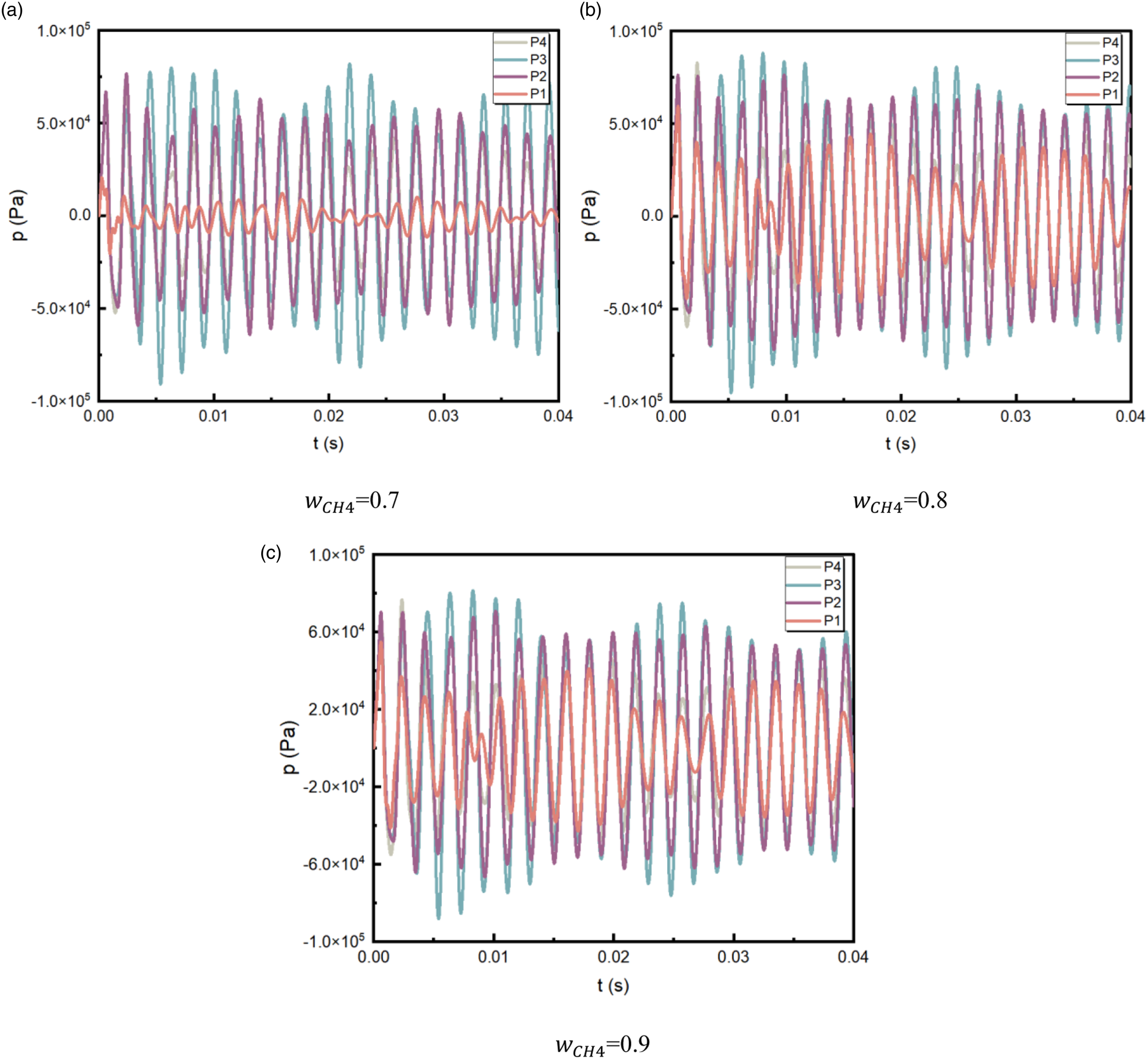
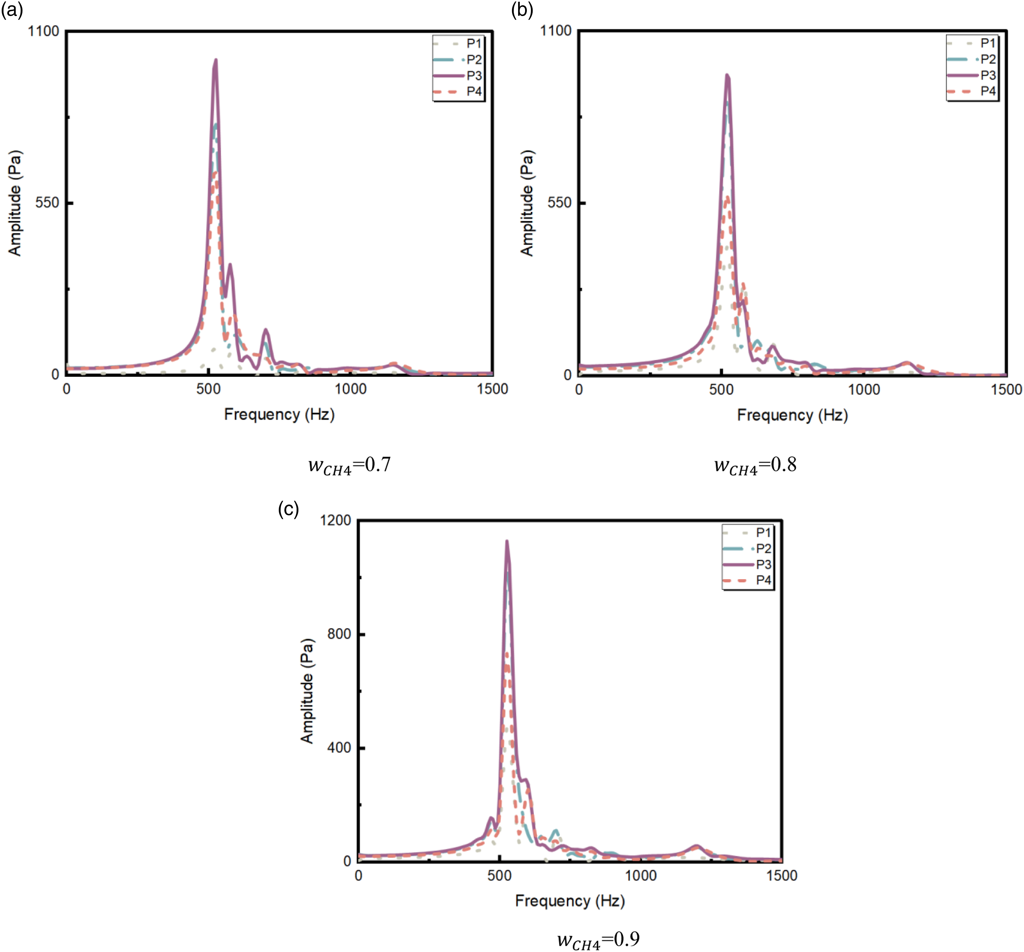
Time domain analysis at various $w_{CH4}$ .

Figure 11.

Frequency domain analysis at various $w_{CH4}$ .

The frequency domain structures of the RMS values of the acoustic pressure at monitoring points, which were mainly obtained by discrete Fourier transform of the sound pressure at time domain, were plotted in Figure 11. Overall, point P3 is the one with the largest peak value, which was caused by the superposition of waves generated by combustion and the emitted waves at the exit position, while the amplitude at P2 is smaller than P3 due to the attenuation effect of waves, and P1 owns the smallest amplitude. As shown in Figure 11(a), the first peak at monitoring point P3 appears near 500 Hz, the second peak is immediately adjacent to the first peak, the third peak appears near 700 Hz, and the frequency corresponding to the appearance of the first peak at the other monitoring points is the same as that at monitoring point P3, which is near 500 Hz, but the frequency corresponding to the second peak is larger than that at monitoring P3, while the third peak exists only at detection points P2 and P3. The appearance of the second and third peaks implies that the non-linear effects of the system are not negligible. P2 and P3 possess higher second peaks than others, saying that the non-linear effects in the transmission of acoustic waves are enhanced, in other words, energy transfer from fundamental wave to high-frequency acoustic waves during wave transmission gradually raise. As mass fraction of methane changes, maximum value of the second peak at P4 appears at $w_{CH4}$ = 0.8, suggesting that the non-linear effect is the largest at this case. The second peak of P3 and P2 nearly disappear with rising mass fractions of methane, denoting that the dissipation of high-frequency sound waves goes up at the same time.

In order to further investigate the attenuation characteristics of acoustic waves with different frequencies as time goes under various working conditions, the wavelet analysis-based time–frequency diagrams at P2 and P3 were plotted in Figure 12. From a general perspective, the energy of the acoustic waves is mainly concentrated at 500 Hz in the case of methane mass fractions equal to 0.7 or 0.9, while the energy of the acoustic waves gradually shifts to the high-frequency components (510 Hz and 700 Hz) at $w_{CH4}$ = 0.8. From the spatial point of view, in the process of acoustic wave transmission from P3 to P2 at all cases, it is obvious that the frequency component near the second harmonic (550 Hz) gradually decays, while the frequency component near the third harmonic (700 Hz) attenuates slightly less than at 550 Hz. From the point of view of temporal acoustic wave transmission, when $w_{CH4}$ = 0.8, waves of high-frequency (705 Hz) were excited with rising time, yet quickly dissipated, while the energy of the fundamental wave was briefly transferred to a slightly higher frequency (510 Hz) as time increases and then returns to its original state. To sum up, the non-linear effect of the system is the strongest and the share of the energy transferred from high-frequency to the low-frequency is the largest at $w_{CH4}$ = 0.8, clarifying the strongest acoustic absorption effect in this case.

Figure 12.

Time–frequency analysis at monitoring points P2 and P3: (a) 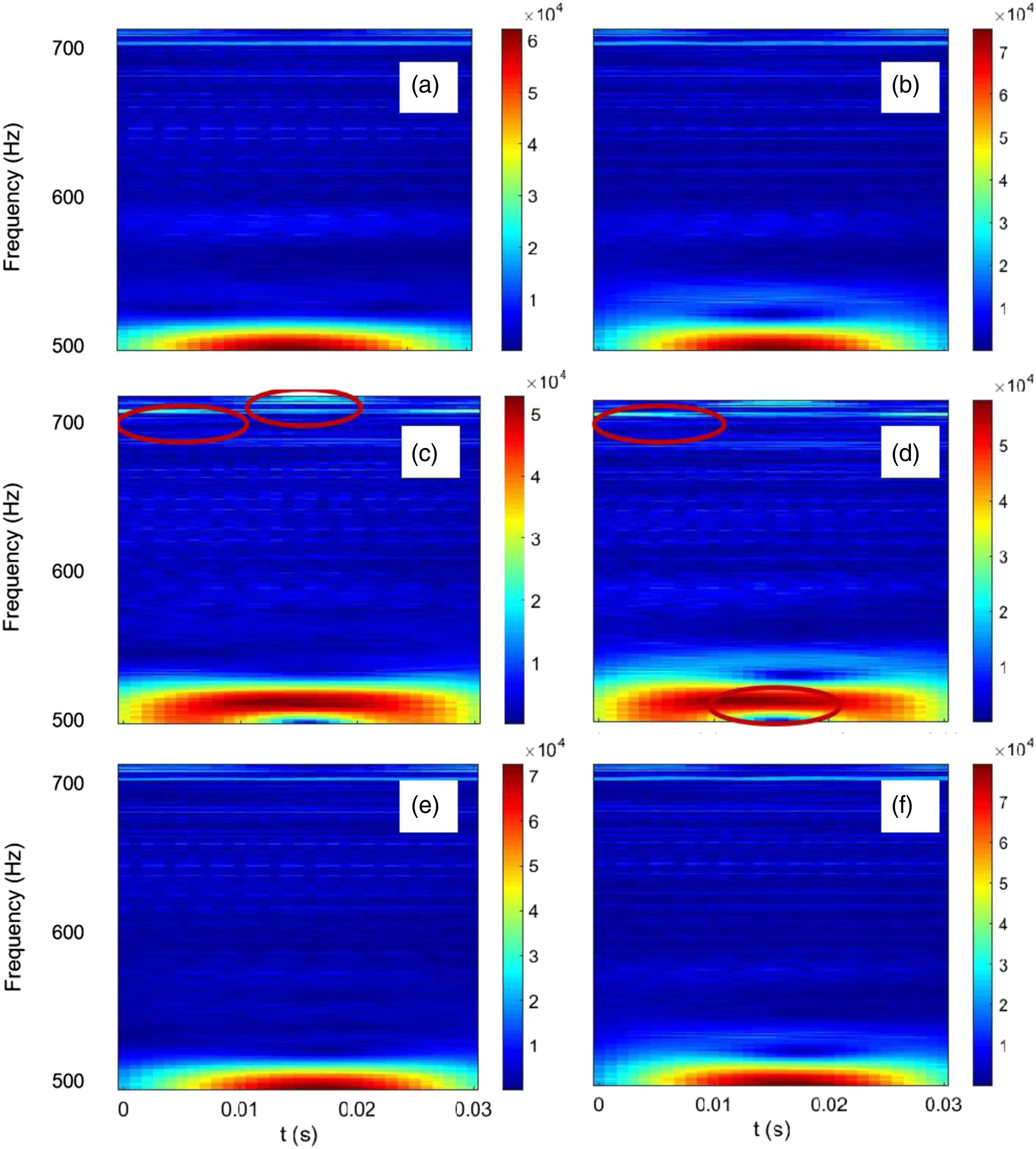$w_{CH4}$ = 0.7, at point P2, (b) ${\mathrm{w}}_{\mathrm{C}\mathrm{H}4}$ = 0.7, at point P3, (c) ${\mathrm{w}}_{\mathrm{C}\mathrm{H}4}$ = 0.8, at point P2, (d) ${\mathrm{w}}_{\mathrm{C}\mathrm{H}4}$ = 0.8, at point P3, (e) ${\mathrm{w}}_{\mathrm{C}\mathrm{H}4}$ = 0.9, at point P2, and (f) ${\mathrm{w}}_{\mathrm{C}\mathrm{H}4}$ = 0.9, at point P3.

According to previous analysis, mass fractions of methane have a certain impact on frequency domain and time domain characteristics of acoustic oscillations. The literature review also shows that the fuel inlet velocity also has an important impact on oscillations. Therefore, this section will discuss and analyze the influence of different inlet velocities (U_in is 10 m/s, 15 m/s, and 20 m/s, respectively) on sound pressure oscillations from time and frequency domains. Figure 13 displays time domain characteristics of sound pressure at four monitoring points under various flow velocities. It can be observed that the acoustic pressure oscillations show a periodicity trend at U_in = 10 m/s, while present a high degree of non-linearity when flow velocity increases. The amplitude of oscillations at P4 is smaller than at other points when the flow velocity is 10 m/s, which is thought to be caused by the acoustic reflection at the interface between the system and the outside, while it shows a dramatic increase with rising inlet flow rates, indicating that the non-linear effect of the system enhances with increasing velocities. The maximum amplitude of oscillations at P4 occurs at 0.013 s when U_in is 15 m/s, while it appears at 0.013 s at U_in = 20 m/s, which indicates that decay rate of the non-linear effect increases with rising flow velocity. For points P2 and P3, the amplitude of oscillations shows a gradual increase trend at a fuel flow velocity of 15 m/s or 20 m/s, attributing to the transmission of large-amplitude waves at P4. Regarding monitoring point P1, as the fuel velocity increases, ratio of the amplitude of sound wave at P1 to the amplitude of the sound waves at P4 increases, showing an increase in transmission coefficient of the sound wave between the combustion system and the outside. It is also worth noting that the amplitude of the sound pressure at monitoring point P2 is greater than that at P3 as the flow velocity increases, meaning that waves of higher amplitude may be excited during the forward and reflected transmission of acoustic waves.

Figure 13.

Time domain analysis.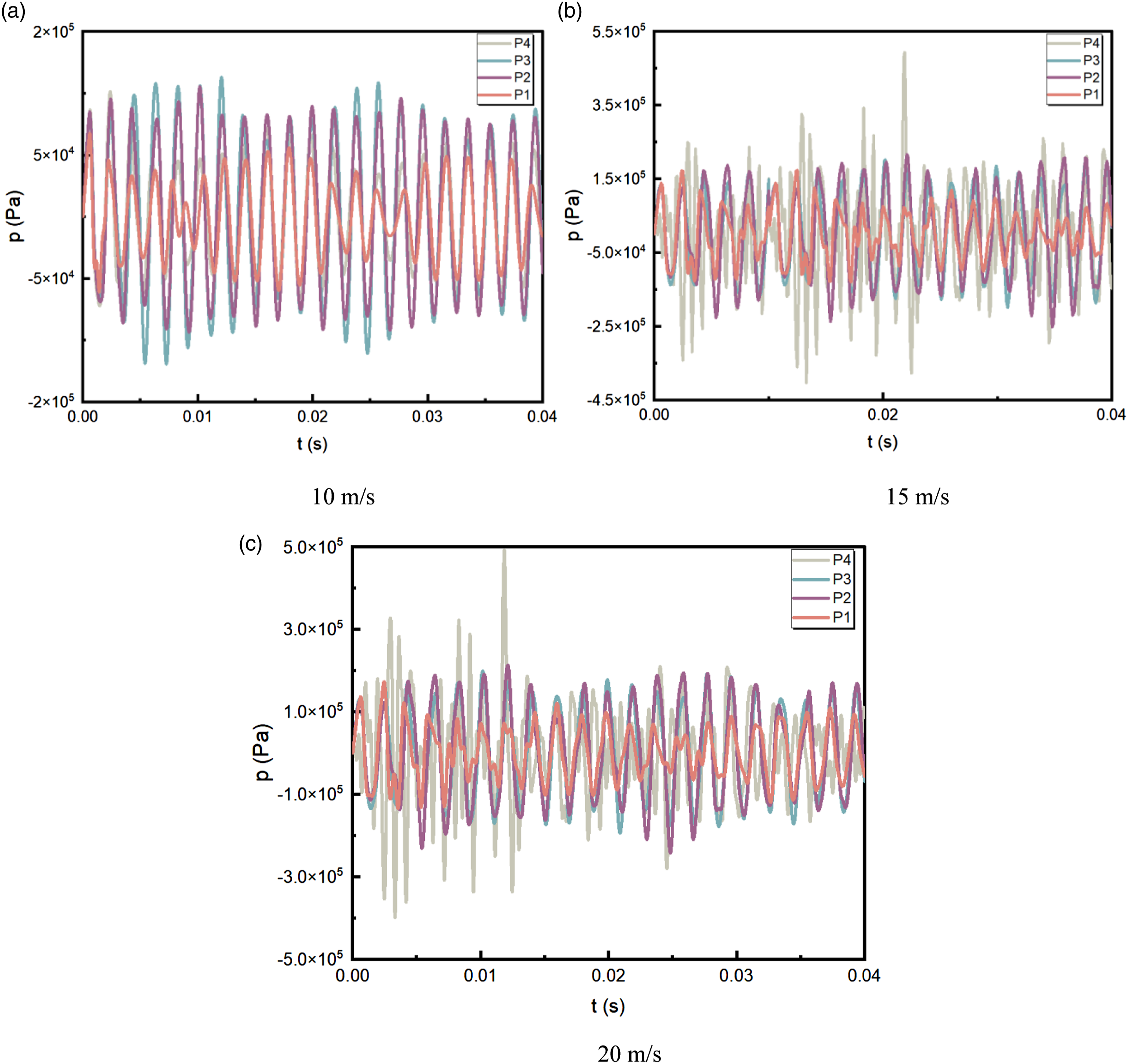

The discrete Fourier transform of the time domain signal was performed to obtain the frequency domain structure signal of the acoustic pressure various flow rates as shown in Figure 14. From Figure 14(a), it can be investigated that monitoring point P4 excites the fundamental wave (500 Hz) and the first harmonic (510 Hz), while the amplitude of harmonics at monitoring points P3 and P2 is higher than at P4 due to the superposition effect of forward transmission and emission of acoustic waves, and even excites the second harmonic of higher order, indicating that the non-linearity of the system is strengthened at this time with increasing distance, which further emphasizes the viscous dissipation effect of the system cannot be negligible. The amplitude of harmonics at a velocity of 15 m/s is reduced to 18% of at other cases, yet the proportion of the second harmonic increases, proving the non-linearity cannot be neglected in this case. High-frequency acoustic waves above 1000 Hz were excited during acoustic transmission process, which can be observed from structural characteristics of the frequency at P4. The coexistence pattern of multi-frequency signals at P4 is shown at Figure 14, indicating a strong energy transformation from fundamental wave to higher harmonics in this case. However, the high order harmonics quickly attenuated off in transmission process, which was concluded from there nearly no significant high-frequency harmonics at other monitoring points. When the flow rate increases to 20 m/s, the structure of the frequency components at four points becomes more complex. The analysis of the monitoring point P3 shows that the first harmonic, the second harmonic, and even the third harmonic (near 1150 Hz) are excited, indicating that the energy conversion from the fundamental wave to the high-frequency component is enhanced in this case. The frequency components transmitted from the interface between the combustion system and the outside can also be gain from P1, showing the energy of the fundamental wave continues to convert to the high-frequency components during wave transmission.

Figure 14.

Frequency domain analysis.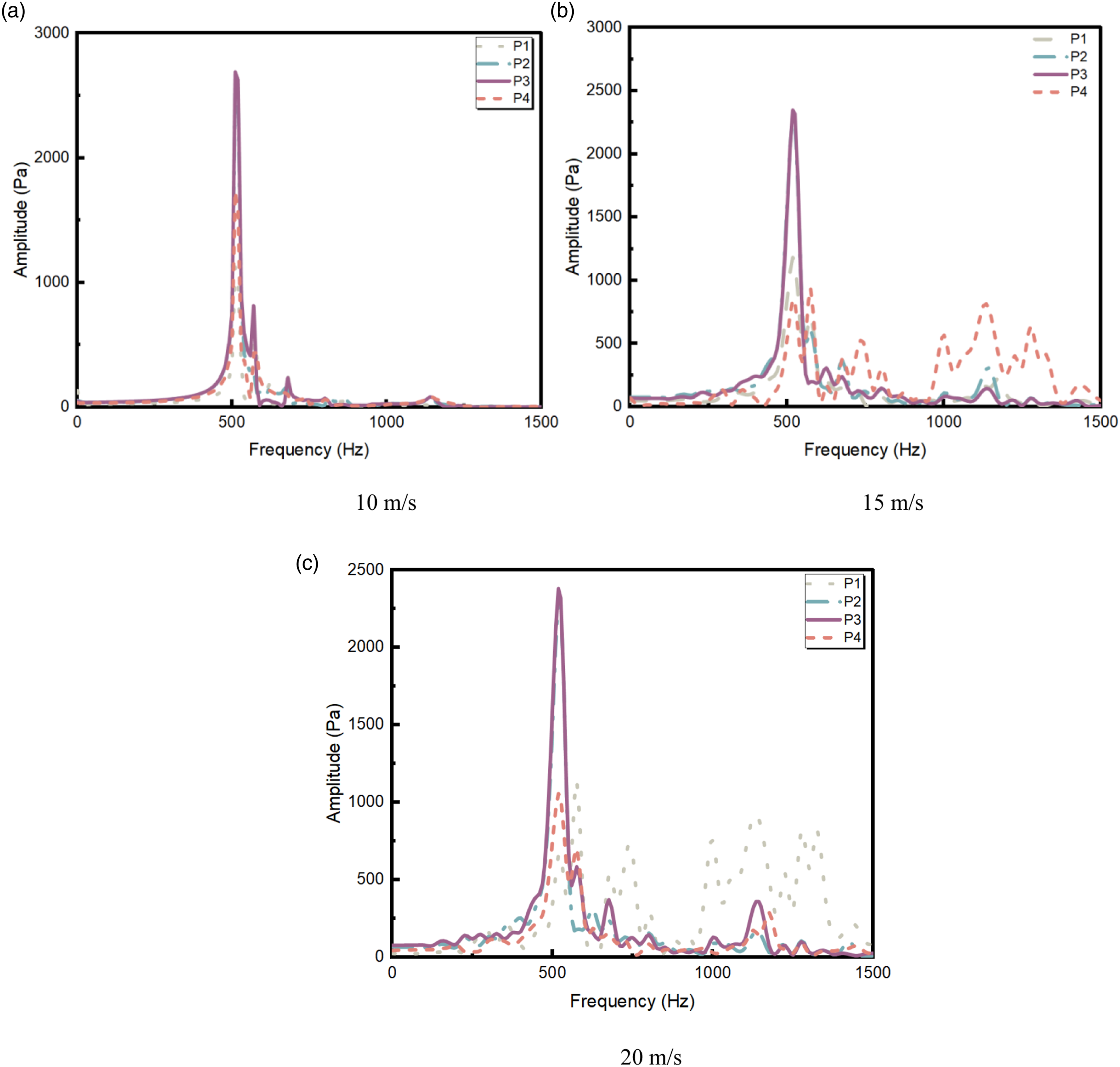

The dissipation effect of acoustic waves at P2 and P3 as time increases was analyzed from a time–frequency perspective, as shown in Figure 15. For point P2, the energy proportion of the fundamental wave increases substantially with rising flow velocities, and the proportions of the first and second harmonics are larger than other cases when flow velocity equals to 15 m/s, demonstrating the strong non-linear effect of the system at this case, further confirming the correctness of the analysis of Figure 14. Besides, it should be mentioned that the energy of the first harmonic is comparable to the fundamental wave at the beginning of combustion, while there exists an energy transmission from the harmonic to the fundamental wave as time rises. The frequency components at P2 and P3 under various flow rates were analyzed, and the proportion of the first harmonic at two points gradually increases with rising velocities, and it also can be found that the more harmonics were excited at P3 than at other points at a case of U_in = 15 m/s, which attenuated and dissipated quickly during transport to P2.

Figure 15.

Time-frequency analysis at monitoring points P2 and P3: (a) U_in = 10 m/s, at point P2, (b) U_in = 10 m/s, at point P3, (c) U_in = 15 m/s, at point P2, (d) U_in = 15 m/s, at point P3, (e) U_in = 20 m/s, at point P2, (f) Uin = 20 m/s, at point P3.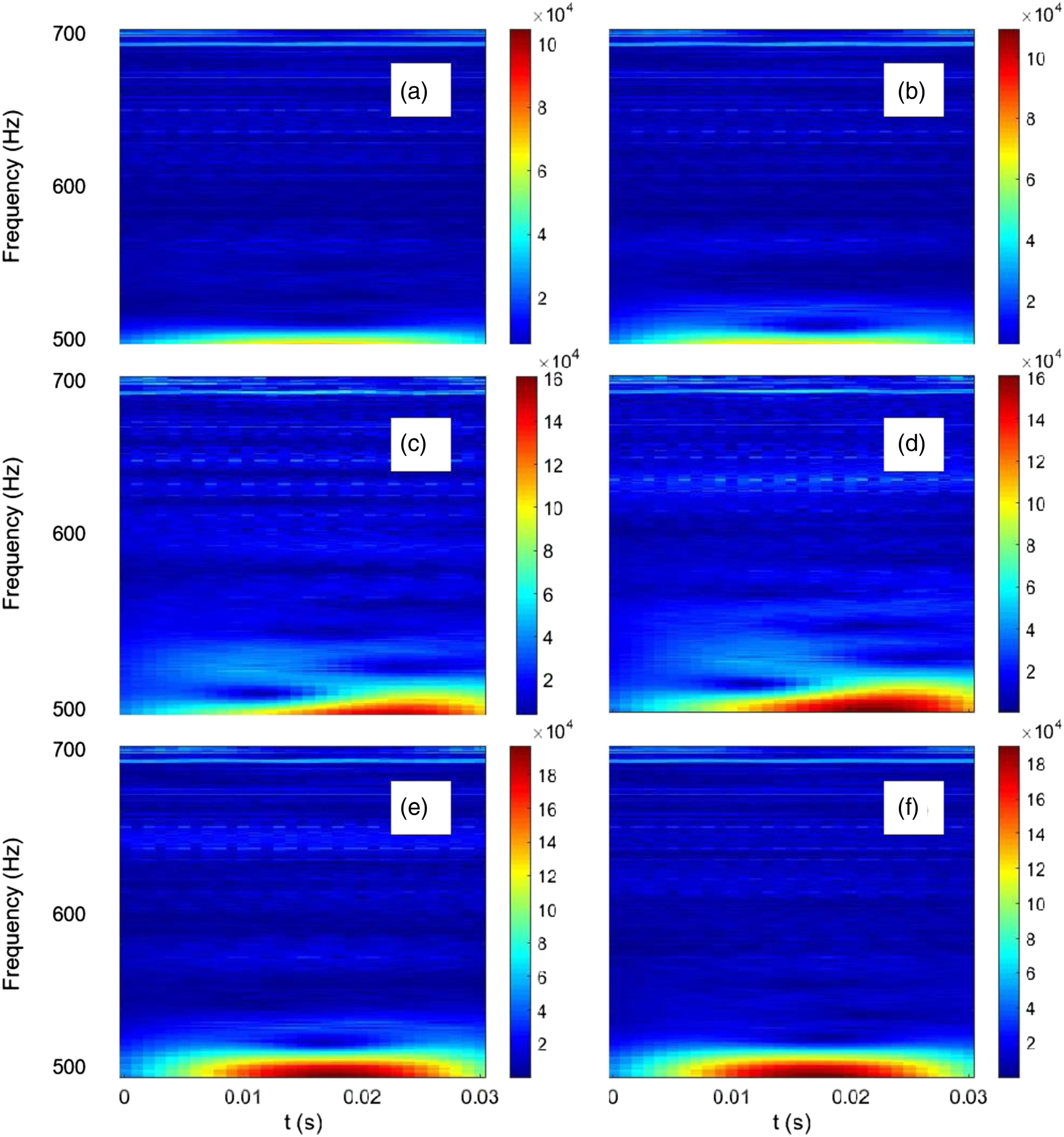

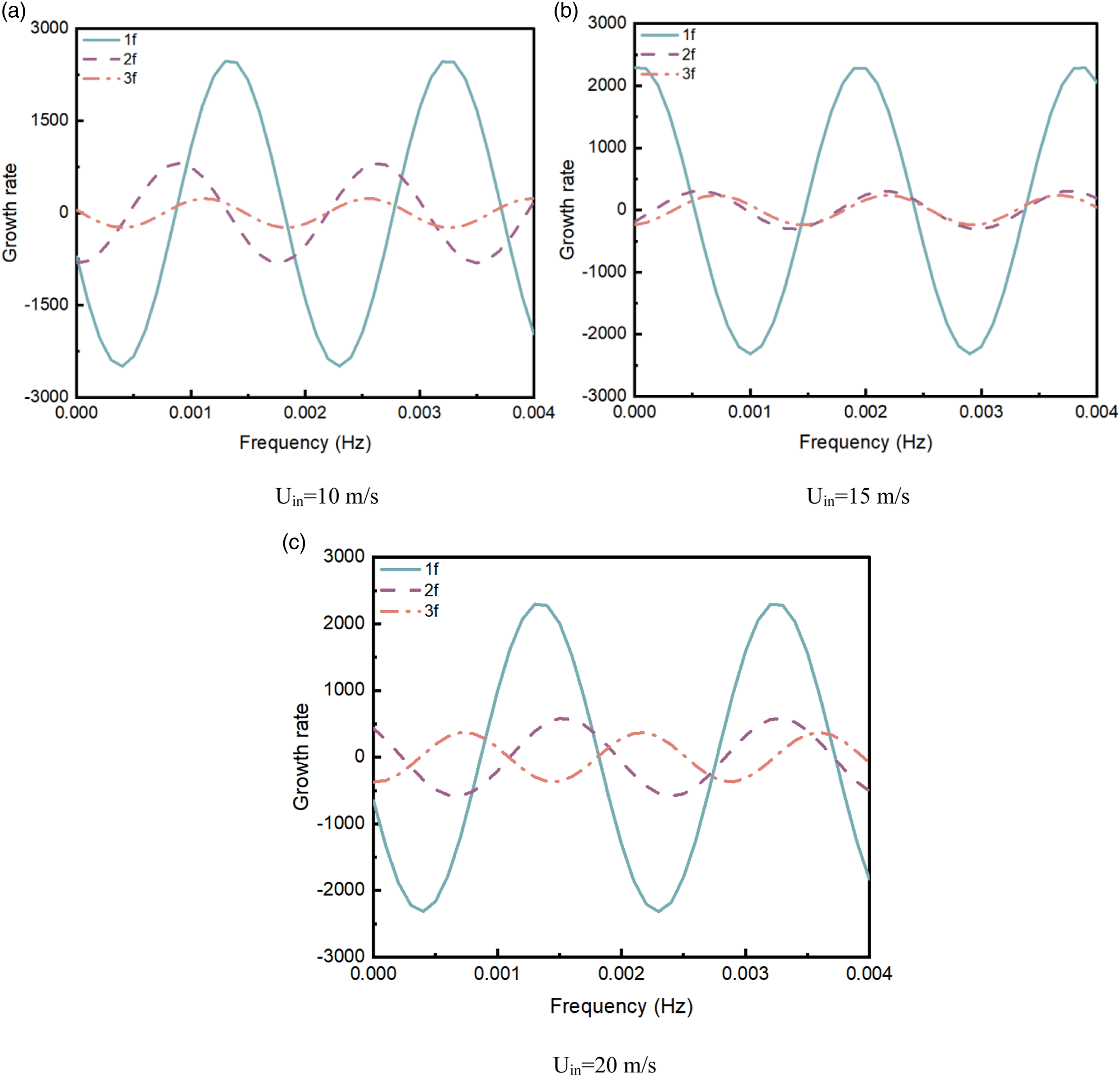
Figure 16 shows the variation of the growth rate of each frequency mode under various inlet velocities. It can be seen that there is a multi-frequency coexistence of complex systems when flow rate equals to 15 m/s, growth or decay rates of high-frequency components occupy a large part of the waves transmitted out of the system, while the frequency components of the transmission under other cases are still dominated by the low-frequency signal of 0–500 Hz. Figure 16(b) and (c) show the growth rates of the frequency components at monitoring points P2 and P3. It can be found that growth rates of various frequencies become larger near 700 Hz with increasing flow velocities, while the variation of growth rate is the smallest at a flow velocity of 15 m/s. It is also worth noting that the corresponding frequency at which the growth rate gets its peak value gradually increases as the transport distance increases, showing that energy of low-frequency gradually transfers to high-frequency during the wave transmission.

Figure 16.

Growth rate of each mode at different inlet flow velocities.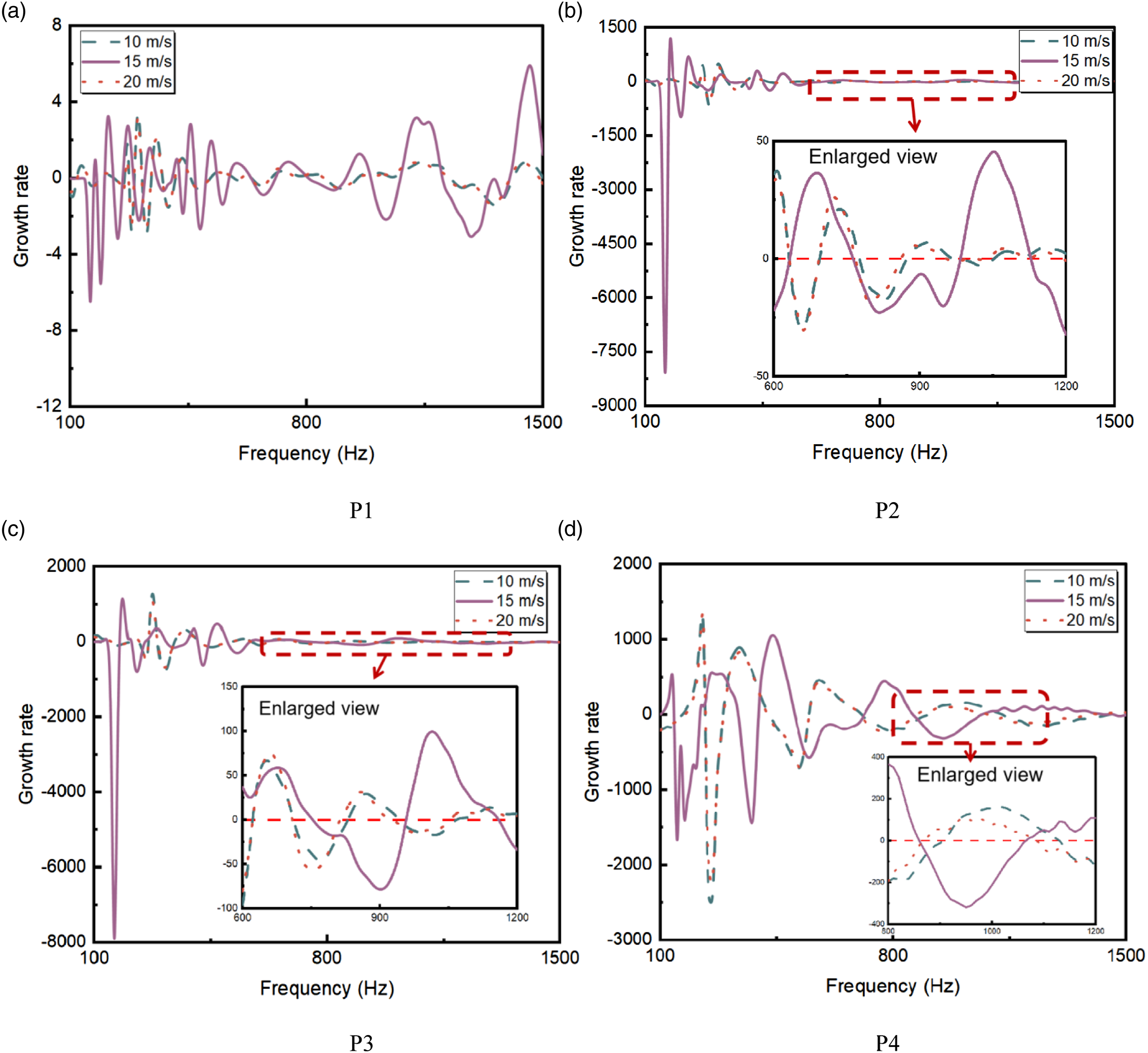

Harmonic analysis and quantitative characterization

The acoustic transmission properties under various methane mass fractions and inlet velocities were investigated from time and frequency perspectives in previous sections. In this section, harmonic analysis was used to deeply analyze the variation law of amplitude and phase of different fundamental modes under different working conditions. Thanks to its high amplitude and complex frequency structures at various cases, the monitoring point P3 becomes the most worthy point for harmonic analysis. Based on the above frequency domain analysis, the first three peak frequencies under various cases at monitoring point P3 were extracted and their fluctuations were plotted, as shown in Figures 17 and 18. Accordingly, in-depth analysis was conducted from the perspectives of amplitude, phase, and model-shape.

Figure 17.

Harmonic analysis at different $w_{CH4}$ .

Figure 18.

Harmonic analysis at different inlet flow velocities.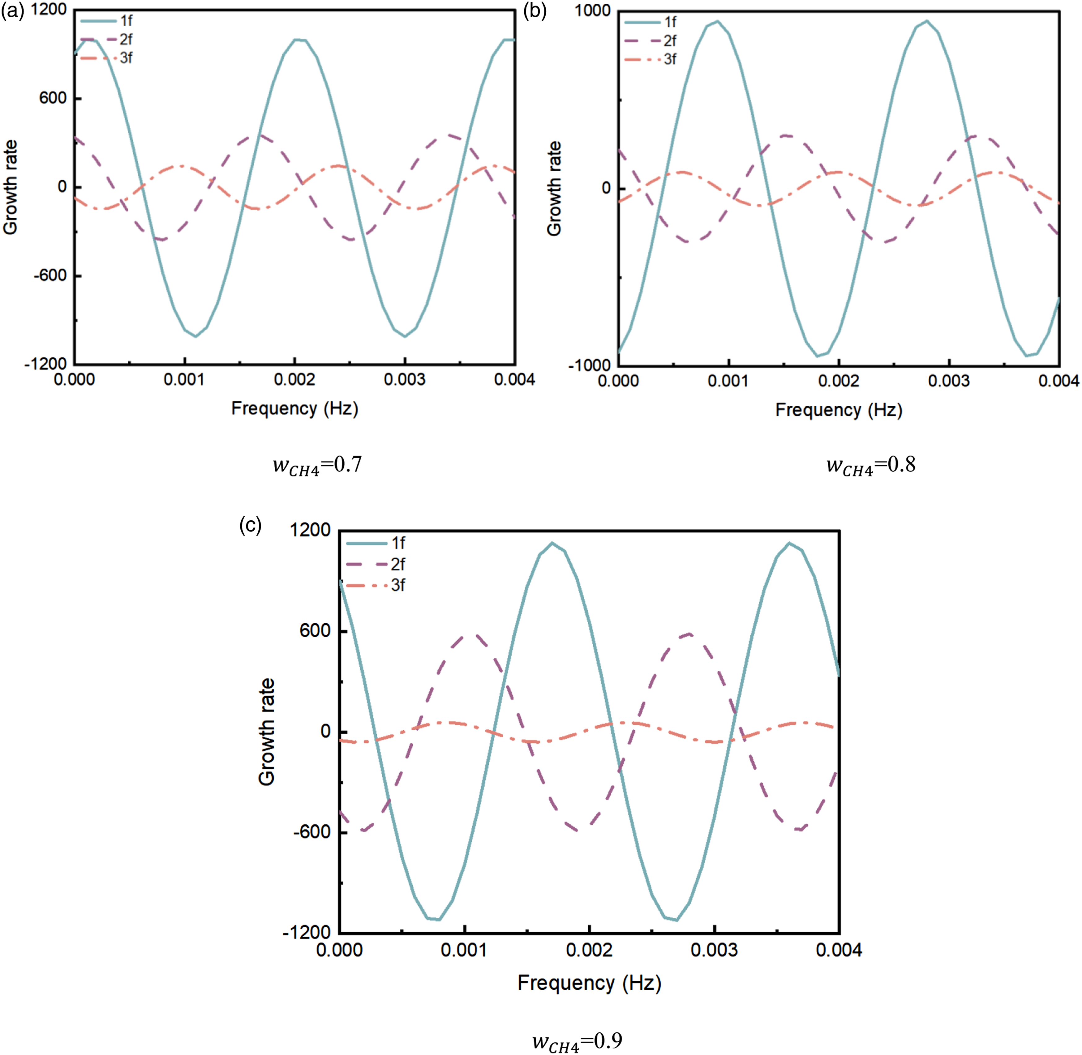

Harmonic analysis

It can be seen from Figure 17 that the amplitude of the harmonics at $w_{CH4}$ = 0.8 greatly decreases compared with other cases. Comparing the amplitude of the harmonics with the fundamental, it can be found that the amplitude of first harmonic is 35.14% of the fundamental at $w_{CH4}$ = 0.7, 52.1% of the fundamental at $w_{CH4}$ = 0.8, and 31.2% of the fundamental at $w_{CH4}$ = 0.9. The fundamental is mainly caused by the compression and expansion of gas in the combustion chamber, and the first and second harmonics are mainly caused by the combustion of gas in the combustion chamber, gas reflow, and gas transportation. That is to say, the larger the proportion of higher harmonics, the greater the impact of the combustion process on the acoustic oscillations. Therefore, it can be concluded from Figure 17 that gas combustion, reflux, and transmission processes have a greatest impact on acoustic oscillation at $w_{CH4}$ = 0.8. Figure 18 illustrates the first three harmonic oscillations when the inlet velocity is 10 m/s, 15 m/s, and 20 m/s. It can be seen that the amplitude of the first and second harmonics at a flow rate of 15 m/s is small compared to the fundamental wave, showing that the expansion and compression of gas at U_in = 15 m/s has a greater impact on the acoustic oscillation.

Phase analysis

From the point of view of phase, it can be seen from Figure 17 that mass fraction of methane has a certain impact on the phase of harmonics; the phase of harmonics increases and the gap between the fundamental and the harmonic becomes larger as mass fraction of methane increases. The possible reason for increasing phase at beginning is that the expansion and compression process of gas is accelerated with an increase of inlet velocity; thus, the initial value of the underlying harmonic becomes larger at the beginning of the cycle, and the curve as a whole is delayed backward. A larger gap between fundamental and harmonics with rising velocities can be accounted for the time required to carry out energy conversion between fundamental and harmonics becomes longer with rising flow rates.

Pressure model-shapes

To shed lights on the acoustic pressure mode-shapes along the central axis, the instantaneous acoustic pressure along the axial directions at different mass fractions and velocities is examined and analyzed. ³⁷ Figure 19 represents the decomposed mode-shapes of the fundamental mode (1f) and the harmonic one (2f). Firstly, the fundamental mode occupies the most important place while the second harmonic is almost non-existent near the inlet of burner. However, when goes to downstream of the burner, it can be clearly observed that the amplitude of the second harmonic dramatically increases then declines, which indicates that there is an energy conversion from low-frequency waves to high-frequency waves in the process of wave transmission. Secondly, it can be viewed from Figure 19(a) that all modes have the lowest amplitude compared with other cases at ${\mathrm{w}}_{\mathrm{C}\mathrm{H}4}$ = 0.8. Besides, it also should be mentioned that a methane mass fraction of 0.8 owns the largest amplitude of the second harmonic at downstream of the burner, emphasizing that the most intense energy conversion among the modes occurs in this case. Model-shapes of two harmonic waves at various velocities can be observed from Figure 19(b). Similar to the previous analysis, the amplitude of the fundamental model is larger than the second harmonic at upstream of the burner, while the second harmonic becomes more important at downstream. Further analysis shows that the amplitude of two models with a velocity of 15 m/s is smaller than others at beginning of the burner. Nevertheless, at the end of the burner, the amplitude of the harmonics rapidly increases at U_in = 15 m/s, indicating that there occurs an energy transformation from low-frequency waves to high-frequency ones during the transmission of sound waves.

Figure 19.

Pressure model-shapes at different conditions.

Conclusions

Based on a model coupling RANS and LNSEs, port analysis, time and frequency domain analysis, wavelet analysis, and harmonic analysis were used to investigate forward propagation, reflection, transmission, and attenuation characteristics of acoustic waves under various inlet velocities and fuel mass fractions. Meanwhile, acoustic waves under various cases were decoupled into individual harmonics for in-depth analysis. The main conclusions of this paper are as follows:

1. The energy distribution of acoustic modes under high-frequency acoustic excitation is more uniform. Acoustic oscillations caused by multiple physical fields are more dramatic than that caused by simple flow field, and the amplitude of the former is 10,000 times higher than that of the latter.

2. The case when $w_{CH4}$ owns the largest percentage of energy conversion from fundamental to high-frequency signals and the largest percentage of transmitted waves from combustion chamber system to outside and the strongest non-linear effect. The amplitude of oscillations at points and the attenuation effect of high-frequency signals along the axial are enhanced with rising $w_{CH4}$ .

3. Compared with other cases, at the case of U_in = 15 m/s, the amplitude of harmonics is reduced by 18%, yet the proportion of the high-frequency harmonic increases, proving the non-linearity cannot be neglected in this case. The energy conversion from fundamental to high-frequency signals enhances with rising velocities. As the flow rate increases closer to the outlet position, the more complex the oscillation signal is.

4. Model-shapes analysis show that the case of $w_{CH4}$ = 0.8 owns the largest amplitude of the second harmonic at downstream of the burner, while the amplitude of the harmonics rapidly increases at U_in = 15 m/s at the end of the burner, which further indicates that the energy conversion of low-frequency signals to high-frequency signals occurs mainly in the middle and downstream regions.