Sage Journals: Discover world-class research

Abstract

Accurate prediction of thermoacoustic instability is a prerequisite for thermoacoustic control to avoid the damage of combustion chamber, however, this problem has not been completely solved yet. This paper proposes a data-driven method based on the Elman neural network (ENN) to predict the value of acoustic pressure of combustion instability. As a comparison, a model based on support vector machine (SVM) was built. It is proved that ENN has better prediction performance with a certain predicted time horizon compared to the SVM method. What is more, the prediction model based on ENN can adapt to time-varying characteristics of the transition scenario which is characterized by amplitude modulation, multiple frequencies, and irregular bursts. ENN model still maintains enough prediction accuracy for various input training sets, indicating that ENN can fully mine the features of data and has a strong feature extraction ability in combustion oscillation prediction. Hence, it is demonstrated that ENN is a promising prediction tool for thermoacoustic instability under various combustion conditions. These findings are of great significance for the accurate prediction and control of thermoacoustic instability.

Keywords

thermoacoustic instability prediction acoustic pressure Elman neural network

Introduction

In the early stage, diffusion combustion was used in the combustion chamber, which has good flame stability.¹ With the increase of gas turbine power, the temperature of the diffusion combustion chamber is getting higher, resulting in the excessive emission of NO_x. To meet more and more stringent emission standards, lean premixed combustion is widely used in modern gas turbines.^2,3 However, a lean premixed combustion chamber is more prone to thermoacoustic oscillations caused by the coupling of combustion heat release rate fluctuation and pressure fluctuation.^4-6 Thermoacoustic oscillations have been frequently encountered in the propulsion systems such as ramjet engines, rocket motors, aero-engine, and land-based gas turbines. There are many kinds of thermoacoustic oscillations. For many operating conditions, a limit cycle oscillation is reached at an essentially fixed oscillation frequency and constant amplitude. In addition to the limit cycle oscillation, there are some other types of combustion oscillations that may occur in certain circumstances. These states, which are defined as amplitude modulation limit cycle here, are characterized by amplitude modulation, multiple frequencies, and irregular bursts.⁷ Kabiraj⁸ has studied the limit cycles and the amplitude modulation limit cycle which include period doubled, quasiperiodic, frequency-locking, and chaotic thermoacoustic instability. Thermoacoustic instability deteriorates the performance and the life of the combustion chamber. Many passive and active methods have been proposed to control thermoacoustic oscillations.^1,9-13 However, the evolution of thermoacoustic oscillation is difficult to track, due to the complex nonlinear characteristics of thermoacoustic oscillation. The real time monitoring of these oscillations remains a serious challenge.

At present, most combustion monitoring systems are designed based on the frequency-domain treatment of a signal.^14,15 And the amplitude of the dominant mode of the acoustic pressure from the Fourier transform spectrum is generally adopted for precursors of combustion instability. However, due to the inherent low-frequency spectral resolution defect of short-time data, the frequency domain transformation of transient signals (such as the dynamic pressure signal at the beginning of combustion oscillation) usually loses the time details of the signal.¹⁶ Therefore, the spectrum analysis of dynamic pressure signals is generally insufficient to identify the transition scenario from a stable state to oscillation. At the same time, a time-domain analysis was proposed. As thermoacoustic instability approaches, roots mean squares and variances of the acoustic pressure increase gradually.^17-19 Song¹⁶ proposed that a combustion process can be quantified using the kurtosis of dynamic pressure signals. However, due to the existence of intermittent oscillation, beat vibration, and other oscillation forms, these measured values do not change monotonically.¹⁸ Therefore, this method is prone to misjudgment and cannot distinguish various oscillation modes. In addition, real-time monitoring is not guaranteed because it takes time to collect and process data. To reserve adequate time for any meaningful control action,²⁰ a combustion oscillation model is established to predict whether thermoacoustic oscillation will occur in the next few seconds. However, the existing theoretical models are not accurate enough because of the complex nonlinearity of thermoacoustic instability.

Data-driven methods based on machine learning tools have drawn the attention of people recently due to their strong learning ability and nonlinear fitting ability. In reference,²¹ a neural ordinary differential equation (neural ODE) is used to model the whole thermoacoustic system. Zhu²² proposed the stacked long short-term memory network (S-LSTM) to predict the amplitude of acoustic pressure signal in the future, and compared with the support vector machine (SVM), S-LSTM achieved good prediction performance. Ruiz²³ performed nonlinear analysis on the sound pressure signal to obtain the thresholdless recurrence plot and then trained the convolutional neural network to predict the beginning of combustion instability. Elman neural network (ENN) is a typical dynamic recurrent neural network and it shows good performance in nonlinear time series prediction. However, to the best of our knowledge, ENN has not been paid attention to in the field of thermoacoustic instability.

In this paper, we first analyzed the complex and changeable modes of thermoacoustic instability based on the experimental data, and then selected the data of the typical operating point as the training and verification data set of the model based on ENN. ENN was used to establish the data-driven model of the thermoacoustic system, which was applied to predict the value of acoustic pressure. Furthermore, a model is constructed by the support vector machine (SVM). The prediction performance of ENN was compared with that of SVM, and the choice of training parameters of ENN was discussed.

Methods

Experimental setup

The experimental device used in this experiment is shown in Figure 1. The acoustic pressure data used in the study were obtained from the Rijke tube. The setup consists mainly of three parts: a flame burner, a borosilicate glass duct, and the measurement system. The burner tube, where fuel (methane) and air are mixed, is made of stainless steel, and 500 mm in length with an inner diameter of 22.5 mm. The length of the glass duct is 750 mm, and the inner diameter is 50 mm. The distance between the flame position and the bottom of the glass tube is 60 mm. There are two holes on the glass tube to measure the pressure signal of the combustion system. To make the sensors work in the appropriate temperature, a semi-infinite pressure tube was adopted in Figure 1. Acoustic pressure data were acquired using two microphones (CRYSOUND type 547). A signal conditioner (PCB 482C16) was employed to amplify the tiny voltage signal, which will increase the accuracy of signal acquisition. And a 16-bit analog-to-digital conversion card (NI 6212) was used to acquire data at a sampling rate of 10 kHz. The oscillation frequency of the combustion system is within 1 kHz, so the digital signal after sampling completely retains the information in the original signal.

Figure 1.

Schematic of the experimental setup.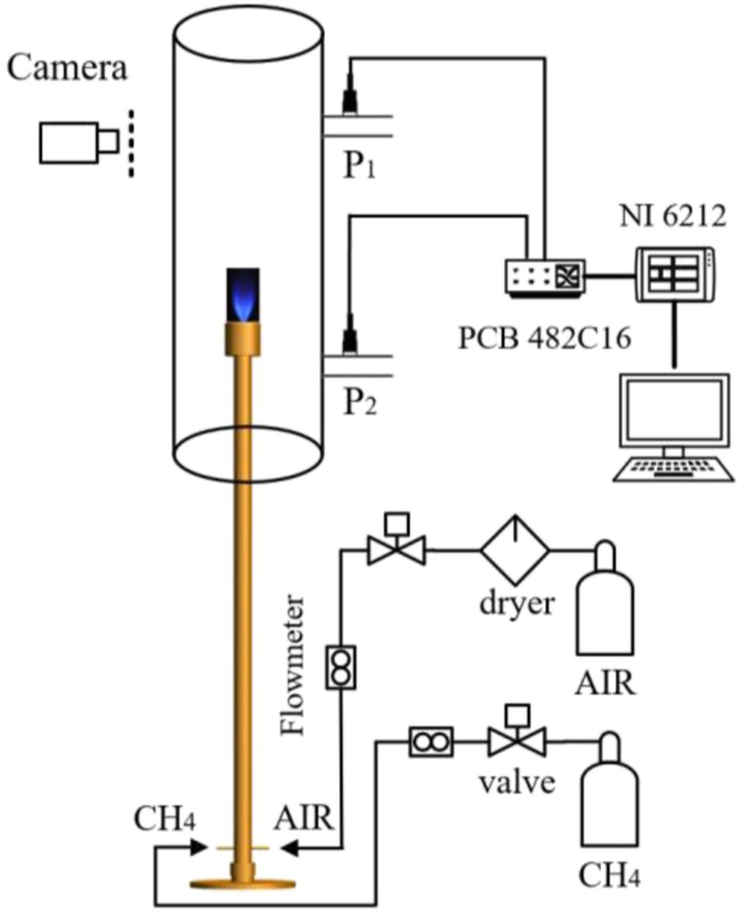

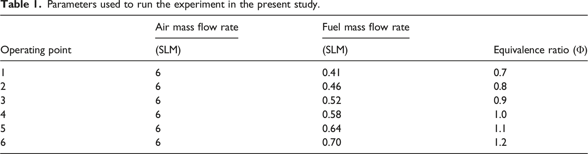
The experimental conditions of this paper are shown in Table 1. The experimental data of six working conditions are collected in this paper. During the experiment, keep the airflow 6 SLM (standard liter per minute) and increase progressively the equivalence ratio by 0.1. The acoustic pressure data of every working condition is recorded. The equivalence ratio range is 0.7–1.2. In our previous experiments, it was proved that thermoacoustic oscillation hardly occurs under other equivalent ratio conditions.

Table 1.

Parameters used to run the experiment in the present study.

Operating point	Air mass flow rate	Fuel mass flow rate	Equivalence ratio (Φ)
Operating point	(SLM)	(SLM)	Equivalence ratio (Φ)
1	6	0.41	0.7
2	6	0.46	0.8
3	6	0.52	0.9
4	6	0.58	1.0
5	6	0.64	1.1
6	6	0.70	1.2

Nonlinear analysis methods

Combustion thermoacoustic instability is an inherent nonlinear characteristic. Therefore, if we want to fully understand this process, we must determine the intermediate dynamic states of the system, such as periodic limit cycle oscillation, quasi-periodic oscillation, and chaotic oscillation.²⁴ This study mainly uses phase space reconstruction and Poincare section to analyze the dynamic characteristics of combustion instability under different equivalence ratios.

According to Takens delay embedding theorem,²⁵ if we get an observable time series $[x_{1}, x_{2}, x_{3}, . . ., x_{N}]$ measured at a system, we can construct a new vector $[x (i), x (i + τ), x (i + 2 τ), . . ., x (i + (d - 1) τ)]$ ; where, $τ$ is time delay, $d$ is embedding dimension, and $i = 1,2,3, \dots, N - (d - 1) τ$ . In this way, we embed the time series into a d-dimensional phase space. The evolution of this time series trajectory is usually represented by a phase diagram. In addition, we need to choose the optimum delay time ( $τ$ ) and embedding dimension ( $d$ ). There are two frequently used methods for the optimal time delay required to reconstruct the phase space: the autocorrelation function (ACF) method²⁶ and the average mutual information (AMI) method.²⁷ AMI is used to evaluate the correlation between $x (i)$ and $x (i + τ)$ at a given $τ$ . It is a version of the autocorrelation function in a broad sense. The first local minimum of AMI is chosen as the optimum $τ$ in the paper. As for the optimum embedding dimension used for the reconstructed phase space, the common methods are false nearest neighbors (FNN)²⁸ and Cao’s method.²⁹ FNN method must depend on the choice of threshold. It gets different embedding dimensions when different thresholds are used. To overcome this issue, Cao’s method has been chosen in the following data analysis. Based on the above methods, the optimum delay time ( $τ = 0.5 m s$ ) and embedding dimension ( $d = 10$ ) shown in Figure 2 were selected to embed the pressure time series into a higher-dimensional phase space. The Poincare section^{30, 31} is a new phase diagram visualization method, which further reduces the dimension of the system and extracts more concise information. It is used to reveal various forms of motion of the dynamic system such as period doubled, quasiperiodic, frequency-locking, and chaotic thermoacoustic instability in this paper.

Figure 2.

Calculation of AMI method (a) and Cao’s method (b) for phase space reconstruction of pressure time series.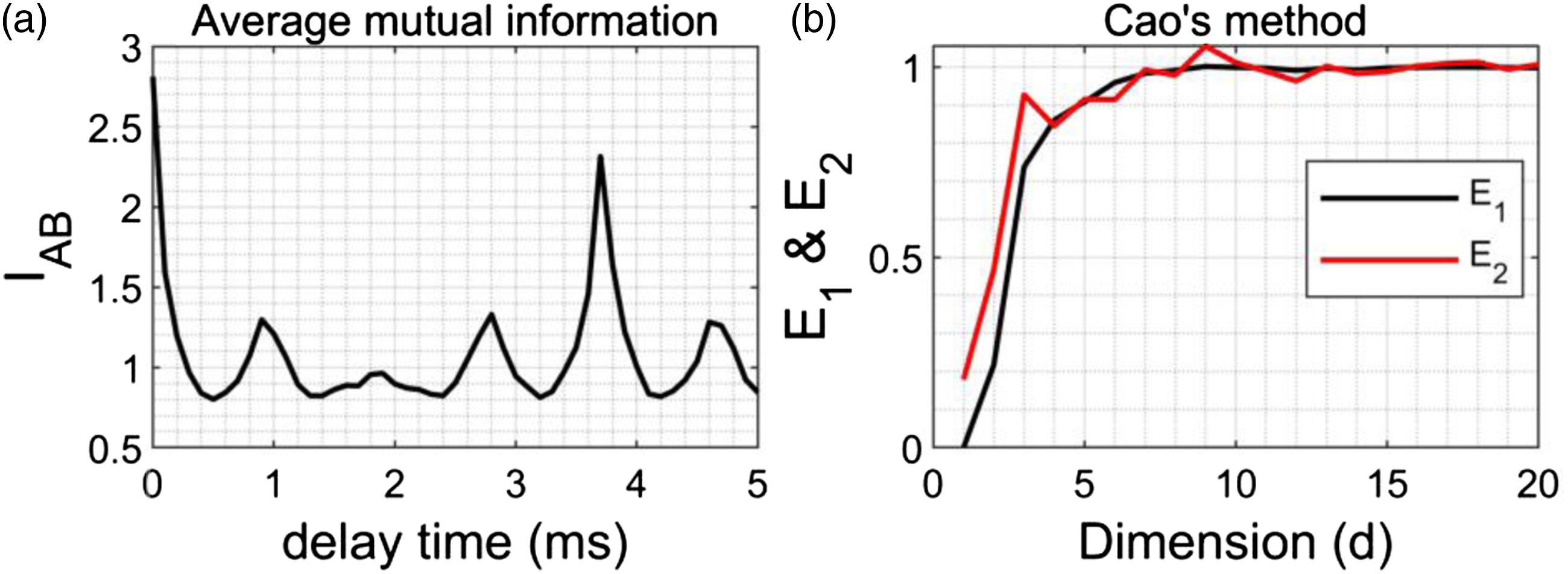

Description of the Elman neural network framework

Elman neural network (ENN) was proposed for speech processing in 1990.³² The structure of ENN is shown in Figure 3. The basic ENN is composed of an input layer, hidden layer, context layer, and output layer. Compared with the BP network, there is an additional context layer in the structure, which is used to form local feedback. The transfer function of the context layer is a linear function, and there is a delay unit, so the connection layer can remember the past state and it was used as the input of the hidden layer together with the input of the network. Therefore, the network has the function of dynamic memory, which is very suitable for time series prediction.

Figure 3.

Schematic of the Elman neural network structure.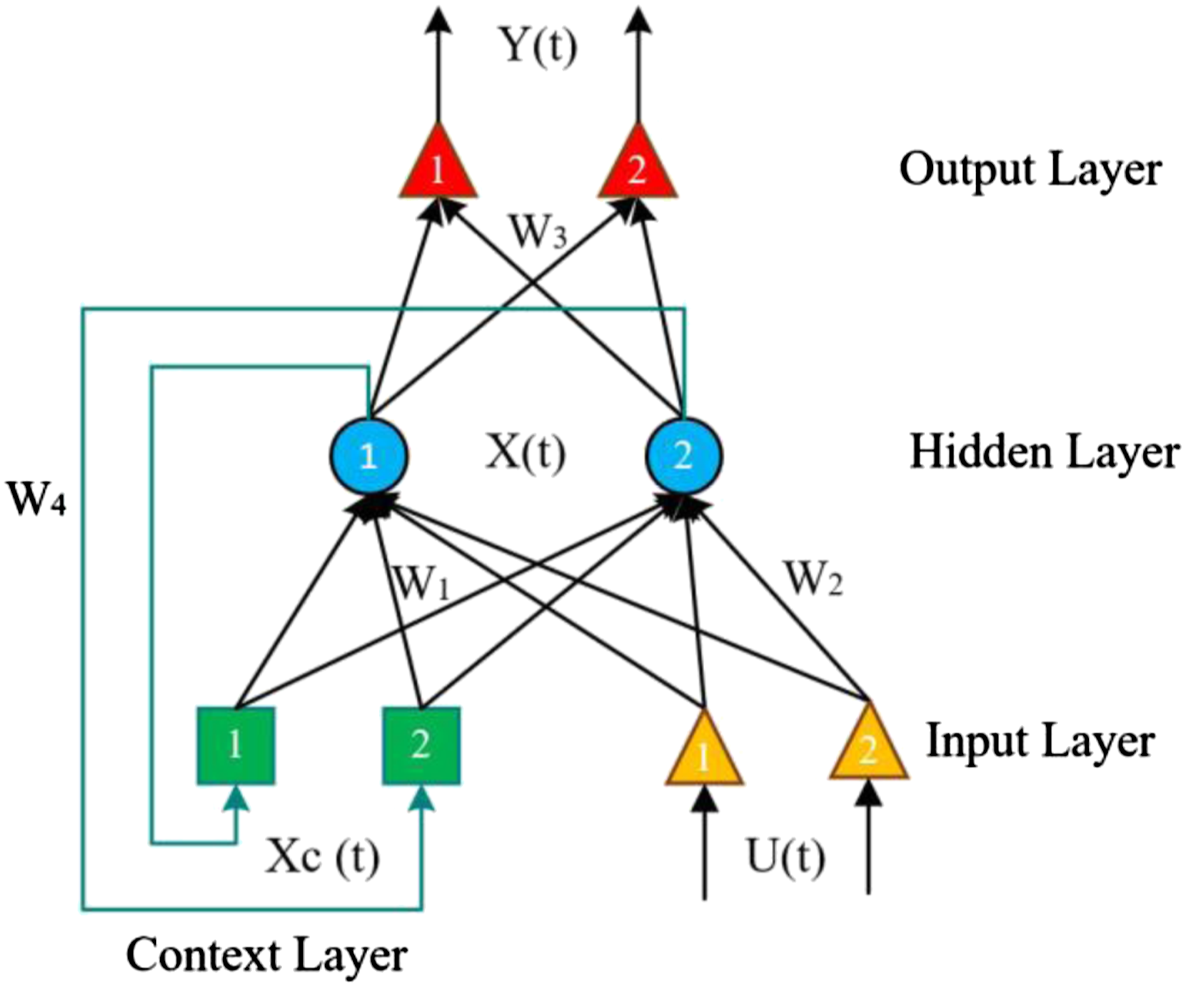

ENN can be described by the following formula (2.1)–(2.3)

X (t) = f (W_{1} X_{c} (t) + W_{2} U (t))

(2.1)

X_{c} (t) = W_{4} X (t - 1)

(2.2)

Y (t) = g (W_{3} X (t))

(2.3)

where the input and output data of the data sets are expressed as

U (t)

and

Y (t)

; the output of the hidden layer and the input of the context layer are

X (t)

and

X_{c} (t)

; the weights between different layers are

W_{1}

W_{2}

W_{3}

, and

W_{4}

, respectively;

f (*)

and

g (*)

stands for the activation function of the ENN in the hidden layer and the output layer.

In this paper, the acoustic pressure time series measured through the microphone is the training data and test data of ENN. In section, the training set is the acoustic pressure data when Φ = 0.9, a limit cycle oscillation case. The experimentally measured data in different cases (Φ = 0.8, Φ = 1.0, Φ = 1.2) is the training and verification data set. In section, the training set is the acoustic pressure data when Φ = 1.1, the amplitude modulation limit cycle oscillation case. The experimentally measured data in different cases (Φ = 0.8, Φ = 1.0, Φ = 1.2) is the training and verification data set. The previous $L$ discrete data were used to predict the next data value. The mapping relationship can be expressed as $x (n) = h (x (n - 1), x (n - 2), x (n - 3), . . ., x (n - L))$ . The number of input layer neurons is equal to that of input variables. The number of output layer neurons is equal to that of output variables and the transfer functions of the output layer and hidden layer are linear functions. The number of context layer neurons is equal to that of hidden variables. The number of hidden layer neurons in the ENN is 25, and the activation function is sigmoid. The maximum number of iterations for the training network is 3000. The permissible error of training termination is 0.0001. The root-mean-squared error (RMSE), which is defined in equation (1), is employed to assess the performance between experimental and predicted pressure time series. The smaller the $E_{R M S}$ is, the more accurate the prediction model is

E_{R M S} = \sqrt{\frac{1}{n} \sum_{i = 1}^{n} {(x_{i} - {\hat{x}}_{i})}^{2}}

(1)

Results and Discussion

Analysis of the experimental dataset

With the increase of equivalence ratio shown in Table 1, the combustion system transits from the stable state to the thermoacoustic oscillation state. The corresponding relationship between the combustion state and working condition is: The combustion system is stable when Φ = 0.7, Φ = 0.8; The combustion system is the limit cycle oscillations when Φ = 0.9, Φ = 1.0; The combustion system is the amplitude modulation limit cycle when Φ = 1.1, Φ = 1.2.

As shown in Figure 4, the acoustic pressure of the stable state is less than 5 Pa, and there is no obvious dominating frequency. The signal collected at this time is the system noise. The thermoacoustic oscillation includes two forms of oscillation in this experiment: Figure 4(b) limit cycle oscillations and Figure 4(c) amplitude modulation limit cycle. The limit cycle oscillations have a basically constant oscillation amplitude of 75 Pa, and the frequency spectrum shows a single dominating frequency of 530.5 Hz. The short-time Fourier transform demonstrates that the dominating frequency of 530.5 Hz isn’t time-variant at this equivalence ratio. As for the amplitude modulation limit cycle, the amplitude of acoustic pressure changes with time, and the frequency of amplitude change is 5 Hz. The frequency spectrum shows the major peak is 270 Hz along with its higher harmonics 540 Hz and 810 Hz, which is different from 530.5 Hz of the limit cycle state. There are two peaks 265 Hz and 275 Hz near 270 Hz. The difference between the three peaks is 5 Hz, which is equal to the frequency of amplitude change. The same phenomenon occurs at 540 Hz. The previous research³³ revealed that there will be several peaks near the main frequency of the beating oscillations, and the frequency interval between adjacent peaks is equal, which is equal to the frequency of amplitude change. These characteristics are the same as those observed in our experiments.

Figure 4.

The diagrams of time domain (a, b, c), short-time Fourier transform (d, e, f) and frequency domain (g, h, i): steady state (a, d, g), limit cycle oscillations (b, e, h) and amplitude modulation limit cycle (c, f, i).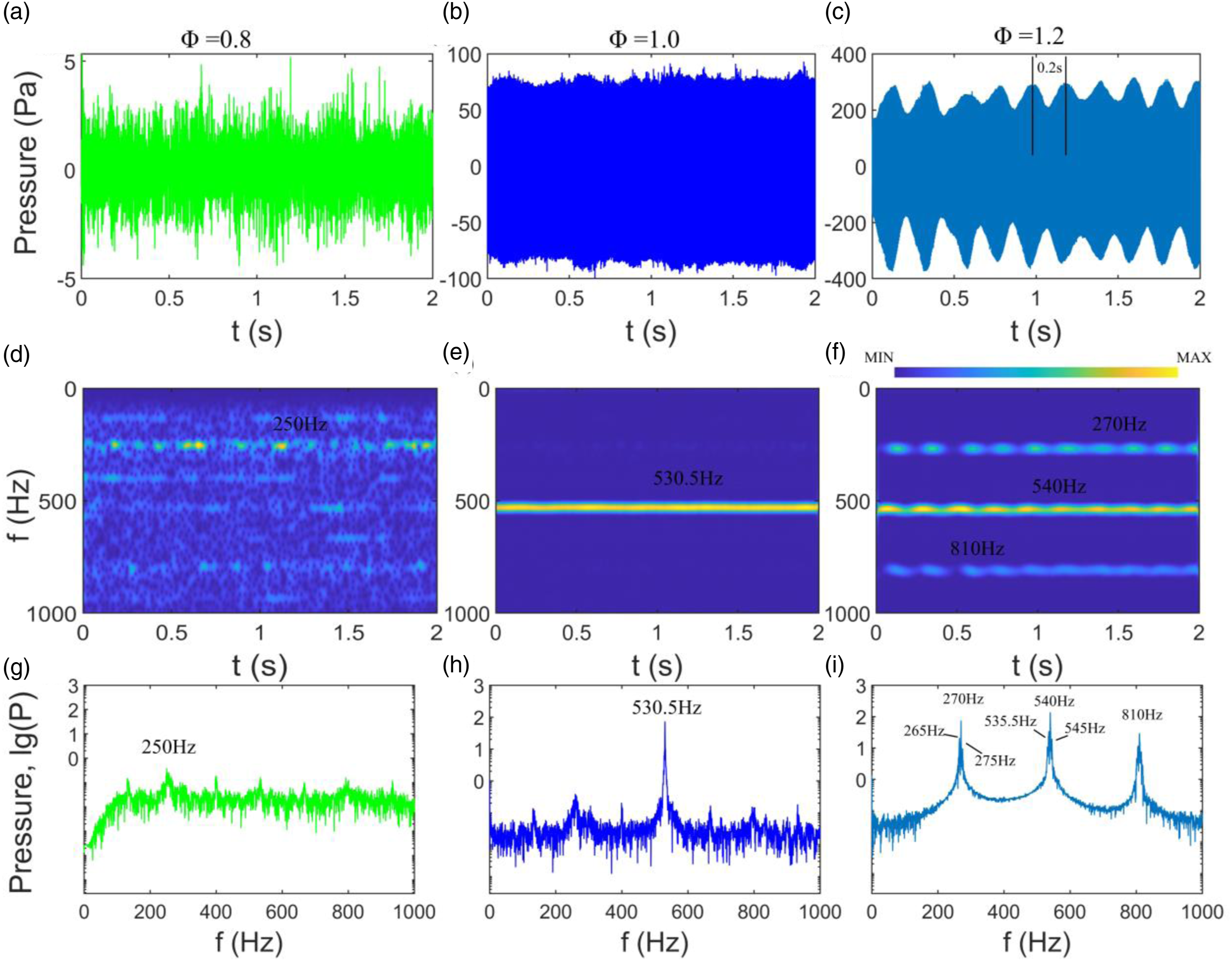

Thermoacoustic systems are complex nonlinear systems. In unstable states, there are different types of oscillations in the system. Time series data, phase plots, and Poincare sections are carefully examined to identify the various attractors in Figure 5. The stable state corresponds to Figure 5(a), (d), and (g), giving the time series of this state, the phase plots, and Poincare sections. The time series of the acoustic pressure are random, which can be considered as system noises. The 3D phase plot of the stable state is a noisy cluttered attractor that does not have any definite geometric structure. As can be seen from the Poincare sections in the Figure 5(g), the distribution of points appears random without any regular pattern. As for limit cycle oscillation which corresponds to Figure 5(b), (e), and (h), the amplitude of the acoustic pressure is basically a constant and the phase portrait of the limit cycle state appears to be an ellipse. If the value of the time delay changed, the phase portrait would look like a circle. As a result of noise in the system, small fluctuations can be seen in the closed-loop trajectory of the limit cycle attractor. The Poincare section shows a single point which is a characteristic of the limit cycle state. The amplitude modulation limit cycle which corresponds to Figure 5(c), (f), and (i), the time series of the acoustic pressure has two amplitudes and change with time. An orbit forms two loops on the phase plot and an enclosed dense circle in two dimensions is shown in the Poincare section. After synthesizing the information above, the amplitude modulation limit cycle in this paper is quasiperiodic oscillations.

Figure 5.

Time series (a, b, c), 3D phase plot (d, e, f) and Poincare section (g, h, i) for pressure oscillations: steady state (a, d, g), limit cycle oscillations (b, e, h) and amplitude modulation limit cycle (c, f, i).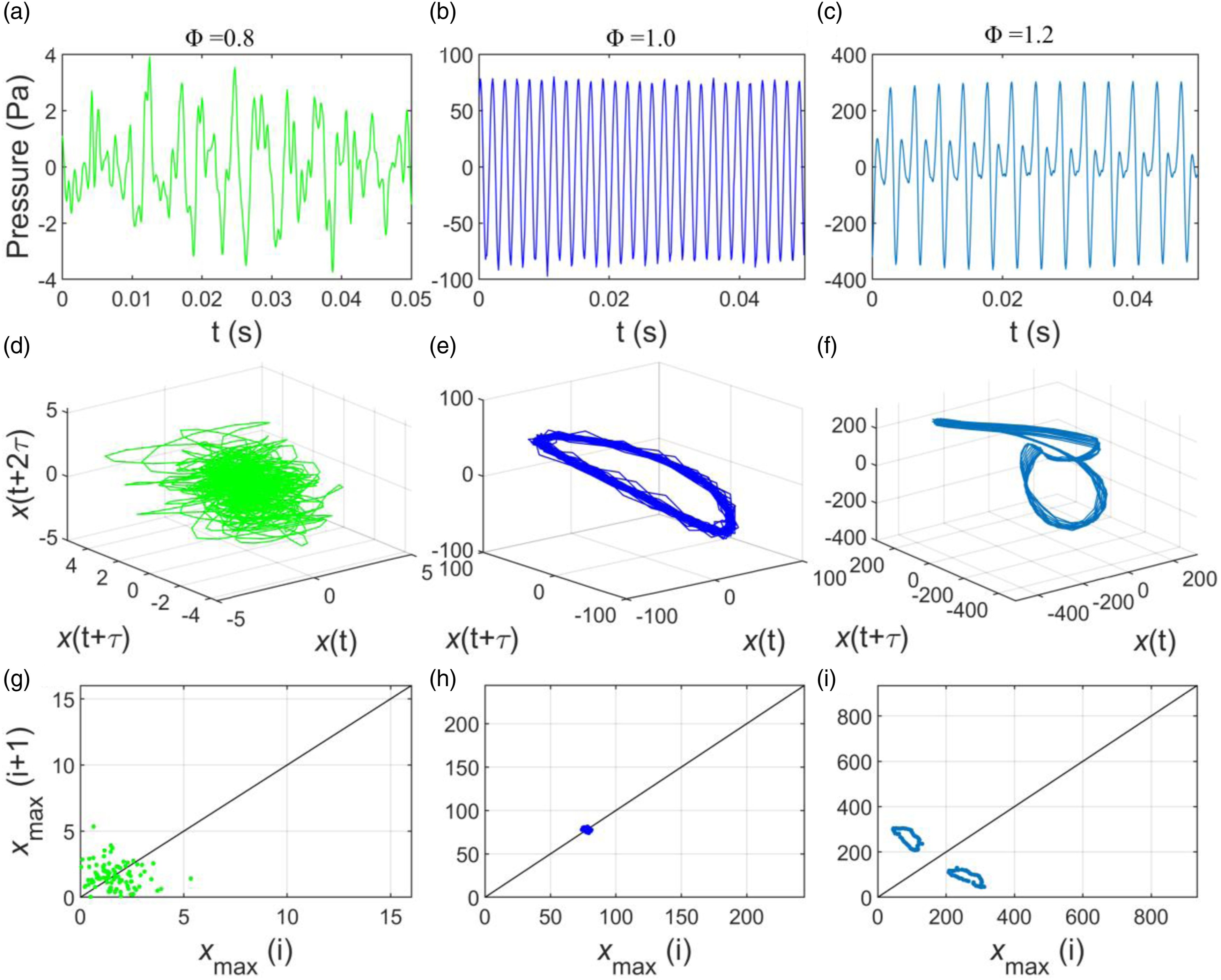

Based on the above analysis, we find that thermoacoustic instability is characterized by amplitude modulation, multiple frequencies, and irregular bursts. When a control parameter was changed, the system displayed periodic, quasiperiodic, or chaotic states. We have encountered great challenges in establishing its mechanism model to predict acoustic pressure because of the complex and variable nonlinearity of thermoacoustic instability. The data-driven methods with strong learning ability and nonlinear fitting ability will be discussed below.

Predicted performance of acoustic pressure

Single-point prediction performance

The single-point prediction means that the previous $L$ discrete data were used to predict the next one data. The mapping relationship can be expressed as $x (n) = h (x (n - 1), x (n - 2), x (n - 3), . . ., x (n - L))$ . Here, $L$ is equal to 50. Figure 6 displays single-point prediction performance in different cases (Φ = 0.8, Φ = 1.0, Φ = 1.2). The experimentally measured data, the data predicted by ENN, and the data predicted by SVM are represented by black, red, and green curves, respectively. As can be seen in Figure 6(a), when Φ = 0.8, the combustion system is stable, so the measured signal is a noise signal that cannot be accurately predicted. As the equivalence ratio increases to Φ = 1.0 shown in Figure 6(b), the limit cycle oscillation occurs. The $E_{R M S}$ of ENN and SVM is $E_{_E N N}$ = 2.6 Pa, $E_{_S V M}$ = 2.8 Pa, respectively, so both ENN and SVM can accurately predict the sound pressure of the limit cycle oscillation. When the equivalence ratio is 1.2, the mode of combustion oscillation is transformed into the amplitude modulation limit cycle. Compared with SVM ( $E_{_S V M}$ = 97.2 Pa), the data predicted by ENN ( $E_{_E N N}$ = 53.1 Pa) is more accurate as shown in Figure 6(c). The training dataset is the sound pressure when Φ = 0.9 that corresponds to the limit cycle oscillation state. So, SVM performs well in predicting limit cycle oscillation modes (Φ = 1.0). However, when the oscillation mode is changed to the amplitude modulation limit cycle oscillation (Φ = 1.2), the prediction result of SVM is completely unreliable. In contrast, ENN has reliable performance in two oscillation modes, indicating that ENN has good generalization ability in combustion oscillation prediction.

Figure 6.

Single-point prediction performance in different cases (Φ = 0.8, Φ = 1.0, Φ = 1.2).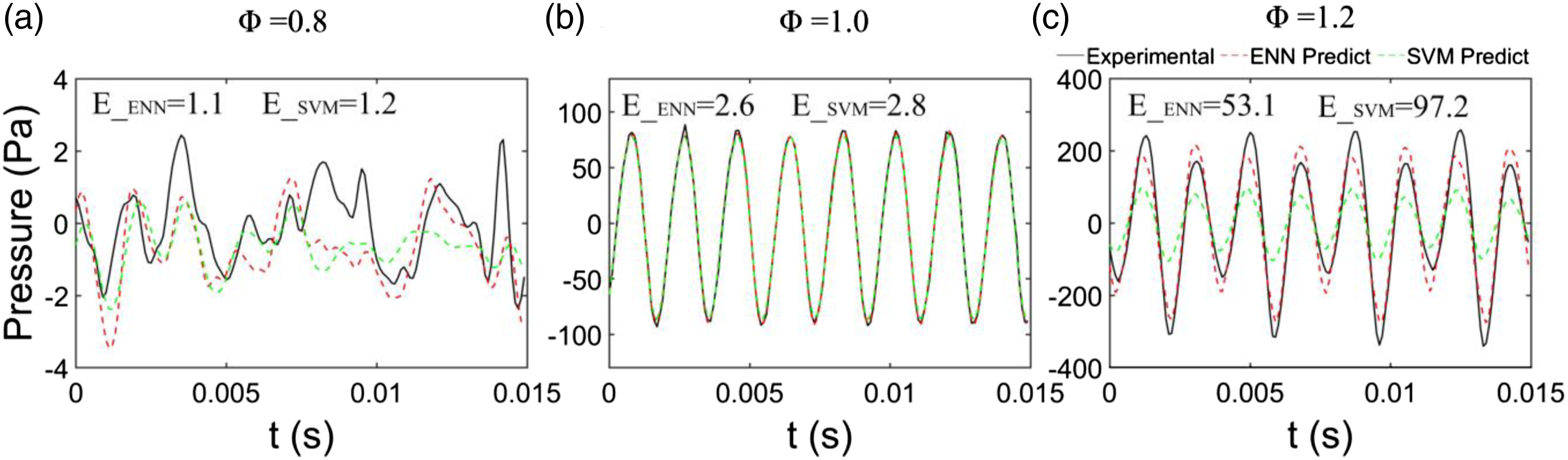

Long-term prediction performance

The long-term prediction means that the previous $L$ discrete data were used to predict the next $R$ future time points. The mapping relationship can be expressed as $x (n), x (n + 1), . . ., x (n + R - 1) = h (x (n - 1), x (n - 2), x (n - 3), . . ., x (n - L))$ . Here, $L$ is equal to 50. Figure 7 displays Long-term prediction performance in different cases (Φ = 0.8, Φ = 1.0, Φ = 1.2) when $R$ is equal to 20. The prediction accuracy of R = 20 is reduced relative to that of R = 1. As for SVM, the $E_{R M S}$ increased from $E_{_S V M}$ = 2.8 Pa (Φ = 1.0), $E_{_S V M}$ = 97.2 Pa (Φ = 1.2) to $E_{_S V M}$ = 35.3 Pa (Φ = 1.0), $E_{_S V M}$ = 101.4 Pa (Φ = 1.2). Meanwhile, the $E_{R M S}$ increased from $E_{_E N N}$ = 2.6 Pa (Φ = 1.0), $E_{_E N N}$ = 53.1 Pa (Φ = 1.2) to $E_{_E N N}$ = 21.5 Pa (Φ = 1.0), $E_{_E N N}$ = 64.4 Pa (Φ = 1.2). When the type of thermoacoustic oscillation is the limit cycle oscillation (Φ = 1.0), the prediction accuracy of SVM is reduced, but still possesses certain engineering application value. The prediction result of SVM is still unreliable in the amplitude modulation limit cycle oscillation mode (Φ = 1.2) as shown in Figure 7. Even though the prediction accuracy of ENN is somewhat reduced, it still performs well in both oscillation modes. ENN shows a powerful ability to extract the characteristic of nonlinearity data. It is demonstrated that ENN still has good generalization ability in the long-term prediction of combustion oscillation.

Figure 7.

Performance of Long-term prediction with a predicted time horizon up to 20 future time points in different cases (Φ = 0.8, Φ = 1.0, Φ = 1.2).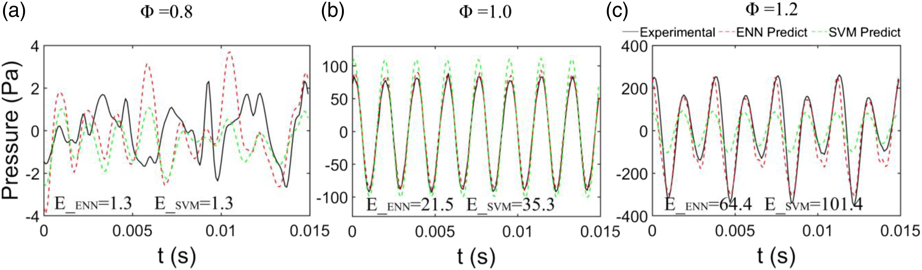

To further test the long-term forecasting ability of the model, we increased the predicted time horizon from 1 point to 100 points. Figure 8 summarizes the $E_{R M S}$ curve, which represents the predictive ability more intuitively. The $E_{R M S}$ of ENN and the $E_{R M S}$ of SVM are represented by red and black curves, respectively. $E_{_E N N}$ is consistently smaller than $E_{_S V M}$ in the three states of the combustion system (Φ = 0.8, Φ = 1.0, Φ = 1.2). It proves that ENN has higher prediction accuracy in a longer predicted time horizon and different combustion states. The combustion system is stable when Φ = 0.8, and the measured signal is a noise signal that cannot be accurately predicted. Therefore, there is no regular relationship between the root mean square and the predicted time horizon. When the limit cycle oscillation occurs, the prediction errors of both ENN and SVM increase with the predicted time horizon. Even though the prediction accuracy of SVM is reduced, the prediction results of both ENN and SVM still possesses certain engineering application value as shown in Figure 7. When the amplitude modulation limit cycle oscillation occurs, the root mean square errors of SVM hardly change with the predicted time horizon and is always large. As for ENN, the prediction errors increase with the predicted time horizon. This shows that ENN can maintain good predictive performance within a certain predicted time horizon in various oscillation modes, to meet the engineering requirements for combustion stability monitoring and control. This may be attributed to the dynamic memory of ENN.

Figure 8.

Statistical 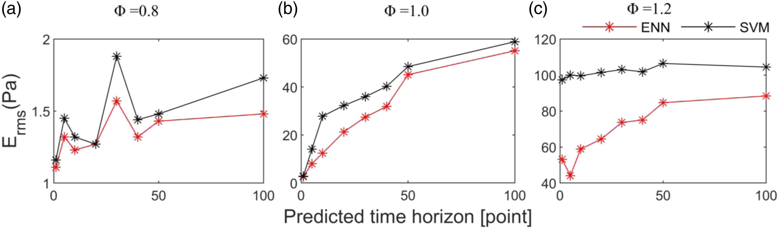$E_{R M S}$ of long-term prediction in different cases (Φ = 0.8, Φ = 1.0, Φ = 1.2).

Prediction of the transition scenario

The actual combustion conditions will change according to the actual needs, and the combustion system may also be affected by various disturbances. Therefore, we need a sound pressure prediction algorithm that can track the changes in the combustion state. The algorithm is expected to not only accurately predict the combustion mode but also accurately predict the transition states which contain the process from stable state to unstable oscillating and transitions between various oscillating states. The following experiments show that ENN can meet these requirements. Figure 9 shows the predicted performance of transition scenarios. The experimentally measured data, the data predicted by ENN, and the data predicted by SVM are represented by blue, red, and green curves, respectively. As shown in Figure 9(a), the amplitude of thermoacoustic oscillation changes with the change of equivalence ratio and external disturbance. The whole data set can be divided into three stages: The first stage, shown in Figure 9(b), is a nonperiodic oscillation and the amplitude is small. The second stage, shown in Figure 9(c), is the transition states. The amplitude of thermoacoustic oscillation increases gradually in this stage. The third stage, shown in Figure 9(d), is the periodic limit cycle oscillation. The amplitude of thermoacoustic oscillation is kept in a large range. The pressure predicted by ENN always changes synchronously with the experimental value and the predicted value is the same as the experimental value. This proves ENN’s perfect predicted performance of transition scenarios. As for SVM, it can accurately predict the amplitude at the beginning of oscillation, but it cannot adapt to the change of combustion state. In some stages, the results predicted by SVM are contrary to the experimental results and it is completely unable to meet the monitoring and control requirements. Thanks to the context layer and local feedback structure of the ENN, ENN has a short-term memory function, so the prediction model is adapted to time-varying characteristics.

Figure 9.

Predicted performance of transition scenarios.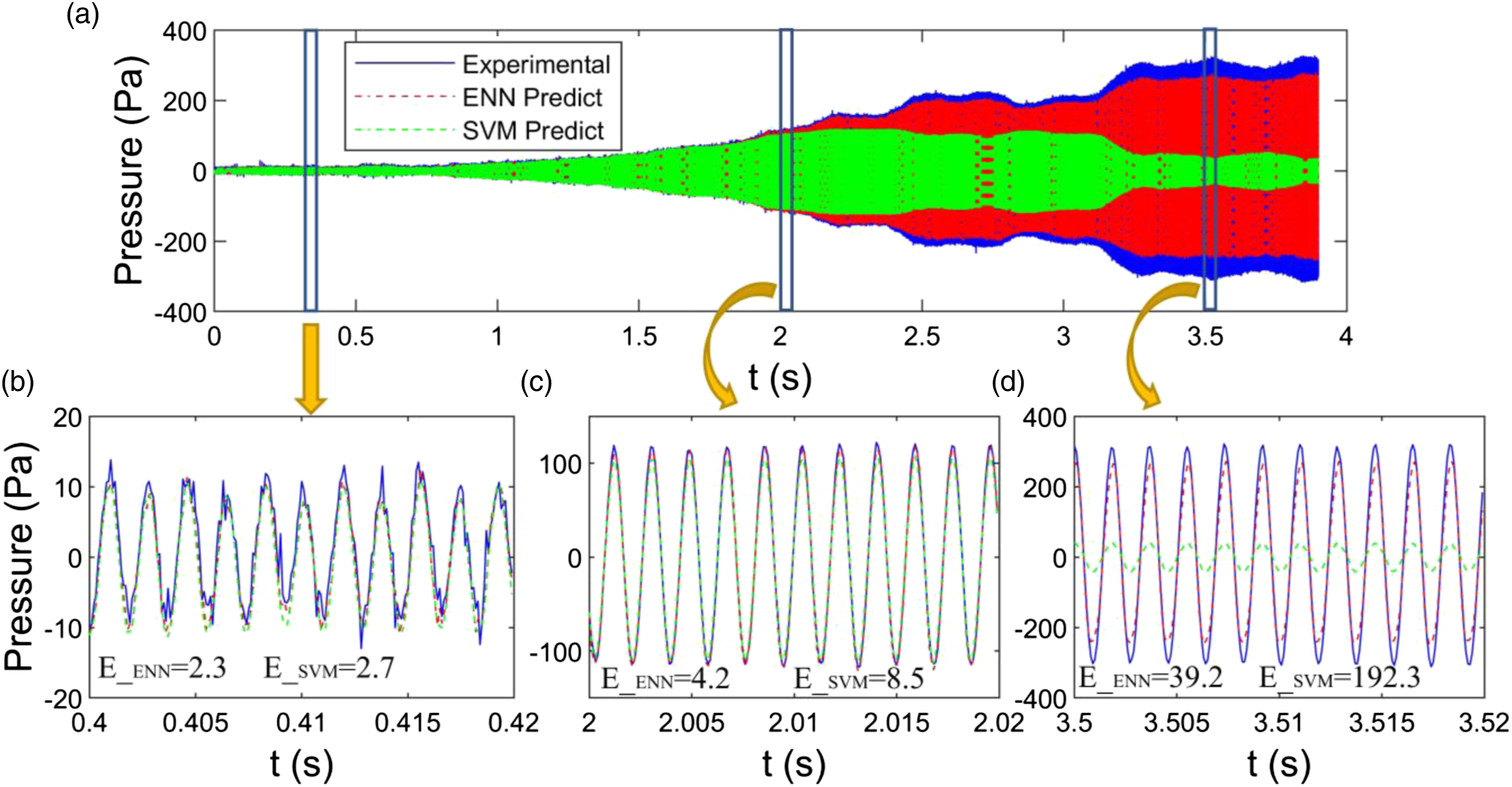

Influence of input choice on the Elman neural network

Choice of the input training set

The input training set has a great influence on the accuracy of neural network model. If the distribution of the data class is unreasonable, it will lead to insufficient training. The training set in Section only contains the sound pressure data when Φ = 0.9, a limit cycle oscillation case. In this section, the sound pressure data of the amplitude modulation limit cycle oscillation (Φ = 1.1) is used to train the neural network model. Other configurations are the same as those in Section. Single-point prediction performance is shown in Figure 10. For SVM, the $E_{R M S}$ increased from $E_{_S V M}$ = 2.8 Pa (Φ = 1.0) to $E_{_S V M}$ = 20.9 Pa (Φ = 1.0) and decreased from $E_{_S V M}$ = 97.2 Pa (Φ = 1.2) to $E_{_S V M}$ = 48.6 Pa (Φ = 1.2) after changing the training set, which means that SVM has good prediction performance for the amplitude modulation limit cycle oscillation but worse prediction results for the limit cycle oscillation. For ENN, the $E_{R M S}$ increased from $E_{_E N N}$ = 2.6 Pa (Φ = 1.0) to $E_{_E N N}$ = 8.0 Pa (Φ = 1.0) and decreased from $E_{_E N N}$ = 53.1 Pa (Φ = 1.2) to $E_{_E N N}$ = 23.3 Pa (Φ = 1.2) after changing the training set. The prediction accuracy does not change much. ENN performs well regardless of whether the test set is changed, indicating that ENN can fully mine the features of data and has a strong feature extraction ability in combustion oscillation prediction.

Figure 10.

Single-point prediction performance taking Φ = 1.1 as the input training set.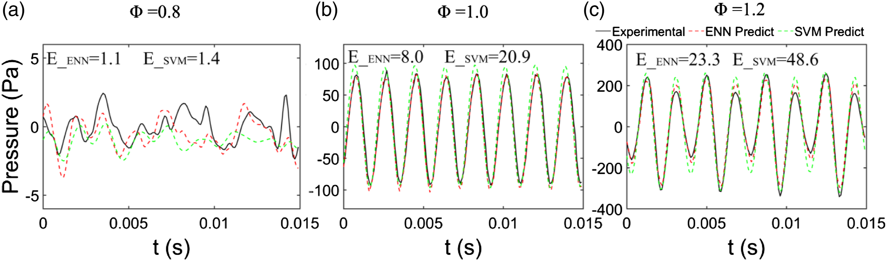

Choice of input length

The data length plays a major role in whether features can be fully extracted from the data. This means that the neural network model’s accuracy will be affected by the length of the input data. To determine the influence of different input lengths on prediction performance, a series of predictive models of different lengths were built. Training of the ENN model was performed on data with Φ = 0.9, and testing was performed on data when Φ = 1.0. The prediction performance is shown in Figure 11. First, the prediction accuracy of these models with different input lengths decreases with the increase of the predicted time horizon, which is consistent with Section. As the input length increases from L = 10 to L = 50, the $E_{R M S}$ decreases, meaning that the prediction accuracy increases with the input length. The reason for the better prediction performance may be that the model features can be fully extracted from the longer data. However, the $E_{R M S}$ no longer varies monotonically with the input length as the input length increases from 50 to 90. As can be seen, the longer length of the data does not mean the model will be more accurate, because too many input nodes may overfit the model. Considering the calculation accuracy, calculation time, and data-storage cost, we choose L = 50 as the optimal input length of the model.

Figure 11.

Influence of different input lengths on prediction performance.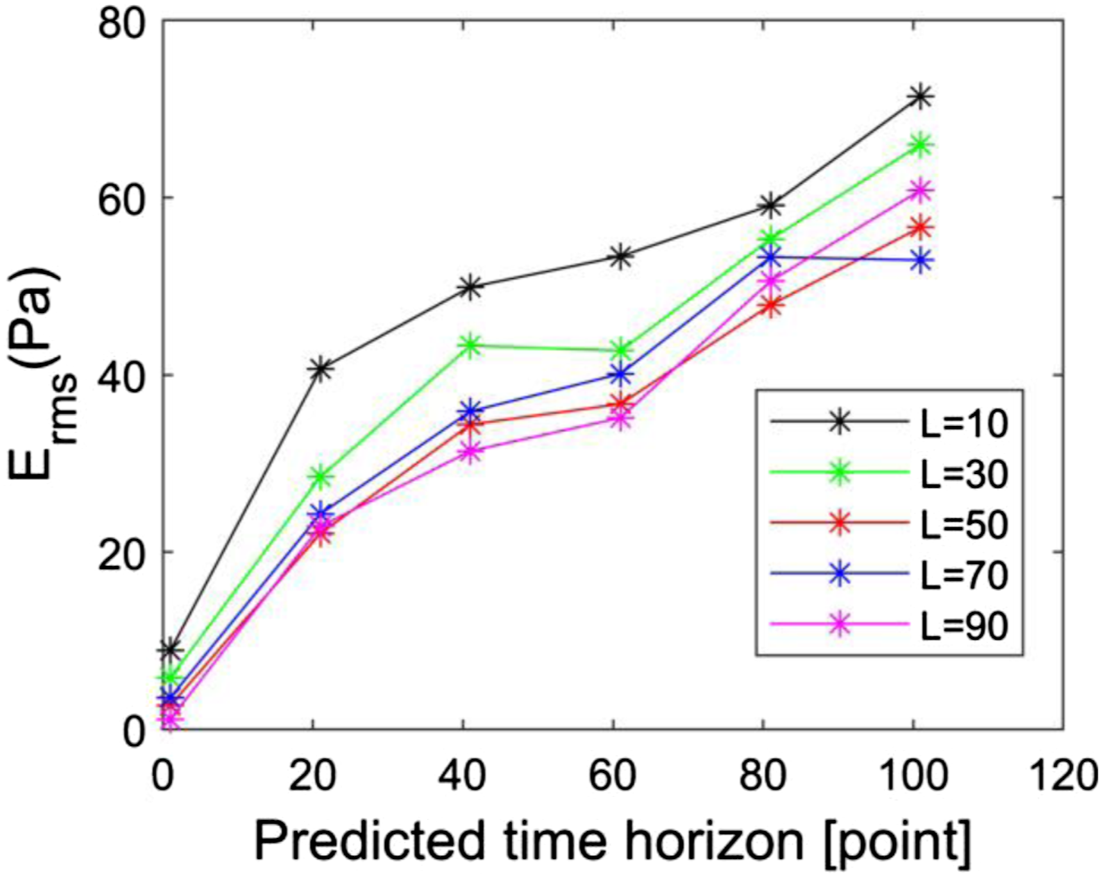

Conclusions

In this work, we systematically studied a data-driven method based on ENN to predict the acoustic pressure of thermoacoustic instability. First, through time-frequency analysis and nonlinear analysis of the acoustic pressure of the thermoacoustic system, we find that there are other types of oscillation in the thermoacoustic instability system besides the limit cycle oscillation, which proves the nonlinearity and variability of the thermoacoustic system. Then ENN is used to establish the data-driven model of the thermoacoustic instability system, which is applied to predict the value of acoustic pressure. It is demonstrated that ENN has reliable single-point performance in two oscillation modes, indicating that it has sufficient prediction accuracy and good generalization ability in combustion oscillation prediction. As for a long-term prediction, compared with SVM, ENN still has a certain ability to meet the engineering requirements for combustion stability monitoring and control. What is more, the prediction model based on ENN has the ability to adapt to time-varying characteristics of the transition scenario which is characterized by amplitude modulation, multiple frequencies, and irregular bursts. In addition, the choice of training data sets will seriously affect the prediction accuracy of SVM, but ENN can still maintain enough prediction accuracy for various oscillation types. At last, there is an optimal length of input data, and the prediction accuracy is the highest at this point.

Footnotes

Acknowledgements

The authors acknowledge the financial support from the National Science and Technology Major Project (J2019-III-0020–0064) and the National Defense Basic Scientific Research Project (JCKY2020130C025).

Declaration of conflicting interests

The author(s) declared no potential conflicts of interest with respect to the research, authorship, and/or publication of this article.

Funding

The author(s) disclosed receipt of the following financial support for the research, authorship, and/or publication of this article: This work was supported by the National Science and Technology Major Project (J2019-III-0020-0064) and the National Defense Basic Scientific Research Project (JCKY2020130C025).

ORCID iD

Qingwen Zeng

References

Zhao

, et al. A review of active control approaches in stabilizing combustion systems in aerospace industry. Prog Aeros Sci 2018; 97: 35–60, DOI: 10.1016/j.paerosci.2018.01.002

Koshigoe

Komatsuzaki

Yang

. Adaptive control of combustion instability with on-line system identification. J Prop Power 1999; 15: 383–389. Article. DOI: 10.2514/2.5456

Seume

Vortmeyer

Krause

, et al. Application of active combustion instability control to a heavy duty gas turbine. J Eng Gas Turbines Power 1998; 120: 721–726. Article. DOI: 10.1115/1.2818459

McManus

Poinsot

Candel

. A review of active control of combustion instabilities. Prog Energy Combus Sci 1993; 19: 1–29. Review. DOI: 10.1016/0360-1285(93)90020-F

Ducruix

Schuller

Durox

, et al. Combustion dynamics and instabilities: elementary coupling and driving mechanisms. J Propu Power 2003; 19: 722–734. Article. DOI: 10.2514/2.6182

Poinsot

. Prediction and control of combustion instabilities in real engines. Proc Combus Inst 2017; 36: 1–28. Article. DOI: 10.1016/j.proci.2016.05.007

Boudy

Durox

Schuller

, et al. Nonlinear flame describing function analysis of galloping limit cycles featuring chaotic states in premixed combustors. In: ASME turbo expo 2012: turbine technical conference and exposition, 2012, pp. 713–724.

Kabiraj

Saurabh

Wahi

, et al. Experimental study of thermoacoustic instability in ducted premixed flames: periodic, quasi-periodic and chaotic oscillations. In: n3l-international summer school and workshop on non-normal and nonlinear effects in aero- and thermoacoustics; Munich, 2010.

Lahiri

Bake

. A review of bias flow liners for acoustic damping in gas turbine combustors. J Sound Vib 2017; 400: 564–605. Review. DOI: 10.1016/j.jsv.2017.04.005

10.

Zhao

. A review of acoustic dampers applied to combustion chambers in aerospace industry. Prog Aeros Sci 2015; 74: 114–130. Review. DOI: 10.1016/j.paerosci.2014.12.003

11.

Zhao

, et al. Thermodynamic measurement and analysis of dual-temperature thermoacoustic oscillations for energy harvesting application. Energy 2014; 65: 517–526. Article. DOI: 10.1016/j.energy.2013.10.078.

12.

Zhao

. Feedback control of self-sustained nonlinear combustion oscillations. J Eng Gas Turb Power 2016; 138. Article. DOI: 10.1115/1.4031605

13.

Zhao

Gutmark

Reinecke

. Mitigating self-excited flame pulsating and thermoacoustic oscillations using perforated liners. Sci Bulletin 2019; 64: 941–952, DOI: 10.1016/j.scib.2019.05.004

14.

Joo

Choi

Kim

, et al. A novel diagnostic method based on filter bank theory for fast and accurate detection of thermoacoustic instability. Sci Rep 2021; 11: 3043. DOI: 10.1038/s41598-020-80427-6

15.

Waxenegger-Wilfing

Sengupta

Martin

, et al. Early detection of thermoacoustic instabilities in a cryogenic rocket thrust chamber using combustion noise features and machine learning. Chaos 2021; 31: 063128. DOI: 10.1063/5.0038817

16.

Song

Cha

. Temporal kurtosis of dynamic pressure signal as a quantitative measure of combustion instability. Appl Therm Eng 2016; 104: 577–586.

17.

Nair

Thampi

Sujith

. Intermittency route to thermoacoustic instability in turbulent combustors. J Fluid Mech 2014; 756: 470–487. 2014/09/02. DOI: 10.1017/jfm.2014.468

18.

Kasthuri

Pavithran

Pawar

, et al. Dynamical systems approach to study thermoacoustic transitions in a liquid rocket combustor. Chaos 2019; 29: 103115.

19.

Pavithran

Unni

Sujith

. Critical transitions and their early warning signals in thermoacoustic systems. Er Phy J-Special Topics 2021; 230: 3411–3432. DOI: 10.1140/epjs/s11734-021-00214-w

20.

Zhang

Huang

. Electroacoustic control of Rijke tube instability. J Sound Vib 2017; 409: 131–144. Article. DOI: 10.1016/j.jsv.2017.07.050

21.

Dhadphale

Unni

Saha

, et al. Neural ODE to model and prognose thermoacoustic instability. Chaos 2022; 32: 013131. DOI: 10.1063/5.0064215

22.

Lyu

Fang

Zhu

, et al. Prediction of acoustic pressure of the annular combustor using stacked long short-term memory network. Phy Fluids 2022; 34: 34. DOI: 10.1063/5.0089146

23.

Ruiz

Unni

Pavithran

, et al. Convolutional neural networks to predict the onset of oscillatory instabilities in turbulent systems. Chaos 2021; 31: 093131. DOI: 10.1063/5.0056032

24.

Juniper

Sujith

. Sensitivity and Nonlinearity of Thermoacoustic Oscillations. Annu Rev Fluid Mech 2018; 50: 661–689. DOI: 10.1146/annurev-fluid-122316-045125

25.

Packard

Crutchfield

Farmer

, et al. Geometry from a time series. Phy Rev Lett 1980; 45: 712–716. DOI: 10.1103/PhysRevLett.45.712

26.

Schuster

Just

. Deterministic chaos: an introduction. 4th Edition, 2005, pp. 1–287.

27.

Fraser

Swinney

. Independent coordinates for strange attractors from mutual information. Physical Review A 1986; 33: 1134–1140. DOI: 10.1103/PhysRevA.33.1134.

28.

Kennel

Brown

Abarbanel

HDI

. Determining embedding dimension for phase-space reconstruction using a geometrical construction. Physical Review A 1992; 45: 3403–3411. DOI: 10.1103/PhysRevA.45.3403.

29.

Cao

. Practical method for determining the minimum embedding dimension of a scalar time series. Physica D: Nonlinear Phenom 1997; 110: 43–50, DOI: 10.1016/S0167-2789(97)00118-8.. DOI:

. Frequency domain and time domain analysis of thermoacoustic oscillations with wave-based acoustics. J Fluid Mech 2015; 775: 387–414.

31.

Tucker Warwick . Computing accurate Poincaré maps. Physica D 2002; 171: 127–137.

32.

Elman

. Finding structure in time. Cogn Sci 1990; 14: 179–211, DOI: 10.1016/0364-0213(90)90002-E

33.

Weng