Unsupervised structural damage detection based on an improved generative adversarial network and cloud model

Abstract

The measurements derived from damaged conditions are difficult to acquire in actual structures, which limits the applicability of supervised damage detection methods. In this study, an unsupervised damage detection method that leverages an improved generative adversarial network (IGAN) and cloud model (CM) is proposed. This method only needs the data in the healthy state of the structure for model training, which can solve the above problems. Firstly, an IGAN model is established, which uses the encoder-decoder-encoder generative network to encode, reconstruct and re-encode the structural response in healthy state. The essential features hidden in complex data are learned by minimizing the distance between the real response and the reconstructed response, and the distance between the latent vectors obtained after two different encodings. During the test phase, when unknown state data is input into the model, the differences of the latent features of the two different codes can be used to preliminarily judge whether the structure is damaged. In addition, CM theory is used to further quantify structural damage and solve the problem of damage misjudgment caused by measurement noise, model parameters, feature selection, and other uncertain factors. The effectiveness of the proposed damage detection method is verified by Phase I IASC-ASCE benchmark structure and a bridge health monitoring benchmark model. The results prove that the proposed method can accurately detect the damage that has occurred.

Introduction

Under the influence of environmental erosion, loading and material aging, the service performance of civil engineering structures gradually decreases, and even collapses may occur in extreme cases, resulting in large casualties. Thus, it is necessary to recognize structural conditions in a timely manner to ensure safety. ¹ To address this problem, structural health monitoring (SHM) techniques have been increasingly proposed and applied for long-span bridges in recent decades. Actually, SHM is a procedure that aims to evaluate and predict the performance of a structure in real time via sensing techniques and structural characteristics analysis. ² As one of the core technologies of SHM systems, damage identification has been widely investigated, and many algorithms have been put forward over the past few decades. Traditional methodologies for utilizing monitoring data can be classified to model-based and data-based techniques. The former approach assumes that the given structure responds in some predetermined way that can be simulated by a numerical model. An updated model with the relevant measurements of the damaged structure is compared with the original model to identify the locations and severity of the damage.^3,4 For large and complex civil engineering structures, it is very difficult to establish accurate finite element models (FEMs) due to the influence of the structure itself or the environment. In addition to the inevitable modeling errors, the data may also be affected by improper operations or environmental factors during the measurements, leading to poor performance for model-based methods in practical applications. ⁵

Unlike model-based methods, algorithms based on data do not rely on FEMs of the input structure and can perform damage detection by directly using the collected monitoring data. This method mainly includes feature selection, feature extraction, and state classification. ⁶ Methods such as the fast Fourier transform, ⁷ empirical modal decomposition, ⁸ and wavelet transform ⁹ make sense in extracting damage-sensitive features. For feature classification, machine learning tools such as artificial neural networks, ¹⁰ support vector machines, ¹¹ and genetic algorithms ¹² have been widely used in damage detection. Unfortunately, traditional machine learning algorithms strongly depend on domain experts for feature selection, and the goodness of the obtained features directly determines the performance of the resulting algorithm. Furthermore, shallow neural networks suffer from poor generalization ability, insufficient ability to characterize complex functions, and difficulty in processing large amounts of data. ¹³

As an emerging artificial intelligence technology, deep learning can process a large amount of complex data and has the function of automatic feature extraction to avoid artificial feature extraction, thereby solving the above problems to a certain extent. At present, deep learning algorithms can be divided into supervised and unsupervised learning approaches. Supervised learning algorithms receive datasets and their corresponding labels and continuously update the network parameters through training to achieve optimality. ¹⁴ Among the techniques based on supervised deep learning, convolutional neural networks (CNN) currently have some applications in the field of structural damage identification. For example, Abdeljaber et al. ¹⁵ used the acceleration data of the healthy state and different damage states of each joint to train corresponding 1D-CNN models to locate joint damage. Lin et al. ¹³ took the wavelet packet component energy of the signals as the input feature vectors of a CNN for damage localization on a numerical beam and explained the process of performing damage feature extraction with the neural network. Zhang et al. ¹⁶ used a 1D-CNN and verified its damage detection performance on two experimental beam models and an actual bridge structure; the results showed that the network model could perfectly determine the locations of small local structural mass and stiffness changes. Guo et al. ¹⁷ designed a multiscale modular network based on a CNN to extract damage features at various scales with a consideration of different scenarios, multiple types of damage, noise interference and missing measurement data, and achieved better results. Although a structural damage identification method based on supervised learning can achieve high accuracy, it still requires a large amount of health and damage data and their corresponding labels. However, in the actual damage detection process, only the data samples generated under the condition of structural health can be obtained, and the data of structural damage state is missing.

Unlike supervised learning methods, unsupervised learning algorithms do not rely on data labels; they instead learn implicit patterns directly from the data themselves. ¹⁸ Now research on deep unsupervised damage detection is still very limited. Rafiei et al. ¹⁹ developed a deep restricted Boltzmann machine model to extract the features in denoised frequency-domain signals and used the structural health index for determining the global and local health conditions of the structural system. Ozdagli et al. ²⁰ constructed an auto-encoder (AE) network using the mode shapes and natural frequencies of the target structure and used the reconstruction error of the samples under the condition of temperature uncertainty for structural damage detection. This method either relies on manually extracted features, such as those obtained through signal processing techniques, or relies on structural modal information. Manually extracted features cannot guarantee optimality and result in the loss of effective information. The modal information is a global structural feature, which is more suitable for evaluating the overall condition of a structure. Ma et al. ²¹ learned the latent features hidden behind complex data during the encoding and decoding of high-dimensional data using a variational AE. The damage was identified by monitoring the abnormal characteristics of the data. Jiang et al. ²² proposed a decentralized end-to-end unsupervised structural condition diagnosis framework based on a deep AE and verified the method on laboratory frames and a large-scale grandstand structure. Silva et al. ²³ used a stacked AE to extract the damage-sensitive features of preprocessed vibration data for unsupervised damage detection; this approach achieved good performance on the Z-24 bridge dataset.

GAN is another type of deep learning-based unsupervised model. The framework of adversarial training, which consists of a generative model and a discriminative model, exhibits a powerful capability on pixel-to-pixel tasks such as image super-resolution, ²⁴ style translation, ²⁵ and inpainting. ²⁶ It has the ability to learn the deep features hidden behind the input data, and the generated images display clear outlines and even clear texture details. In the SHM field, GANs have been applied to various tasks, including but not limited to lost signal reconstruction, ²⁷ faulty sensor identification, ²⁸ and data augmentation for minority classes. ²⁹ Rastin et al. ³⁰ first applied this algorithm to structural damage detection and proposed a two-stage unsupervised structural damage identification method based on a deep convolutional GAN. The input of the generator in vanilla GAN is random noise, which makes it difficult to train because of the great uncertainty of this input. Akcay et al. ³¹ proposed an improved GAN for anomaly detection context of X-ray security screening. This network consists of a generator, a discriminator and an encoder. This method can solve problems mentioned above to a certain extent.

According to the published literature, although unsupervised identification can only achieve damage early warning, it is still of great significance for the realization of automation and unmanned duty function of structural health monitoring system. In this paper, an unsupervised damage detection method that leverages an IGAN and CM is proposed. An encoder-decoder-encoder network is used to encode the input vibration response into its optimal latent representation, and then the generated sample is reconstructed. An additional encoder is used to encode the generated samples, and the latent feature differences between the two encodings are used to detect structural damage. From the perspective of the latent features of signal coding, a damage quantification framework based on a CM is proposed. The training process of the model only needs the vibration acceleration signal data of the structure under normal operation, and does not need the data and labels of the damage state. The performance of the proposed algorithm is verified on a benchmark structure and a benchmark model.

The remainder of this paper is organized as follows. In unsupervised structural damage detection method based on GAN and CM section, the deep learning framework and the training and test processes of the model are introduced in detail. Case study I: Phase I IASC-ASCE SHM benchmark structure section verifies the validity of the damage detection framework on the Phase I IASC-ASCE benchmark structure. In Case study II: a bridge health monitoring benchmark model section, the damage detection capability of the proposed method considering different position sensors is verified based on the bridge health monitoring benchmark model. Finally, conclusions are drawn in final section.

Unsupervised structural damage detection method based on GAN and CM

Generative adversarial network and improved generative adversarial network

GAN is an unsupervised deep learning algorithm proposed by Goodfellow et al. ³² It was inspired by the binary zero-sum game in game theory. The vanilla GAN consists of a generative network G and a discriminative network D, as shown in Figure 1. A random noise z is defined with a prior distribution P _g and input into G, in which the generated sample G(z) obeys the true sample distribution P_data as well as possible. The inputs of D are the real sample x and the generated sample G(z), and the output result is the probability that the input is the real sample. If the discriminator thinks that the input is the real sample, it prints 1; otherwise, it prints 0. Through continuous optimization, G and D improve their generative and discriminant abilities, respectively, to find a Nash equilibrium between them. The objective function of this process can be expressed as

$\arg \underset{G}{\min }\underset{D}{\max }V\left(D,G\right)=\underset{G}{\min }\underset{D}{\max }\left[E_{x\sim P_{\mathrm{d}\mathrm{a}\mathrm{t}\mathrm{a}}}\left(logD\left(x\right)\right)+E_{z\sim P_g}\left(\log (1-D\left(G\left(z\right)\right))\right)\right]$

(1)

Figure 1.

General form of a GAN.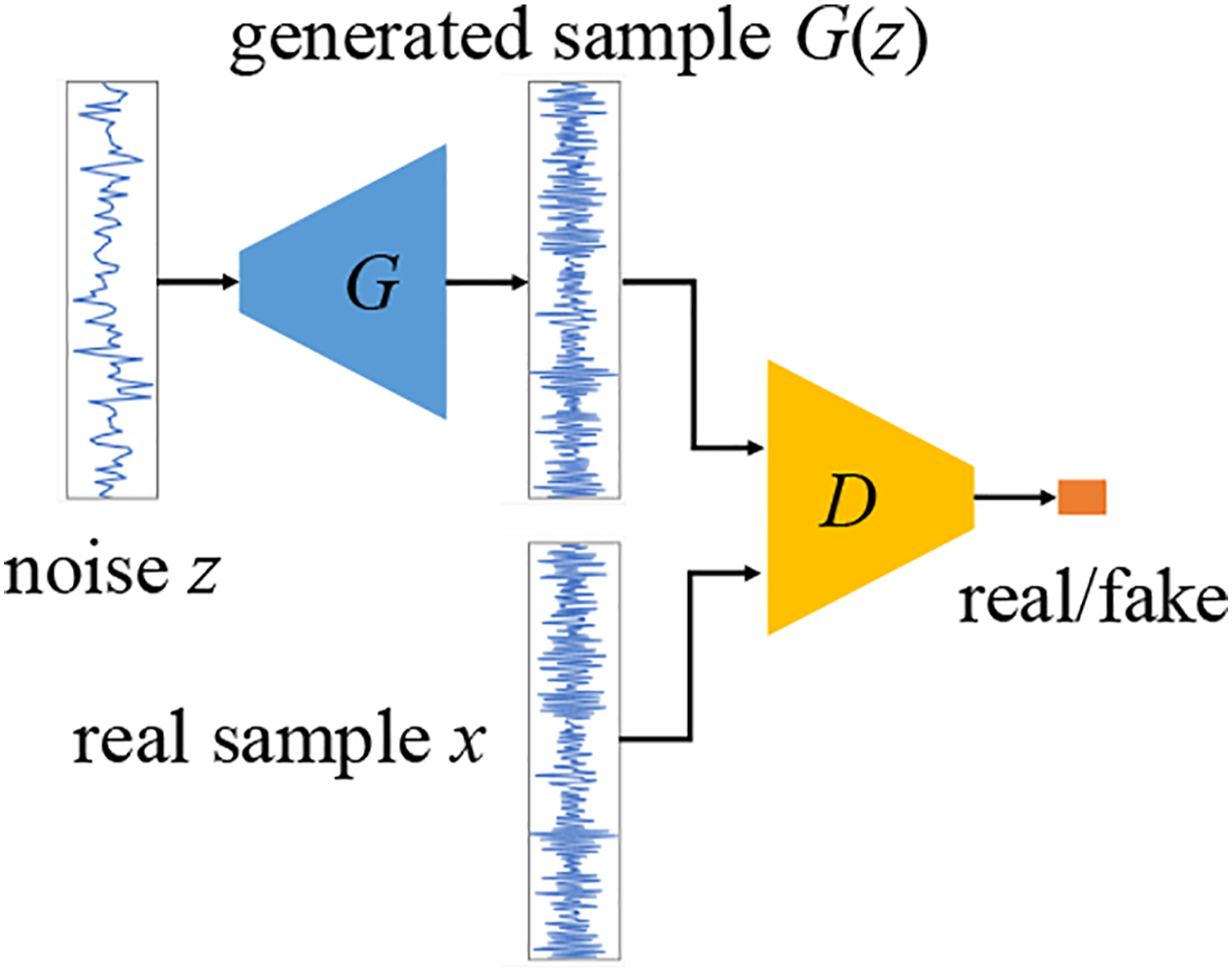

The input of the generator in vanilla GAN is random noise, which makes it difficult to train because of the great uncertainty of this input. Figure 2 shows an overview of the IGAN used in this paper, originally used by Akcay et al. ³¹ for anomaly detection context of X-ray security screening. The network consists of a generator, a discriminator and an encoder. The generator is designed as a deep convolutional encoder–decoder pipeline. The inputs of the generator are normal samples, thereby ensuring the consistency of the input data so that the training difficulty is reduced. The generation network and the discrimination network play games with each other, and the sample generation capability of the decoder and the feature extraction capability of the encoder are improved. The latent feature z of the input sample x can better reflect the effective information of the input sample, and the interference induced by noise and other vibration components on the detection result is reduced. During the training process, the real sample is input into G, and x is compressed to a bottleneck layer of dimension z through multiple convolution layers, batch normalization (BN) layers and activation function layers in the encoder. z is the best representation of x and contains the latent high-level features of x. The decoder G _D in G uses multiple transposed convolution layers, BN layers and activation function layers to reconstruct the vector z as G(x). 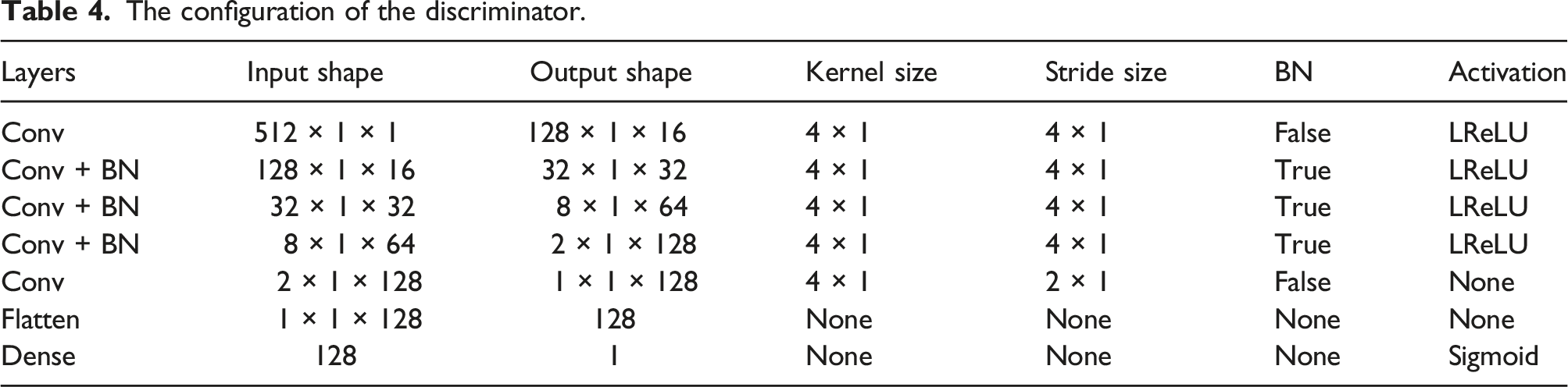The second encoder E, which has the same network architecture as G _E , encodes the G(x) reconstructed by G and compresses it into the vector z′, which has the same dimensionality as z. The front part of the discriminant network D is also an encoder in which x and G(x) are input and encoded, and finally, the output value is mapped to [0,1] through the sigmoid activation function in the output layer.

Figure 2.

The architecture of the improved GAN.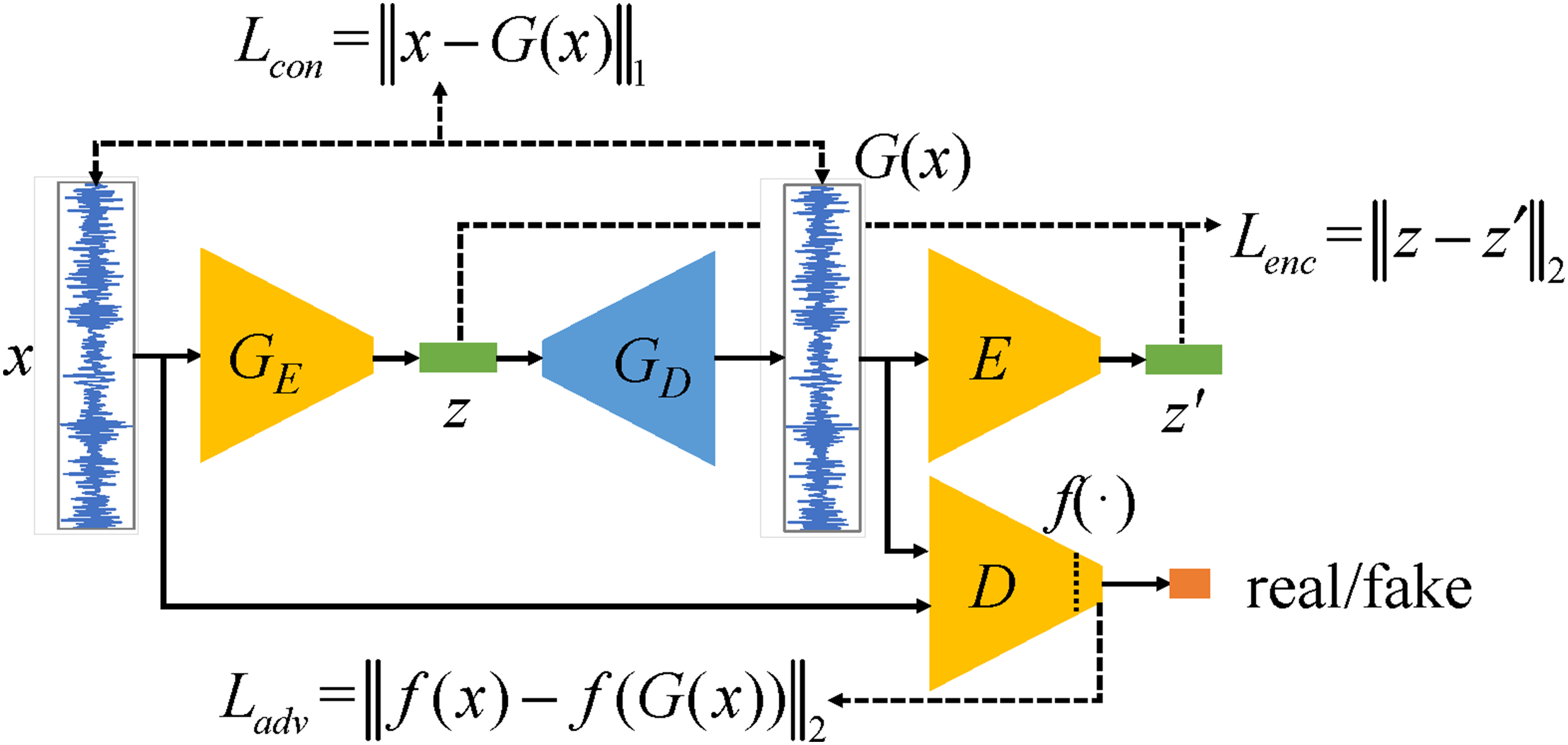

Unsupervised structural damage detection method based IGAN and CM

The IGAN and CM are utilized for damage detection in this paper. The flow of the proposed unsupervised structural damage detection method in this paper is shown in Figure 3. Firstly, the required acceleration signals are collected on an SHM system. The processed health data are used as the training set, and a portion of the healthy data and all damage data are used as the test set. The deep learning network structure of the proposed algorithm is trained using the training set, and damage detection is performed on the test set samples based on the feature differences observed after secondary encoding. Finally, the CMs for damage quantification are established.

Figure 3.

The pipeline of the proposed approach for damage detection.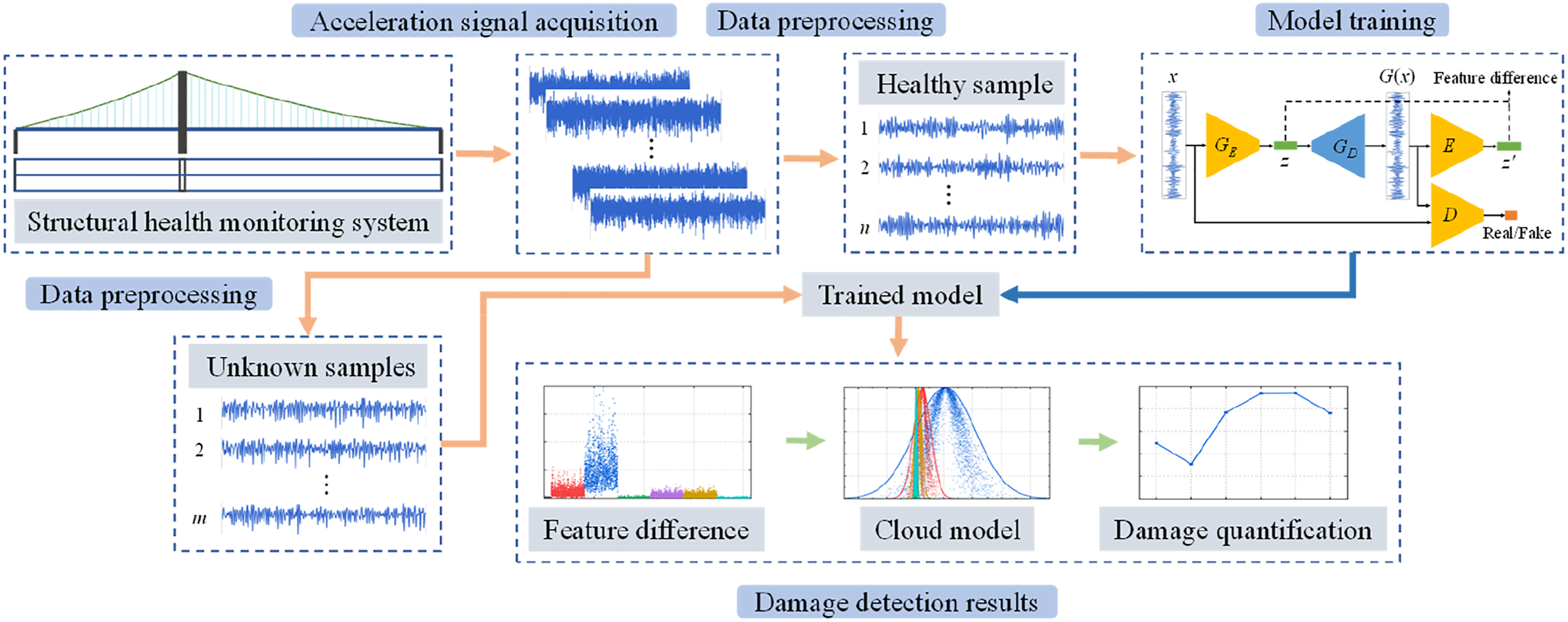

Training phase

During the operation process of the SHM system, data for the normal state of the structure are easy to collect. Before training the deep learning model, the collected data need to be preprocessed to convert the original data into a format that can be understood by the neural network. A schematic of the preprocessing method is shown in Figure 4, which mainly includes data normalization and data slicing. Because the measured signals have different fluctuation ranges, the normalization method is used to transfer them to the same scale, and the normalization range is [−1, 1]. To adapt to the input size of the network, the normalized signals must be sliced. To obtain more training samples, a window with a length of 512 and a step size of 50 is used to slide along the time steps of the acceleration data. This requires only 50 additional data points for each additional sample generated. The length of each sample after preprocessing is 512.

Figure 4.

Data preprocessing.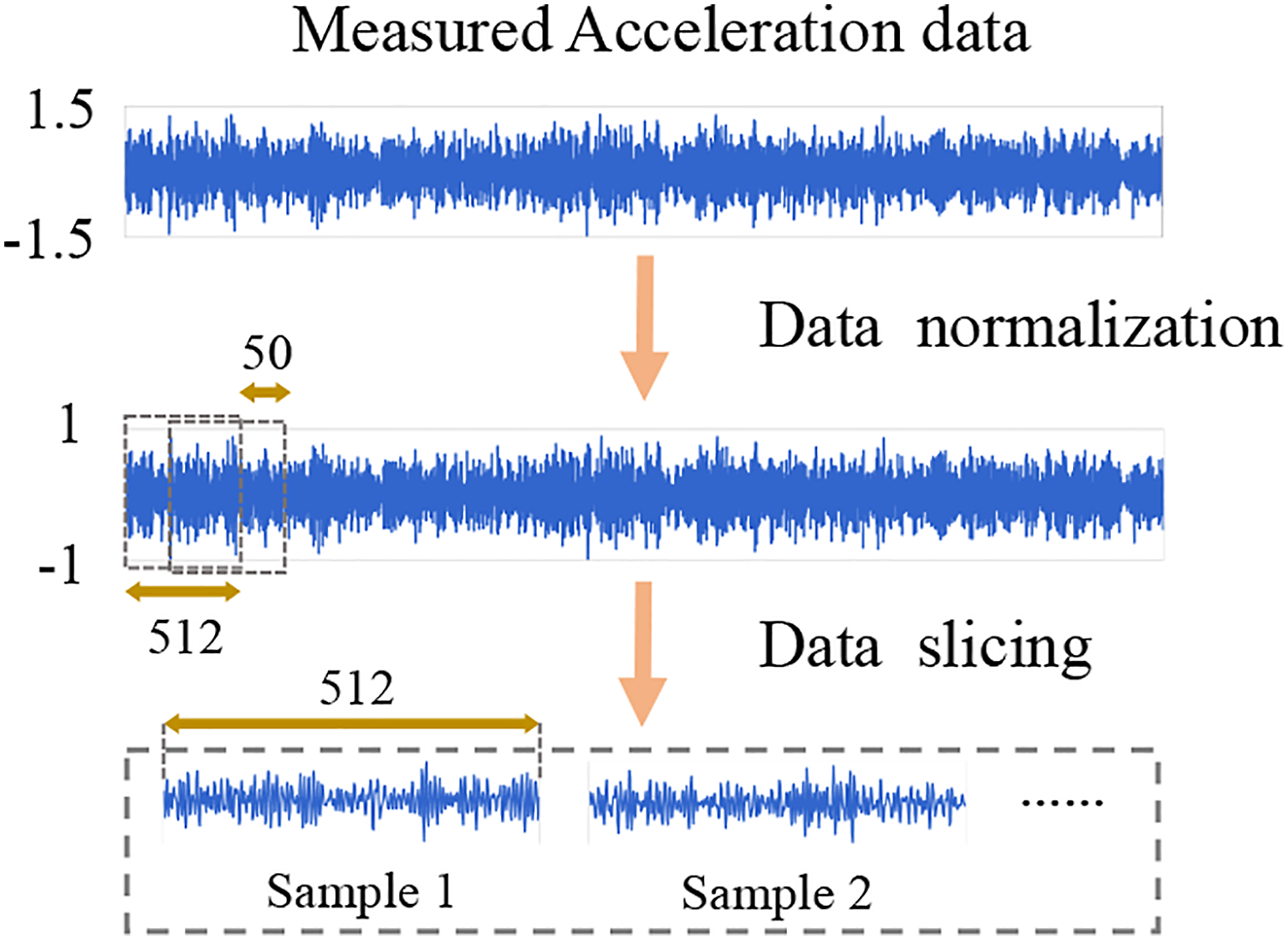

During the training phase, the preprocessed sample is input into the generator, and the first sub-network G _E in the generator encodes the sample to obtain the latent feature z. The decoder G _D then decodes z to obtain the generated sample G(x). To make the data distribution of G(x) as close as possible to that of x, the L₁ loss is used to optimize the objective function L _con

$L_{con}=\min E_{x\sim p_{\text{data}}}{\Vert x-G\left(x\right)\Vert }_1,$

(2)

To obtain the differences among latent features, the generated sample is encoded by the encoder E to obtain a latent encoding z′. The feature z and the distribution of the feature z′ in the latent space are optimized by an additional encoder loss L _enc . The objective function L _enc is

$L_{enc}=\min E_{x\sim p_{\text{data}}}{\Vert G_E\left(x\right)-E\left(G\left(x\right)\right)\Vert }_2,$

(3)

Subsequently, the real sample and the generated sample are input into the discriminator network. To reduce the instability of the GAN training process, the feature matching loss is used for adversarial learning. ³³ f is the output function of an intermediate layer of D, and feature matching calculates the L₂ distance between the feature representation of the real sample and that of the reconstructed sample. Thus, the adversarial loss L _adv is defined as

$L_{adv}=\min E_{x\sim p_{\text{data}}}{\Vert f\left(x\right)-E_{x\sim p_{\text{data}}}f\left(G\left(x\right)\right)\Vert }_2,$

(4)

Overall, the objective function for the generator becomes the following

$L=w_{con}{L}_{con}+w_{adv}{L}_{adv}+w_{enc}{L}_{enc},$

(5)

where w _con = 1, w _adv = 40 and w _enc = 1.

The objective function is formulated by combining three loss functions, each of which optimizes a single sub-network. ³¹

Test phase

During the test phase, the health samples of the test set are first input into the trained model. The latent feature z was obtained by entering the test sample x with G _E code, and then the latent feature z′ was obtained by G _D and E, from which the difference between z and z′ could be calculated, and the latent feature differences of the healthy samples were taken as the baseline. Then, the sample of unknown state is input into the model, and the damage of the structure is detected by comparing its latent feature difference with the baseline. When the sample of unknown state is the damage sample, the latent feature difference will be larger than the baseline, and the greater the damage, the further the deviation from the baseline.

Damage detection mechanism

The data acquisition process is affected by uncertainty factors such as measurement noise and sensor accuracy. A certain degree of randomness is also present in the division of the dataset and the selection of features by the network; this is manifested by the fact that each time the same network is run, different results are obtained. To effectively address the randomness and fuzziness of uncertainty, this paper adopts the similarity measure of the CM ³⁴ to measure the similarity between the latent feature differences distributions of each damage state and the healthy state and then effectively distinguishes the degree of the structural damage. The specific calculation process is described as follows.

The CM is a cognitive qualitative and quantitative transformation model composed of several cloud droplets. Cloud droplets are random realizations of a qualitative concept, and cloud drops that are generated repeatedly can comprehensively reflect the overall characteristics of this qualitative concept. ³⁴ C (Ex, En, He) represents the numerical characteristics of the cloud through the three parameters of the CM: the expected value (Ex), entropy (En), and hyper entropy (He). Ex represents the basic deterministic domain of the qualitative concept, En represents the uncertainty of the qualitative concept, and He represents the uncertainty of entropy. The expectation curve and maximum boundary curve of a normal cloud with an analytical formula can easily and effectively describe the overall characteristics of this normal cloud. Therefore, the similarity can be measured by solving the overlapping area between the expectation curve and maximum boundary curve of the two CMs, as shown in Figure 5. The similarity measure can be divided into an expectation based on the CM (ECM) and a maximum boundary based on the CM (MCM). ³⁵ This paper mainly adopts the MCM to construct the structural damage indicator.

Figure 5.

Two CM similarity calculation methods (a). ECM (b). MCM.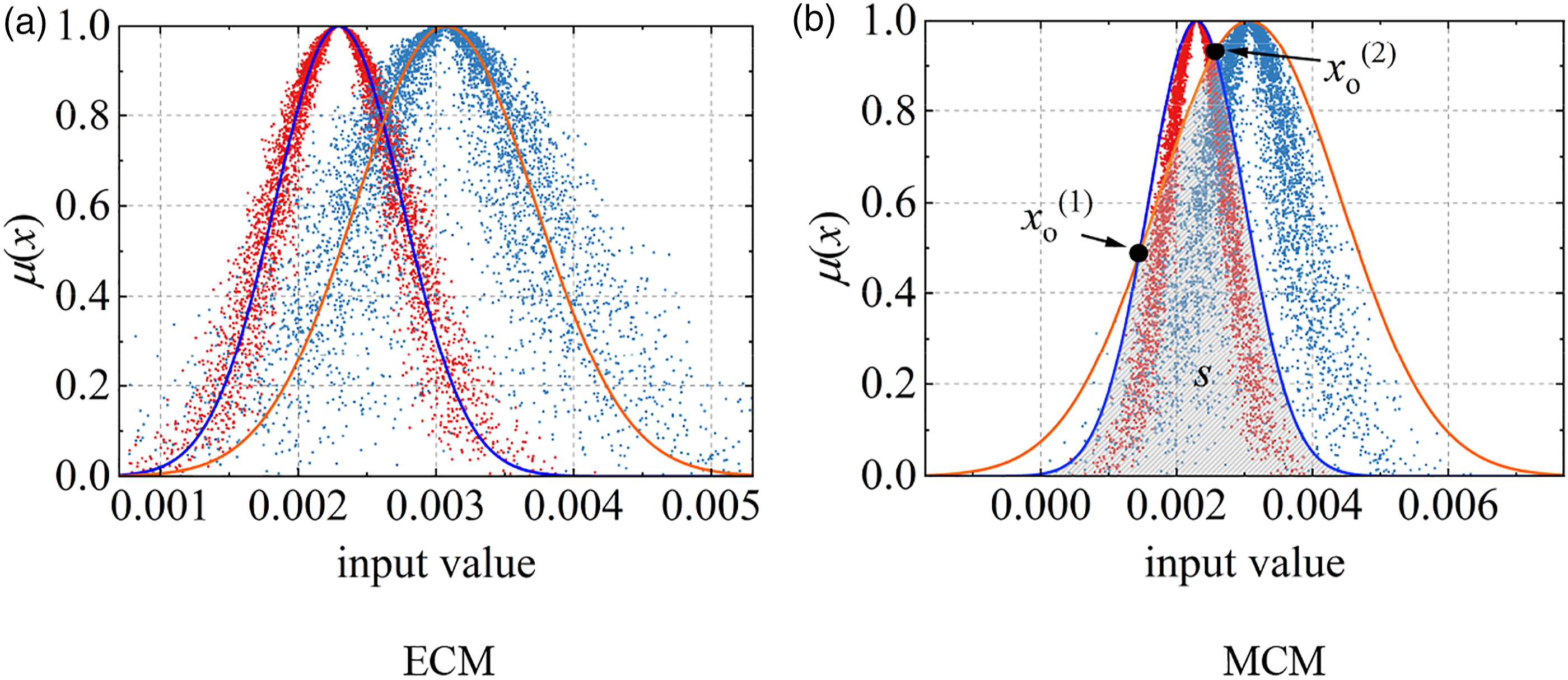

Many phenomena in the real world obey or nearly obey normal distributions, so they have certain universality. Before the MCM is used for similarity measurement, it is assumed that the distribution of the latent feature difference x in each state is a normal distribution. x obeys a normal distribution with a mathematical expectation of Ex and a variance of En′²; this distribution is denoted as N (Ex, En′²), where En’ ∼ N (En, He²). The expression of the maximum boundary curve of the CM is expressed as follows

$y=e^{-\frac{{\left(x-Ex\right)}^2}{2{\left(3He+En\right)}^2}},$

(6)

The distribution of the latent feature differences with the healthy state is set as C₁ (Ex₁, En₁, He₁), and the distribution the of latent feature differences for an unknown state is set as C₂ (Ex₂, En₂, He₂). By standardizing the overlapping area S between the maximum boundary curves of two CMs, C₁ and C₂, the MCM similarity S^MCM can be obtained, namely, the following structural damage indicator

$S^{\mathrm{M}\mathrm{C}\mathrm{M}}\left(C_1, C_2\right)=\frac{2S}{\sqrt{2}\pi \left(3H{e}_1+E{n}_1+3H{e}_2+E{n}_2\right)},$

(7)

where $\sqrt{2}\pi$ (3He₁+En₁) and $\sqrt{2}\pi$ (3He₂+En₂) represent the areas formed between the maximum boundary curves of C₁ and C₂ and the abscissa, respectively.

Due to the distribution property of the Gaussian distribution, 99.7% of cloud drops fall into the interval [Ex-3En, Ex+3En]. This means that the drops out of this interval can be ignored. When calculating the overlapping area S, we only need to consider the area on the interval [Ex-3En, Ex+3En]. Firstly, two different intersections ${x_{\mathrm{o}}}^{\left(1\right)}$ and ${x_{\mathrm{o}}}^{\left(2\right)}$ of the maximum boundary curves of C₁ and C₂ are calculated. According to the relationship between the two intersections and the 3En interval, three cases can occur: (1) the two intersections are not in the 3En interval, and the overlapping area between the two CMs is 0; (2) only one of the two intersection points is within the 3En interval; (3) both intersections are within the 3En interval. According to the different situations regarding the two intersections, the specific calculation method for the overlapping area S is referred to Li et al. ³⁵

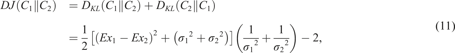
As the value range of the S^MCM is [0,1], when the damage degree is greater than a certain level, the overlapping area between the maximum boundary curves of the two CMs is 0, and the S^MCM is always 0. In this case, the degree of structural damage cannot be accurately measured. To this end, the concept of Kullback–Leibler divergence (KLD) is introduced on the basis of the MCM to better quantify severe structural damage.^36,37 For two CMs, C₁ and C₂, the KLD is defined as follows

$D_{KL}\left(C_1\Vert C_2\right)=\int c_1\left(x\right)\log \frac{c_1\left(x\right)}{c_2\left(x\right)}dx,$

(8)

where c₁(x) and c₂(x) are the density functions of two CMs C₁ and C_2, respectively.

For these CMs, directly calculating D _KL (C₁‖C₂) with its probability density function may lead to the absence of an analytical solution. Therefore, the difference between the two CMs is measured by calculating the difference between their maximum boundary curves. The maximum boundary curves of the two CMs are y₁(x) and y₂(x), and the probability density functions of their corresponding distributions are as follows

$c_1\left(x\right)=\frac{1}{\sqrt{2\pi }\left(E{n}_1+3H{e}_1\right)}{y}_1\left(x\right),$

(9)

$c_2\left(x\right)=\frac{1}{\sqrt{2\pi }\left(E{n}_2+3H{e}_2\right)}{y}_2\left(x\right),$

(10)

Equation (8) does not exhibit non-negativity and symmetry, which is inconsistent with the actual situation, so it is transformed

$\begin{array}{l}DJ\left(C_1\Vert C_2\right)=D_{KL}\left(C_1\Vert C_2\right)+D_{KL}\left(C_2\Vert C_1\right)\\ =\frac{1}{2}\left[{\left(E{x}_1-E{x}_2\right)}^2+\left({{\sigma }_1}^2+{{\sigma }_2}^2\right)\right]\left(\frac{1}{{{\sigma }_1}^2}+\frac{1}{{{\sigma }_2}^2}\right)-2,\end{array}$

(11)

where ${\sigma }_1$ = En₁+3He₁ and ${\sigma }_2$ = En₂+3He₂. A larger DJ (C₁‖C₂) indicates greater variability between C₁ and C₂.

Case study I: Phase I IASC-ASCE SHM benchmark structure

Data preparation

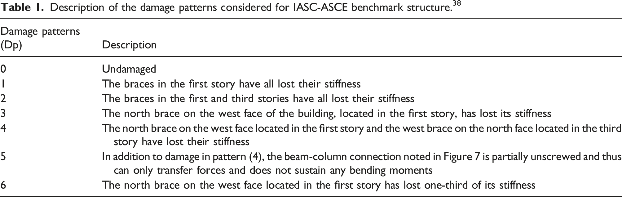
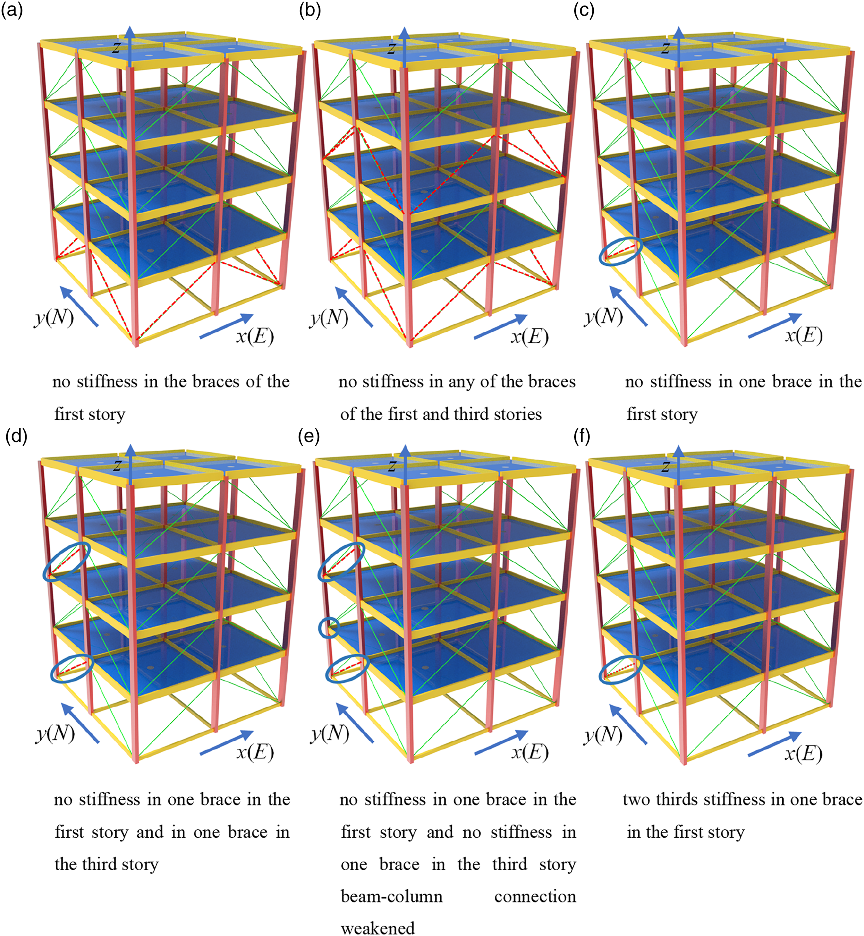
Phase I SHM benchmark structure was established by the International Association Structural Control (IASC)-American Society of Civil Engineers (ASCE) Structural Health Monitoring Task Group to provide uniform test cases for consistent evaluation of the proposed SHM methods. ³⁸ Data from a finite element model of a laboratory scale-model structure developed by the Task Group, were used in this study. The structural model shown in Figure 6, is a four-story, two-bay by two-bay steel-frame quarter-scale model structure in the Earthquake Engineering Research Laboratory at the University of British Columbia. It has a 2.5 m × 2.5 m plan and is 3.6 m tall. On each floor of each exterior face, there are two diagonal braces that may be removed to emulate damage. There is one floor slab per bay per floor. Two finite element models with 12 degrees of freedom (DOF) and 120-DOF were developed based on the structure to generate simulated response data. In both finite element models, the column and floor beams are modeled as Euler-Bernoulli beams. The braces are bars with no bending stiffness. In this paper, the 120-DOF model is used, which only requires the floor nodes to have the same horizontal translation and in-plane rotation. In addition to the undamaged structure, six damage patterns were studied. The specific description and illustrations of these damage patterns are shown in Table 1 and Figure 7.

Figure 6.

Diagram of IASC-ASCE benchmark structure. ³⁸ (a) No stiffness in the braces of the first stor. (b) No stiffness in any of the braces of the first and third stories. (c) No stiffness in one brace in the first story. (d) No stiffness in one brace in the first story and in one brace in the third story. (e) No stiffness in one brace in the first story and no stiffness in one brace in the third story beam-column connection weakened. (f) Two thirds stiffness in one brace in the first story.

Table 1.

Description of the damage patterns considered for IASC-ASCE benchmark structure. ³⁸

Damage patterns (Dp)	Description
0	Undamaged
1	The braces in the first story have all lost their stiffness
2	The braces in the first and third stories have all lost their stiffness
3	The north brace on the west face of the building, located in the first story, has lost its stiffness
4	The north brace on the west face located in the first story and the west brace on the north face located in the third story have lost their stiffness
5	In addition to damage in pattern (4), the beam-column connection noted in Figure 7 is partially unscrewed and thus can only transfer forces and does not sustain any bending moments
6	The north brace on the west face located in the first story has lost one-third of its stiffness

Figure 7.

The six damage patterns considered for the IASC-ASCE benchmark structure. ³⁸

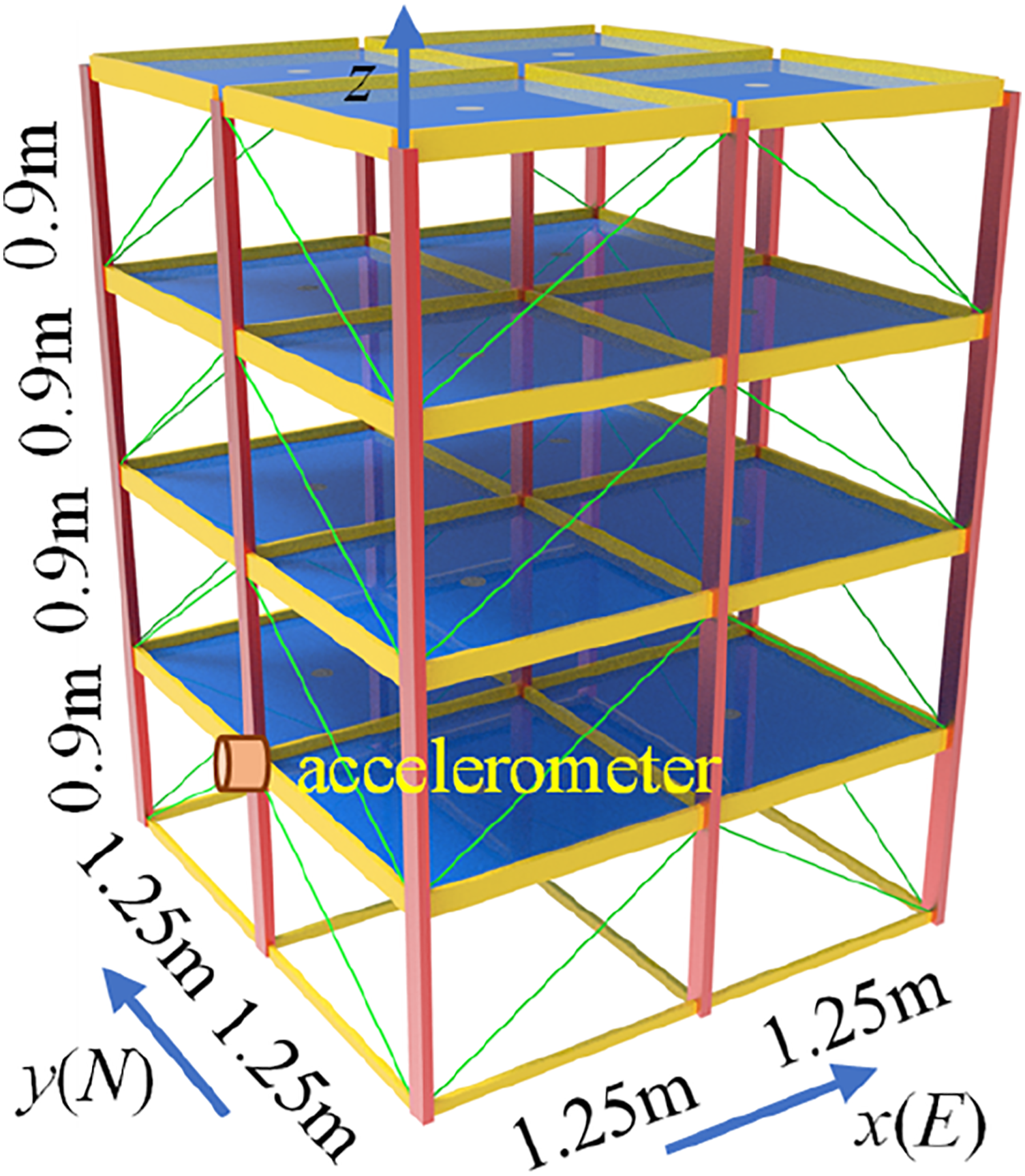
In this study, the vibration acceleration data collected by an accelerometer given in Figure 6 are used. The excitation mode is diagonal vibration of the top layer, the sampling frequency is 250 Hz, and the acquisition time of each working condition is 402 s. The size of the data set obtained is 7 × 402 × 250, and the data processing method mentioned in data preparation section is used to preprocess the data set. The total number of samples obtained by the preprocessed is 14,000, of which 80% of the healthy samples (1600) are used as the training set, and the remaining 20% of the healthy samples (400) and all the damage samples (12,000) are used as the test set. Four different levels of white Gaussian noise (5%, 10%, 15%, and 20%) were added to the acceleration data to verify the noise immunity of the model.

Network configurations

The detailed configurations of the encoder, the decoder and the discriminator are listed in Tables 2–4, respectively. The network configuration of decoder G _D is symmetrical with that of encoder G _E . The network configurations of encoders G _E and E and the feature extraction part of the discriminator are the same. Since each signal is normalized to [−1,1], the activation function of the output layer of the decoder is set to Tanh. The hidden layer in the encoder uses the leaky rectified linear unit (LReLU) as the activation function, and the activation function in the decoder is the ReLU. The discriminator aims to determine the authenticity of the generated data and uses the Sigmoid function as the activation function of the output layer. The proposed method is implemented in Keras using the Adam optimization network with an initial learning rate lr = 0.0002, and momentums β₁ = 0.5, β₂ = 0.999.

Table 2.

The configuration of the encoder.

Layers	Input shape	Output shape	Kernel size	Stride size	BN	Activation
Conv	512 × 1 × 1	128 × 1 × 16	4 × 1	4 × 1	False	LReLU
Conv + BN	128 × 1 × 16	32 × 1 × 32	4 × 1	4 × 1	True	LReLU
Conv + BN	32 × 1 × 32	8 × 1 × 64	4 × 1	4 × 1	True	LReLU
Conv + BN	8 × 1 × 64	2 × 1 × 128	4 × 1	4 × 1	True	LReLU
Conv	2 × 1 × 128	1 × 1 × 128	4 × 1	2 × 1	False	None

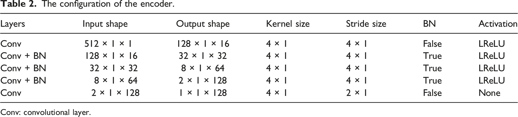
Conv: convolutional layer.

Table 3.

The configuration of the decoder.

Layers	Input shape	Output shape	Kernel size	Stride size	BN	Activation
UConv + BN	1 × 1 × 128	2 × 1 × 128	4 × 1	2 × 1	True	ReLU
UConv + BN	2 × 1 × 128	8 × 1 × 64	4 × 1	4 × 1	True	ReLU
UConv + BN	8 × 1 × 64	32 × 1 × 32	4 × 1	4 × 1	True	ReLU
UConv + BN	32 × 1 × 32	128 × 1 × 16	4 × 1	4 × 1	True	ReLU
UConv	128 × 1 × 16	512 × 1 × 1	4 × 1	4 × 1	False	Tanh

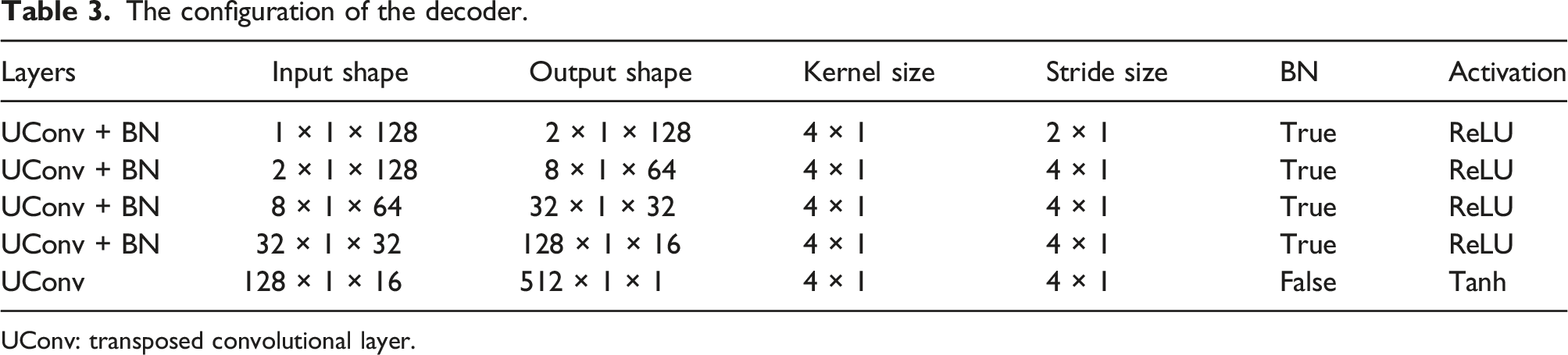
UConv: transposed convolutional layer.

Table 4.

The configuration of the discriminator.

Layers	Input shape	Output shape	Kernel size	Stride size	BN	Activation
Conv	512 × 1 × 1	128 × 1 × 16	4 × 1	4 × 1	False	LReLU
Conv + BN	128 × 1 × 16	32 × 1 × 32	4 × 1	4 × 1	True	LReLU
Conv + BN	32 × 1 × 32	8 × 1 × 64	4 × 1	4 × 1	True	LReLU
Conv + BN	8 × 1 × 64	2 × 1 × 128	4 × 1	4 × 1	True	LReLU
Conv	2 × 1 × 128	1 × 1 × 128	4 × 1	2 × 1	False	None
Flatten	1 × 1 × 128	128	None	None	None	None
Dense	128	1	None	None	None	Sigmoid

The latent feature z is the critical parameter in the network, which has a great influence on the training results. To find its appropriate size, the area under the curve (AUC) based on the Receiver Operating Characteristic (ROC) is used to compare the training results of models with different sizes of the latent feature z. The process is shown in Figure 8. The test set contained part of healthy samples and a large number of samples with different damage patterns. The trained model was used to test the test set, and the mean square error (MSE) of the two latent features obtained by twice encoding of all samples in the test set was obtained, and then the latent feature differences was normalized to [0,1]. The healthy samples in the test set were regarded as positive samples and the injured samples as negative samples. By setting different thresholds, true positive rate (TPR) and false positive rate (FPR) are calculated, as shown in equations (12) and (13)

$\mathrm{T}\mathrm{P}\mathrm{R}=\frac{\mathrm{T}\mathrm{P}}{\mathrm{T}\mathrm{P}+\mathrm{F}\mathrm{N}},$

(12)

$\mathrm{F}\mathrm{P}\mathrm{R}=\frac{\mathrm{F}\mathrm{P}}{\mathrm{F}\mathrm{P}+\mathrm{T}\mathrm{N}},$

(13)

where true positive (TP) denotes the positive samples are predicted to be the positive samples; false negative (FN) denotes the positive samples are predicted to be the negative samples; false positive (FP) denotes the negative samples are predicted to be the positive samples; true negative (TN) denotes the negative samples are predicted to be the negative samples.

Figure 8.

The process of calculating AUC.

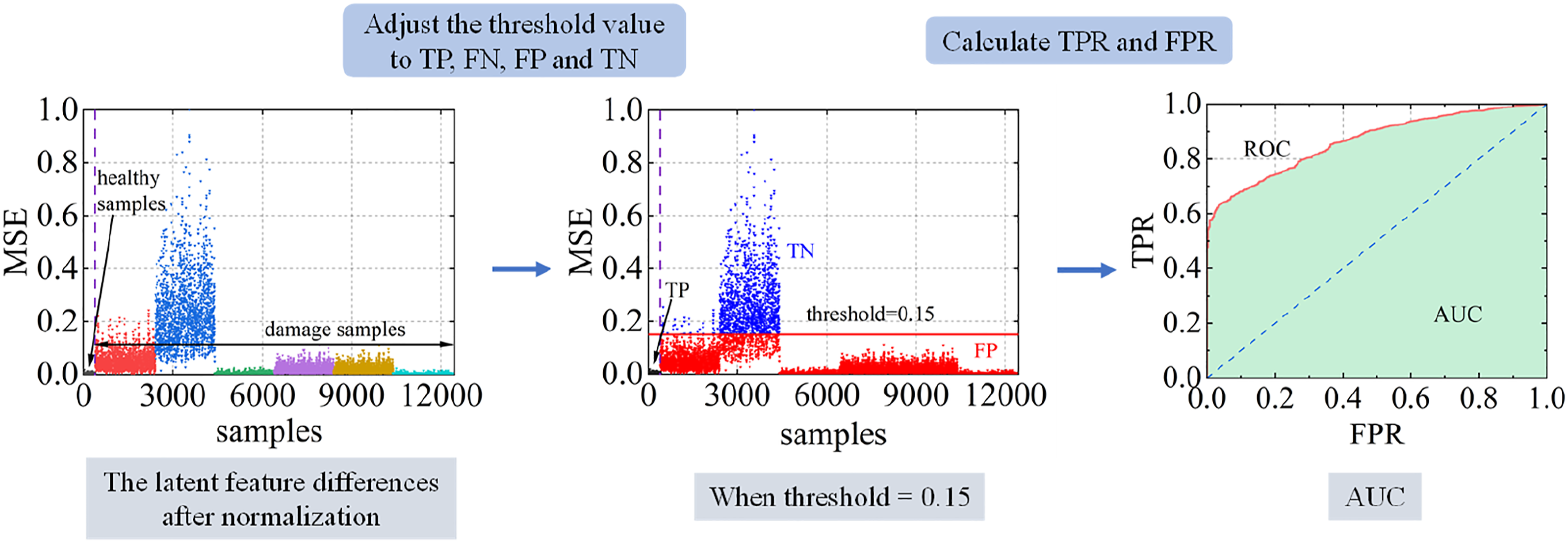
When the threshold is 0.15, as shown in Figure 8. By setting the threshold to [0,1], multiple TPR and FPR were obtained, and finally AUC was obtained according to the ROC curve. The AUC with different latent feature size z is shown in Figure 9. When the size of latent feature z is 128, the model has the best performance.

Figure 9.

Overall performance of the model based on varying size of the latent feature z.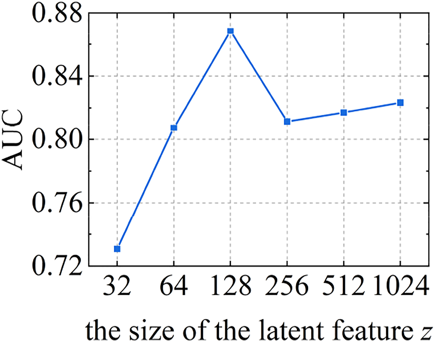

Results

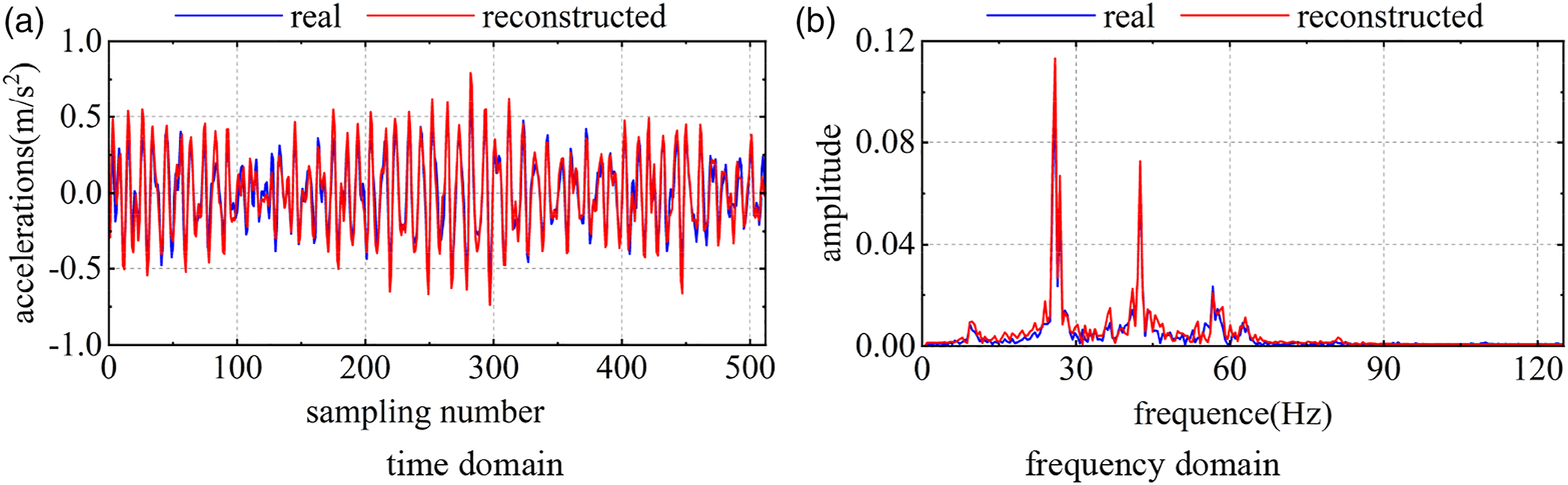
Figure 10 shows the training process of network for 500 epochs. As the network parameters are updated iteratively, the value of the objective function gradually decreases, and the loss function reaches the minimum value of 1.876 at the 463th iteration. Figure 11 shows the reconstruction effects obtained for a healthy sample in the test set in the time domain and frequency domain. The reconstructed signal is close to the true value in both the time domain and frequency domain, and the reconstruction error (MSE) is only 0.008, which indicates that the model has learned how to reconstruct the healthy samples.

Figure 10.

Change curve of the objective function value versus the number of iterations.

Figure 11.

Comparison between real and generated signals in the time domain and frequency domain. (a) time domain (b) frequency domain.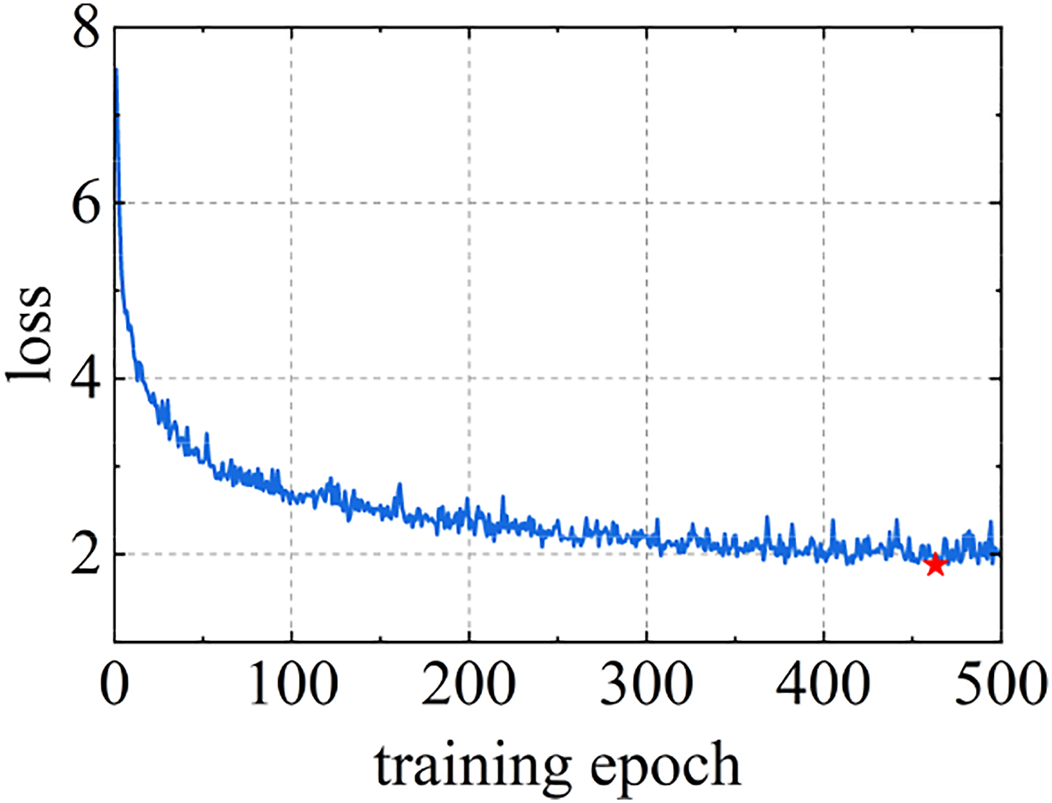

The test set contains data with structures in different states. During the test phase, data from known health states are first fed into the training model to calculate its latent feature differences and serve as a baseline. Then the samples of other unknown states are input into the model to obtain their latent feature differences. The scatter diagram of MSE values for latent feature differences of each test sample is shown in Figure 12. In order to facilitate the observation and understanding of the damage detection results of the algorithm, the damage modes of the test samples are marked in Figure 12. As can be seen from Figure 12, the latent feature differences of test samples in healthy state are very small, while the MSE value of test samples in other damaged states is large, and the MSE value increases gradually with the increase of damage degree. The identification results of each test sample under the same damage state have certain discreteness. Figure 13 shows the distribution of the latent feature differences in the test set for four different noise levels. With the increase of noise level, the latent feature differences of the damaged samples decrease, and the gap between the damaged samples and the healthy samples decreases. This shows that noise has a certain effect on the extraction of damage features.

Figure 12.

Distributions of latent feature differences in the test set at 0% noise level. (a) 5% noise level (b) 10% noise level (c) 15% noise level (d) 20% noise level.

Figure 13.

Distributions of latent feature differences in the test set.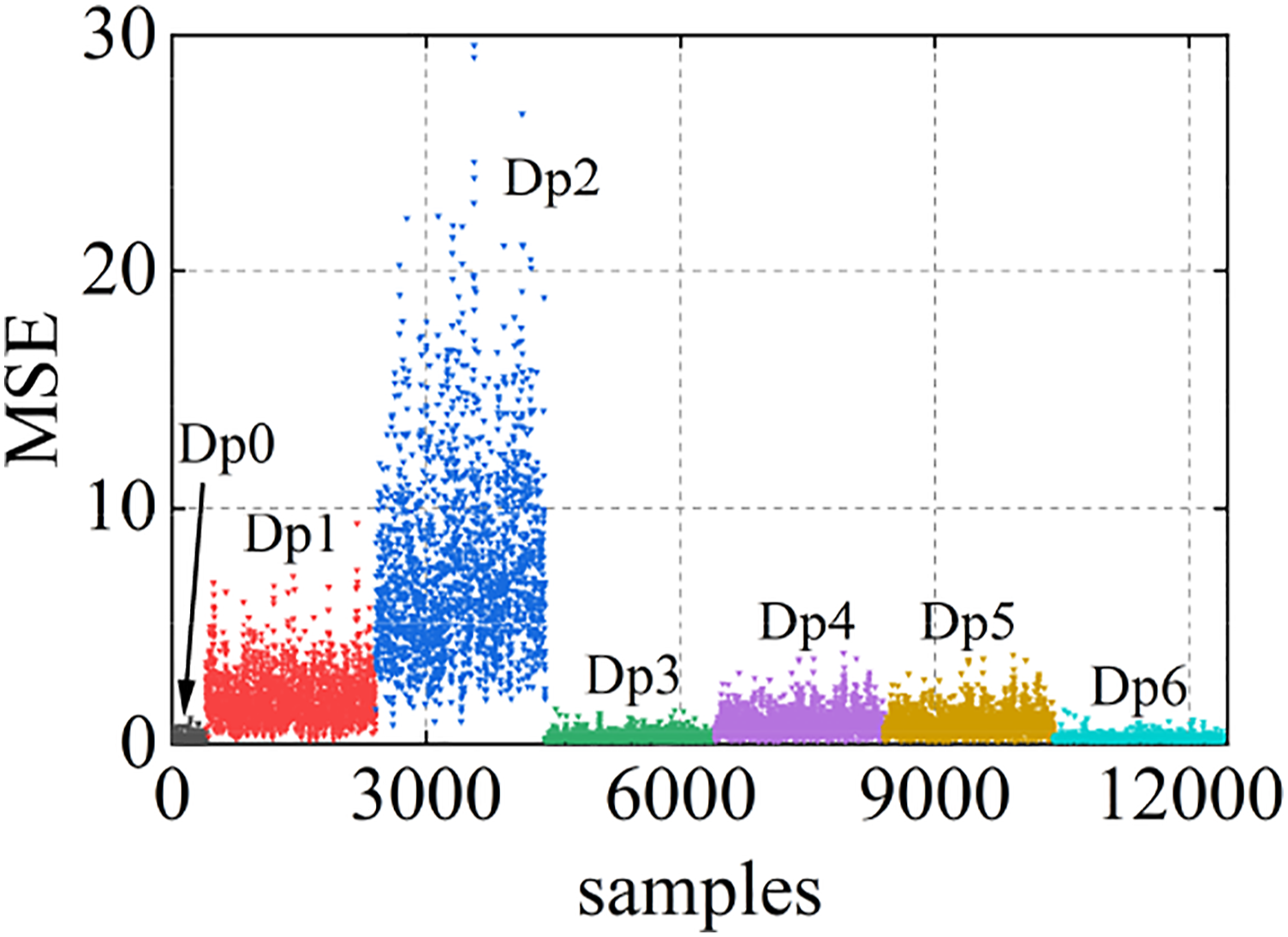

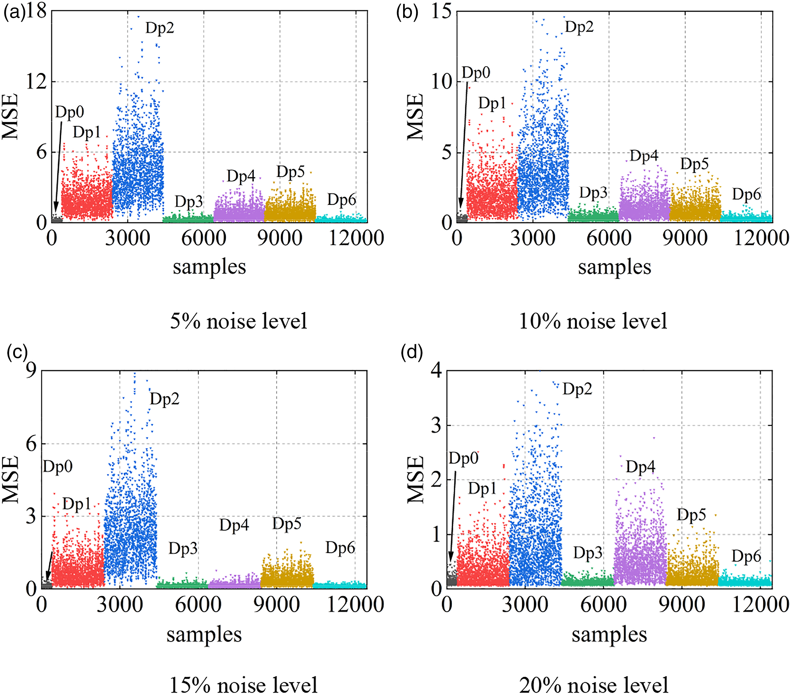
It can be seen from Figures 12 and 13 that the difference between the latent feature difference of the test sample and that of the healthy sample can be used to preliminarily determine whether the structure is damaged. Considering that the identification of different test samples under the same state has certain discreteness, CM can be used to measure the difference between multiple test results in unknown state and those in healthy state, so as to better judge whether there is damage to the structure. The comparison of CM maximum boundary curves based on the latent feature differences between each damage state and health state at 0% noise level is shown in Figure 14, from which the hierarchical relationship between different damage states can be clearly seen. The MCM of the latent feature differences between healthy samples in the test set was used as the reference baseline. With the increase of damage degree, the distribution center gradually shifts to the right side, and the distribution becomes more discrete. Dp3 and Dp6 shows the little damage, and the curve almost coincides with the healthy state. The distribution of Dp2 is the most discrete, the curve deviates the farthest from the healthy state, and the degree of damage is the largest.

Figure 14.

MCMs comparison of healthy health and all damage modes at 0% noise level. (a) Dp1 (b) Dp2 (c) Dp3 (d) Dp4 (e) Dp5 (f) Dp6.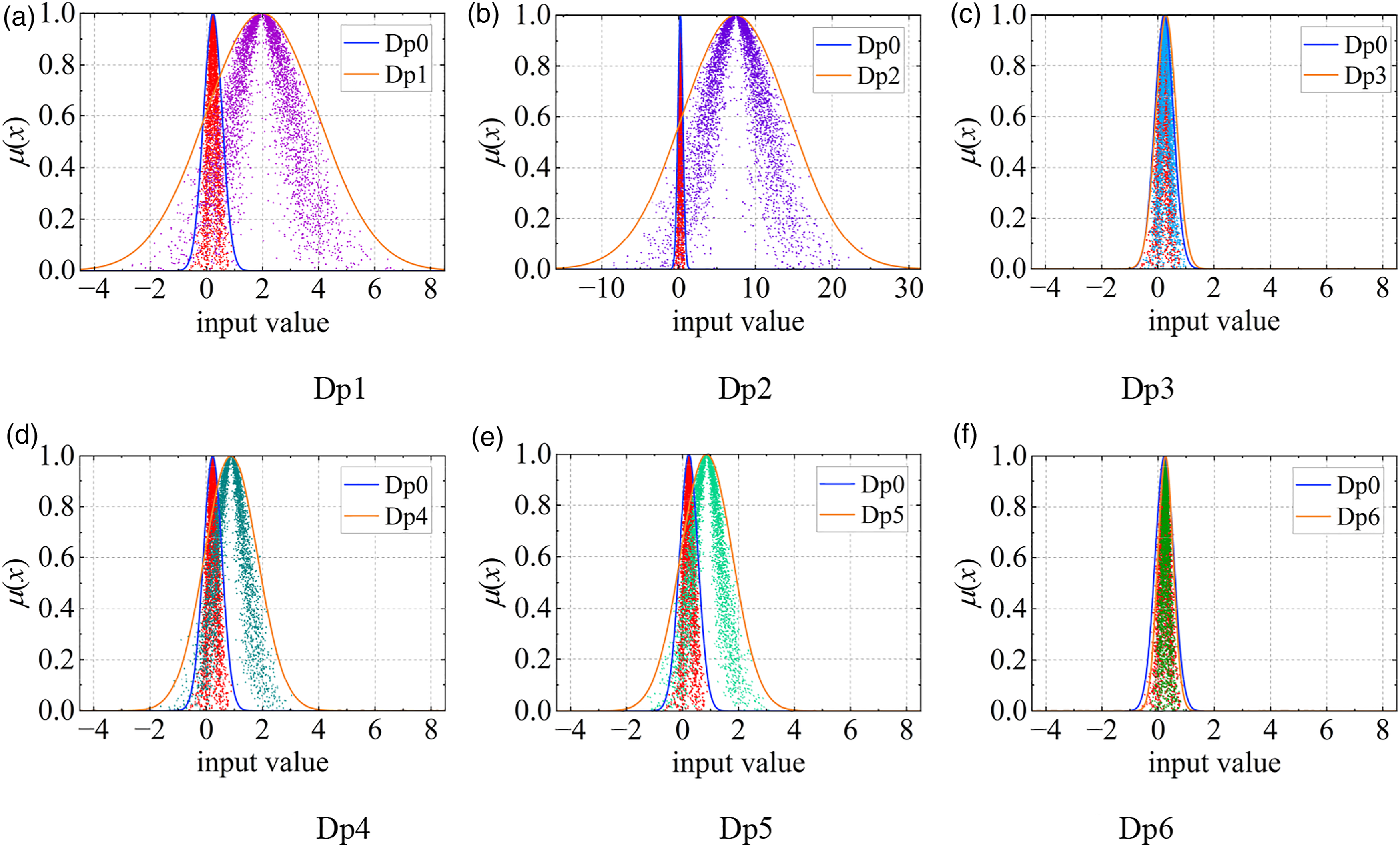

The CM similarity is measured from the MCM, and the S^MCM obtained after normalization of the overlapping regions is shown in Figure 15. The closer the S^MCM is to 1, the more similar the two distributions are, and the less damage is present. With the increase in the degree of damage, the similarity S^MCM gradually decreases. As can be seen from the Figure 15, the noise levels of 5% and 10% have little influence on the damage detection effect, and the damage detection result is good, which is similar to the damage detection result of the data without noise. When the noise level reaches 15%, the loss quantification results of Dp4, Dp5, and Dp6 appear to be affected to some extent. When the noise level is 20%, the detection results of several damage patterns are different from those of the unnoisy data, but it is still consistent with the rule that S^MCM is small when the damage is large.

Figure 15.

S^MCM values obtained after standardization under different noise levels.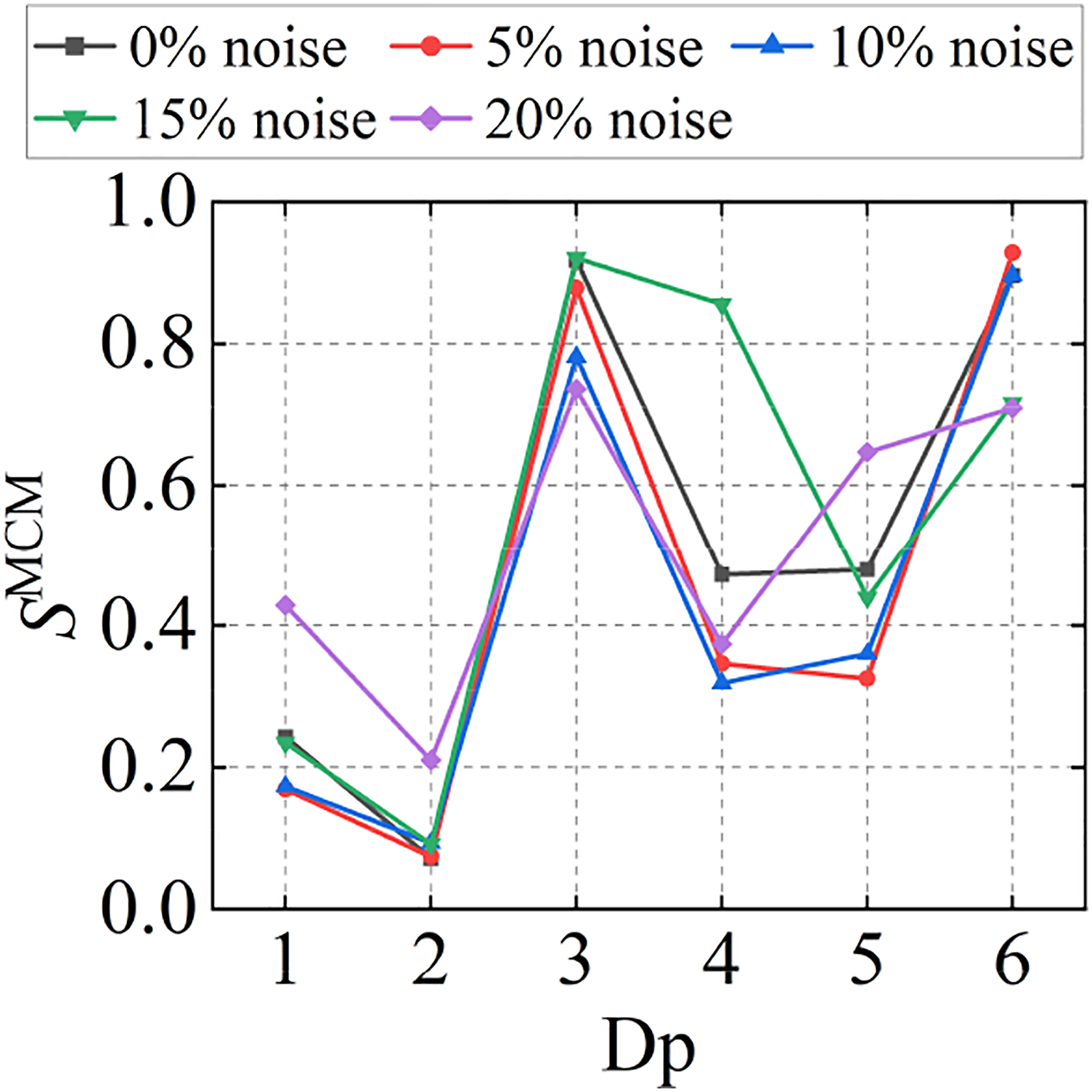

Case study II: A bridge health monitoring benchmark model

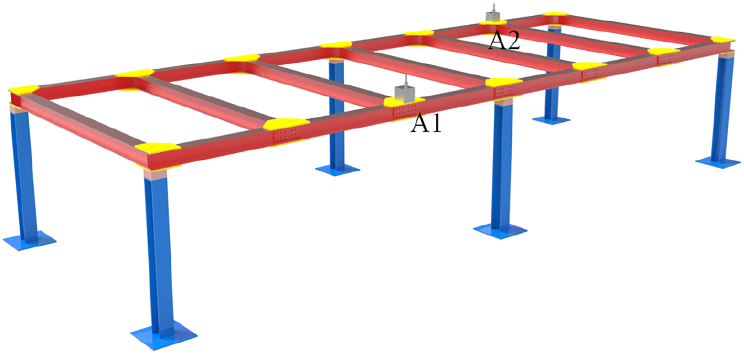
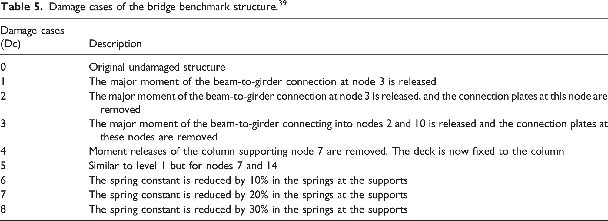
The numerical model of a bridge developed at the University of Central Florida is used to validate the proposed damage detection method. The structure is shown in the Figure 16. The bridge is composed of two girders of length 5.49 m, seven beams 1.83 m long and six W12 × 26 columns of height 1.07 m. All beams have a cross section of S3 × 5.7. Each member of the structure is connected by simple support, hinged support, fixed and semi-fixed, and different types of damage are simulated by controlling boundary conditions, elastic coefficient changes at the support and relaxing the connecting plate. The damage cases are shown in Table 5.

Figure 16.

A schematic of the BHM benchmark structure. ³⁹

Table 5.

Damage cases of the bridge benchmark structure. ³⁹

Damage cases (Dc)	Description
0	Original undamaged structure
1	The major moment of the beam-to-girder connection at node 3 is released
2	The major moment of the beam-to-girder connection at node 3 is released, and the connection plates at this node are removed
3	The major moment of the beam-to-girder connecting into nodes 2 and 10 is released and the connection plates at these nodes are removed
4	Moment releases of the column supporting node 7 are removed. The deck is now fixed to the column
5	Similar to level 1 but for nodes 7 and 14
6	The spring constant is reduced by 10% in the springs at the supports
7	The spring constant is reduced by 20% in the springs at the supports
8	The spring constant is reduced by 30% in the springs at the supports

Caicedo et al. ³⁹ established a numerical simulation model based on Matlab software development in order to facilitate relevant researchers to test their health monitoring techniques. In this study, an instantaneous excitation of 500 N in the vertical direction was applied at the mid-span position of the structure, and the vibration acceleration of the structure was collected by two acceleration sensors with a sampling frequency of 512 Hz and a sampling time of 1 s. The nodes position and sensor placement were shown in Figure 17. The sample size of an accelerometer in each damage case is 512 × 1. In order to enhance the data and simulate the noise in the real environment, random white Gaussian noise of 1%–15% is applied to the original acceleration, and the number of samples of each damage case extended to 500. The data set size of an accelerometer after data expansion is 9 × 500 × 512 × 1. 80% (400) of the health data were randomly selected as the training set, and the remaining 20% (100) of the health data and the data of all the damage cases (8 × 500) were used for testing. Each sample in the data set is normalized to [−1,1]. In the network structure, the latent feature dimension is set to 512, momentum β₁ = 0.9, and other network parameters are the same as in network configurations section.

Figure 17.

Positions of nodes and sensors in the BHM benchmark structure.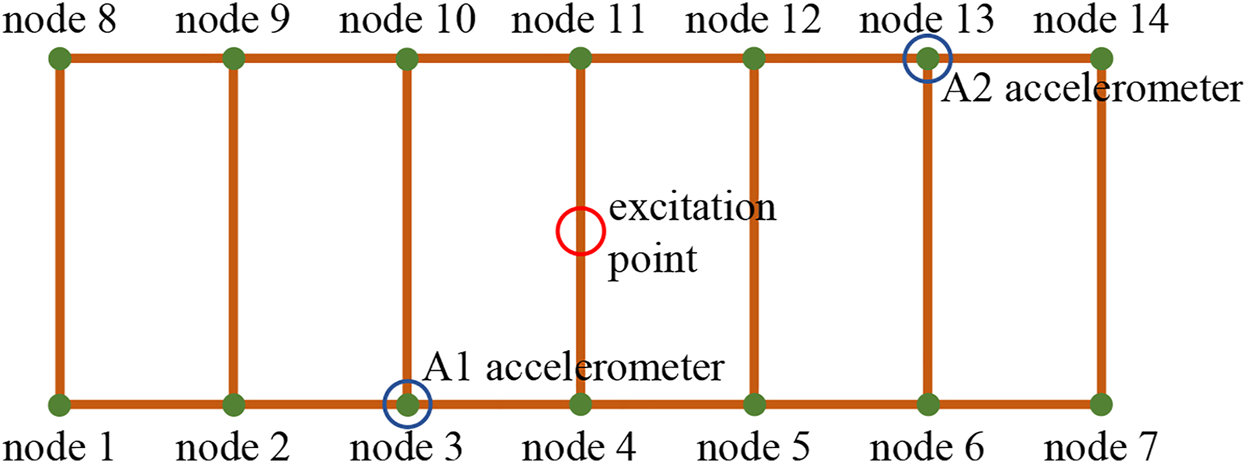

In order to study the influence of sensor position on the damage detection result, the acceleration response of node 3 and node 13 are used for damage detection in this example, respectively. Figure 18 shows the damage detection results of A1 and A2 accelerometers. According to Table 5, Dc1 and Dc2 were both damaged at node 3, and Dc2 was more seriously damaged than Dc1. As can be seen from Figure 18(a), the latent feature differences of Dc1 are around 0.5, while that of Dc2 is around 5. The A1 accelerometer effectively identifies the damage severity of Dc1 and Dc2. As can be seen from Figure 18(b), according to the latent feature differences distribution of the A2 accelerometer, it is impossible to accurately judge which state of Dc1 and Dc2 has more serious damage, and it can only be judged that the structure has damage. The reason may be that the A2 accelerometer is far away from node 3, and the algorithm is not sensitive enough to the damage of the node that is far away. Similarly, Dc5 is the damage at nodes 7 and 14, and the A2 accelerometer with a short distance has better detection results than the A1 accelerometer. Dc6, Dc7, and Dc8 reduce the elastic coefficient of the bearing by 10%, 20%, and 30%, and the damage degree of the structure increases successively. Figure 18 show that both A1 and A2 accelerometers can better quantify the damage at the support, and the damage degree is proportional to the latent feature differences.

Figure 18.

Distributions of latent feature differences in the test set. (a) A1 accelerometer (b) A2 accelerometer.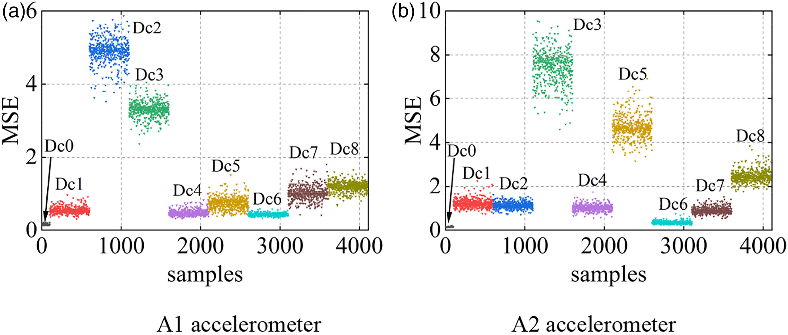

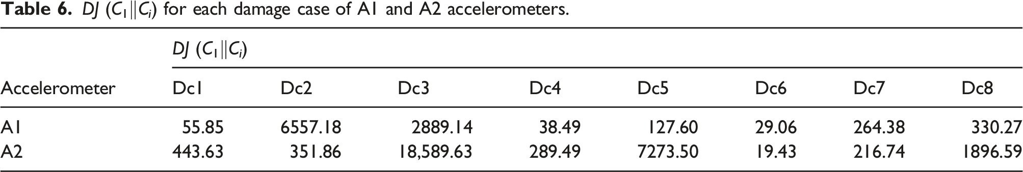
The normalized damage index S^MCM obtained based on MCM is shown in Figure 19. In some damage cases, the damage degree is larger and the S^MCM value is [0,1], so it is impossible to accurately judge that the damage in that state is more serious. Therefore, KLD based on MCM is used to quantify structural damage, as shown in Table 6. In the case of large damage, when S^MCM is 0, DJ (C₁‖C _i ) can be added for judgment, and DJ (C₁‖C _i ) has better damage quantification effect than S^MCM. Overall, the network trained according to the data collected by sensors in different positions can effectively judge whether the structure is damaged, but it has certain influence on the judgment of the damage degree between the damaged position and various cases, and some misjudgments may occur. The sensors near the damage location are more sensitive to the damage degree, and the judgment accuracy is higher. Therefore, in order to accurately locate the damage position of the structure, multiple sensors in different positions should be used for comprehensive evaluation.

Figure 19.

Distributions of latent feature differences in the test set.

Table 6.

DJ (C₁‖C _i ) for each damage case of A1 and A2 accelerometers.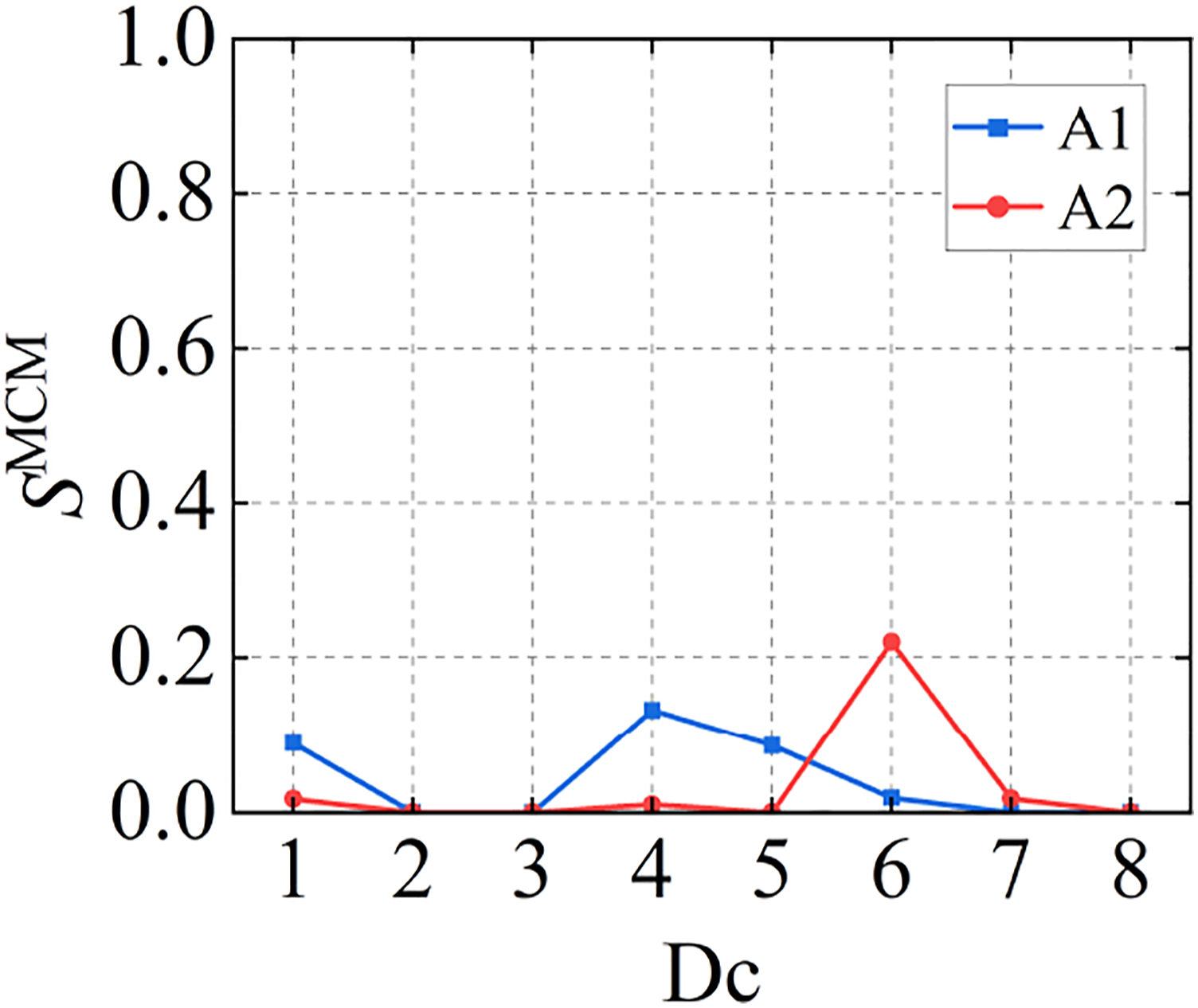

Accelerometer	DJ (C1‖C i )
	Dc1	Dc2	Dc3	Dc4	Dc5	Dc6	Dc7	Dc8
A1	55.85	6557.18	2889.14	38.49	127.60	29.06	264.38	330.27
A2	443.63	351.86	18,589.63	289.49	7273.50	19.43	216.74	1896.59

Conclusion

An unsupervised damage detection method based on IGAN and CM is proposed. The damage detection capability of the proposed method is verified by the Phase I IASC-ASCE benchmark structure and a bridge health monitoring benchmark model. Based on the analysis, conclusions can be drawn as follows.

(1) The proposed damage detection method has noise immunity to an extent, and it still has good damage detection results at 15% noise level. When the noise level reaches 20%, the damage detection accuracy decreases slightly. In the actual engineering structure, the method can meet the engineering application due to the noise level is mostly below 15%.

(2) The structural damage indicator S^MCM can distinguish different degrees of structural damage under conventional conditions. When the structural damage is too large, S^MCM is 0, and accurate results cannot be obtained based on S^MCM alone. It can be judged by supplementing another structural damage index DJ, which can obtain better damage quantification effect.

(3) The influence of structural damage at different locations on different sensors is different, so it is essential to use as many sensors as possible for comprehensive structural damage evaluation. The performance of the algorithm will be tested in a more realistic environment in subsequent work and accurate damage localization of the bridge structure is going to be considered as well.

(4) The proposed method only requires the normal operating state data in the training phase, and utilizes the difference of latent feature difference range between the unknown state samples and the healthy samples for damage detection in the test. It provides a practical damage detection method for structures without requiring any information from their damage states. However, the proposed damage index reflects the deviation between the current structural state and the healthy state, and the relationship with the actual physical quantity has not been established. In practice, the damage warning can be realized by properly setting the damage threshold.