Sage Journals: Discover world-class research

Abstract

A defective structure has been evaluated and identified in beam models’ deflection measurement signals in much research. However, many results have not been optimally exploited and evaluated to find new parameters for data excavation. This manuscript proposes a cumulative welding model and a cumulative circle of deflection signals for a defective beam under the impact of a moving force. Based on this evaluation model, the manuscript recognizes that the speed of the moving force will determine the regression speed of the received datasets, which is considered the basis for showing the working ability of a beam structure with defects. Moreover, the structure’s cumulative regression circle also shows its resilience in that structure after the impact of the load. The development of defects in the structure will depend on both the structure’s level and resilience after each bearing-load cycle. Our research has shown us that the method of evaluation and use of both the cumulative model and cumulative circle from the deflection’s measured value have yielded more results compared to the previous method. This research can evaluate many defects in different situations while simultaneously evaluating many types of structures.

Keywords

Cumulative function cumulative circle structure defect deflection beam model

Introduction

The appearance of defects introduces potential risks during a structure’s operation. Many dangers can be imposed on people and property because of such defects arising suddenly. Many methods have been proposed for the process of assessing the emersion as well as the defect growth that exists in a structure. Therefore, evaluating the occurrence of defects plays an extremely important role in many different fields. In terms of applications, this research can be applied to many different types of structures today: a structural model in the shape of a bar, a beam, a plate, or a combination of two or more of these mentioned components. Structures that have been simulated under the bearing-force conditions of the beam model the most popular rate because of optimization in calculations and simple experiments. In such cases, the management units are always interested in the process of evaluating and forecasting the structure’s quality to have reasonable exploitation methods and to guarantee regular maintenance and suitable repairs. Furthermore, warnings in the case of a breakdown or problems in a structure may occur in either the present or future. Many suitable methods have been applied to evaluate the prediction of damage in recent studies on structures.^1,2 However, the common point of these methods often uses the difference between the measured data in different measurement intervals. In this study, the measured data at time t will be used as a standard to make forecasts and warnings at time t + Δt, in which Δt is the time interval calculated from the initial measurement point t.³

Research on the influence of defects on beam structure has been carried out many times,^4,5 with many new parameters being proposed for evaluating and identifying the existence of defects in beams. Authors have approached the beam model with the force-bearing condition of a single girder with a continuous structure and two-headed support at the connectors.⁶ The model’s force-bearing state will be changed depending on the actual level and requirements and the actual structure’s force-bearing state. Defects can appear in the actual structural model and exist in many forms, such as small cracks in the structure, aging of the structure over elapsed time, and physical and chemical agents from either the external environment or direct external stimulus. Therefore, many modeling methods have attempted to describe defects in real structures in terms of modeling beam structures. Of many different assumptions, the most important is that the defects in a model will cause the beam’s force-bearing capacity to be directly affected. The defects will then change either the dimensions or the geometry of the structure,^7–9 or the structure will change internally through changes in the material’s mechanical properties.^10–13 Researchers often demonstrate defects using the crack model implemented in the laboratory,^1,2,14,15 with shapes of geometrical cuts, such as cutting, cross-cutting, longitudinal cutting, and depth cutting, or changes of the cutting geometry,^16,17 such as circular cutting, oval cutting, and oblique cutting. Apart from this, many studies have also looked at the deterioration of the material mechanical properties, such as the elastic modulus,¹⁸ the modulus of torsion resistance, or the aggregate of the above factors. All the changes created in the beam model are attributed to a single condition to reduce the structure’s stiffness.^19,20

When the load moves on the beam model, whether the beam has defects or not, three significant mechanical changes always appear: beam vibration under load impact, structure deformation, and model deflection.^1,2,21–24 The signal obtained from the deflection value is used frequently and ensures much higher efficiency in the process of determining the presence of defects in the structure.^25–27 The results show that the evaluation of defects existing in a structure by the deflection value always yields positive results. Moreover, along with the development of modern science through models of both big data and machine learning, many researchers want to increase signal sensitivity so that it can be investigated through optimal algorithms, such as certain statistical methods^28,29 combined with optimal algorithms,^30–32 combined with algorithms of artificial neural networks,^33–35 or investigated in combination with wavelet analysis^36,37 or neural-fuzz techniques.³⁸ Moreover, many researchers have converted signals into intermediate signals for greater efficiency compared to the original signal. We can mention the projects that have transmitted signals into load vectors,³⁹ the Ritz vector,^40,41 elastic deformation potential energy,⁴² or wavelet signals.³⁶ The resulting advantageous trend is that the problems posed can be tackled with a much more efficient use of data resources. However, these studies have the disadvantage of processing only the data algorithms without looking for and solving the drawbacks in the given system. Therefore, the practical problems have not been solved thoroughly and effectively, despite the many accompanying algorithms. Considering the drawbacks of previous studies, this manuscript uses a model that searches for the occurrence of defects in the beam structure with the condition in which the load moves through the method of the cumulative function and the cumulative circle of the deflection values. This model can evaluate many structures’ different behavior states if they are actually applied through experimental models with many different boundary conditions.^43,44 Through the processing of input parameters, the manuscript will offer parameters that can evaluate the changed degree of structural defects. At the same time, this manuscript will improve the model⁴⁴ for evaluating defect growth in structures’ various boundary conditions.

Theoretical basis

Displacement model of the load-bearing beam structure

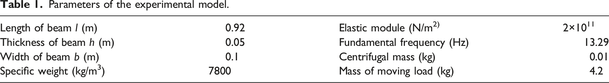
This manuscript has modeled a thin beam structure with length l, where the model’s boundary condition is two-headed support, the bearing state is mainly shear force, and the load impacting on the model is dynamic load, which can move along the beam length, as shown in Figure 1.^3–5 This movable load primarily exerts force in the direction perpendicular to the beam, which mainly causes the beam to be in a bending state. From there, the manuscript will survey the load’s influence on the beam response.

Figure 1.

Simplified beam model with a moving load forming the deflection.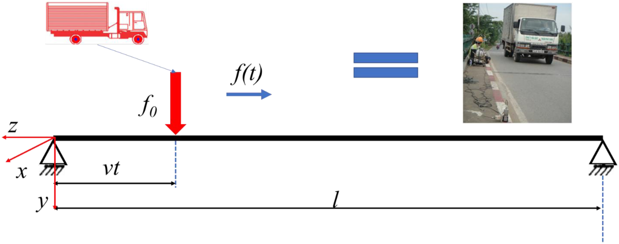

According to Fryba L,⁴⁵ the vibration equation of the flexural beam with the system of impact force, as shown in Figure 1, is demonstrated in equation (1)

E J \frac{\partial w^{4} (x, t)}{\partial x^{4}} + ρ \frac{\partial w^{2} (x, t)}{\partial t^{2}} + 2 ρ ω_{d} \frac{\partial w (x, t)}{\partial t} = δ (x - υ t) f (t)

(1)

with boundaries and initial conditions

\begin{array}{l} w (0, t) = 0; w (l, t) = 0, \\ {\frac{\partial^{2} w (x, t)}{\partial x^{2}} |}_{x = 0} = 0; {\frac{\partial^{2} w (x, t)}{\partial x^{2}} |}_{x = l} = 0 \end{array}

(2a)

w (x, 0) = 0; {\frac{\partial w (x, t)}{\partial t} |}_{t = 0} = 0;

(2b)

in which x is the coordinates of the concentrated force calculated from the coordinates axis from the left end of the beam, t is the moving time with the time origin once the load begins impacting on the beam, w (x, t) is the beam displacement at position x and time t, ρ is the specific weight of the beam per unit length, ω_d is the damping frequency, f(t) is the force amplitude, l is the beam length, υ is the load velocity, and $δ (.)$ is the impulse function. The manuscript has used the Galerkin method^46–48 to solve equation (1), which is one of the most suitable approximations for solving various problems of structural dynamics. The root of equation (1) is still chosen as the dissociation of variables, in which the function ϕ_j(x) is linearly independent, satisfying the boundary conditions of the structural model in equations (2a) and (2b), and the function q_j(t) is a time-varying function that is determined from the integral of the ordinary partial derivative equation.

\int_{0}^{l} {L [\sum_{j = 1}^{n} q_{j} (t) ϕ_{j} (x)] - f (x, t)} ϕ_{j} (x) d x = 0

(3)

With the boundary condition in equation (2a), we choose the function ϕ(x) = sin(jπx/l) and then integrate the terms with the bounds from 0 to l; thus, we have the transformation of the sine Fourier integral^49–51 as follows

w (x, t) = \frac{2}{l} \sum_{j = 1}^{\infty} W (j, t) \sin \frac{j π x}{l}

(4a)

W (j, t) = \int_{0}^{l} w (x, t) \sin \frac{j π x}{l} d x, j = 1,2,3, . . .

(4b)

Substituting equation (4a) into equation (3), after integration, we receive equation (5)

\frac{j^{4} π^{4}}{l^{4}} E J W (j, t) + ρ \ddot{W} (j, t) + 2 ρ ω_{b} \dot{W} (j, t) = \int_{0}^{l} \partial (x - υ t) f (t) \sin \frac{j π x}{l} d x

(5)

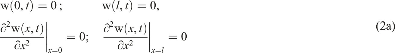
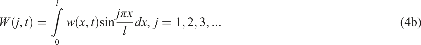
We consider the harmonic load f(t) = Q₀sin (Ωt + θ) in which Q is the load amplitude, Ω is the constrained frequency, and θ is the initial phase, as shown in Figure 2. Then, equation (6) becomes the following

p^{2} W^{*} (j, p) + 2 ω_{b} p W^{*} (j, p) + ω_{j}^{2} W^{*} (j, p) = p \frac{Q}{2 ρ} \int_{0}^{\infty} [\cos ((Ω - j ω_{υ}) + θ) - \cos ((Ω + j ω_{υ}) + θ)] e^{- p t} d t

(6)

Figure 2.

Model of harmonic load moving on beams with a previously given impact.

Beginning with this research, our manuscript proposes a complex level of harmonic force by adding more of the initial phase θ. Because we find it difficult to determine the initial phase of the harmonic phenomenon when conducting the actual experiment, the manuscript has been extended to case θ, which is a random variation with a value between 0 to 2π.

Set: Ω₁ = Ω + jω_υ, and Ω₂ = Ω − jω_υ

We have

W^{*} (j, p) = \frac{f (t)}{2 ρ} [p^{2} \cos θ (\frac{1}{p^{2} + r_{2}^{2}} - \frac{1}{p^{2} + r_{1}^{2}}) - p \sin θ (\frac{Ω_{2}}{p^{2} + r_{2}^{2}} - \frac{Ω_{1}}{p^{2} + r_{1}^{2}})] \frac{1}{{(p + ω_{b})}^{2} + ω_{d j}^{2}}

(7)

Transforming the inverse Laplace–Carson,^52,53 we have the original function W(j, t). Substituting it into equation (4a), we obtain the following

w (x, t) = \frac{f (t)}{l ρ} \sum_{j = 1}^{\infty} [\cos θ (A (Ω_{2}) - A (Ω_{1})) - \sin θ (Ω_{2} B (Ω_{2}) - Ω_{1} B (Ω_{1}))] \sin \frac{j π x}{l}

(8)

with

A (Ω) = \frac{1}{{(ω_{j}^{2} - Ω^{2})}^{2} + 4 ω_{b}^{2} Ω^{2}} [(ω_{j}^{2} - Ω^{2}) (c o s Ω t - e^{- ω_{b} t} c o s ω_{j} t) + 2 ω_{b} Ω s i n Ω t - \frac{ω_{b}}{ω_{d j}} (ω_{j}^{2} + Ω^{2}) e^{- ω_{b} t} \sin ω_{d j} t]

B (Ω) = \frac{1}{{(ω_{j}^{2} - Ω^{2})}^{2} + 4 ω_{b}^{2} Ω^{2}} [\frac{ω_{j}^{2} - Ω^{2}}{Ω} \sin Ω t - \frac{ω_{d j}^{2} - ω_{b}^{2} - Ω^{2}}{ω_{d j}} e^{- ω_{b} t} \sin ω_{d j} t - 2 ω_{b} (\cos Ω r t - e^{- ω_{b} t} \cos ω_{d j} t)]

Building the signal amplitude accumulation model

Data distribution is an important factor in evaluating the trustworthiness of a dataset. Through its distribution, we can evaluate the data changes in different statuses. The data can be conducted by the active cause created by the impact force or by noise during the measurement. Studies with the main purpose of evaluating the nature of the dataset often use the probability distribution function, which is shown on the curve of the Gaussian probability distribution functions, as shown in Figure 4(c), and illustrated in equations (9a) and (9b).

P (X \geq x) = \frac{1}{\sqrt{2 π σ}} \int_{x}^{\infty} \exp {- \frac{1}{2} {(\frac{x - \bar{x}}{σ})}^{2}} d x

(9a)

P (X < x) = 1 - \frac{1}{\sqrt{2 π σ}} \int_{- \infty}^{x} \exp {- \frac{1}{2} {(\frac{x - \bar{x}}{σ})}^{2}} d x

(9b)

If $\frac{x - \bar{x}}{σ} = z$ , is normalized, then z is called a standardized variable. Provided that the distribution of z values is in the range N (0, 1), equations (9a) and (9b) is changed by equations (10a) and (10b)

P (X \geq x) = \frac{1}{\sqrt{2 π σ}} \int_{x}^{\infty} \exp {- \frac{1}{2} z^{2}} d x = Φ (z)

(10a)

P (X < x) = 1 - \frac{1}{\sqrt{2 π σ}} \int_{- \infty}^{x} \exp {- \frac{1}{2} z^{2}} d x = 1 - Φ (z)

(10b)

Here, the function Φ(z) is called the cumulative distribution function (CDF) for N (0, 1). The cumulative distribution function has been surveyed less compared to the Gaussian distribution function, but the illustration of the distribution value is clearer, as shown in Figure 4(a). Apart from the cumulative function, this manuscript also proposes a cumulative circle model of the surveyed values, as shown in Figure 4(b) (C-CDF). Figure 3 depicts a set of actual data measured in three directions, Ox, Oy, Oz, to evaluate the difference of this dataset corresponding to the three directions illustrated by two parameters: PDF and CDF. The graph demonstrating the PDF value is shown in Figure 4(c), while the CDF is shown in Figure 4(a).

Figure 3.

Set of actual acceleration signals in three directions: Ox, Oy, Oz. (a) Acceleration signal in the direction of Ox. (b) Acceleration signal in the direction of Oy. (c) Acceleration signal in the direction of Oz.

Figure 4.

CDF, C-CDF, PDF distribution rules of the signal set, as shown in Figure 3. (a) CDF distribution rules; (b) C-CDF distribution rules; (c) PDF distribution rules.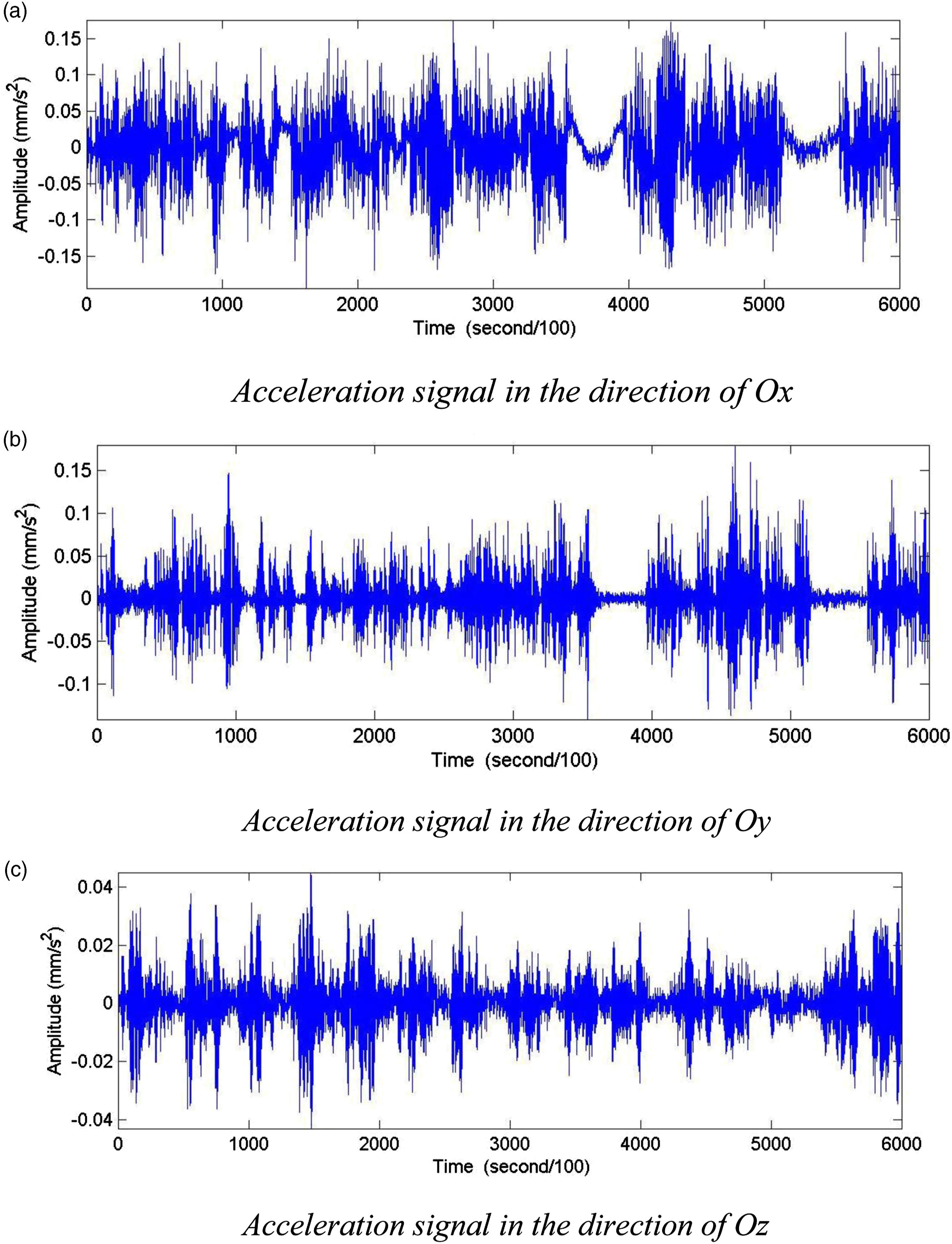

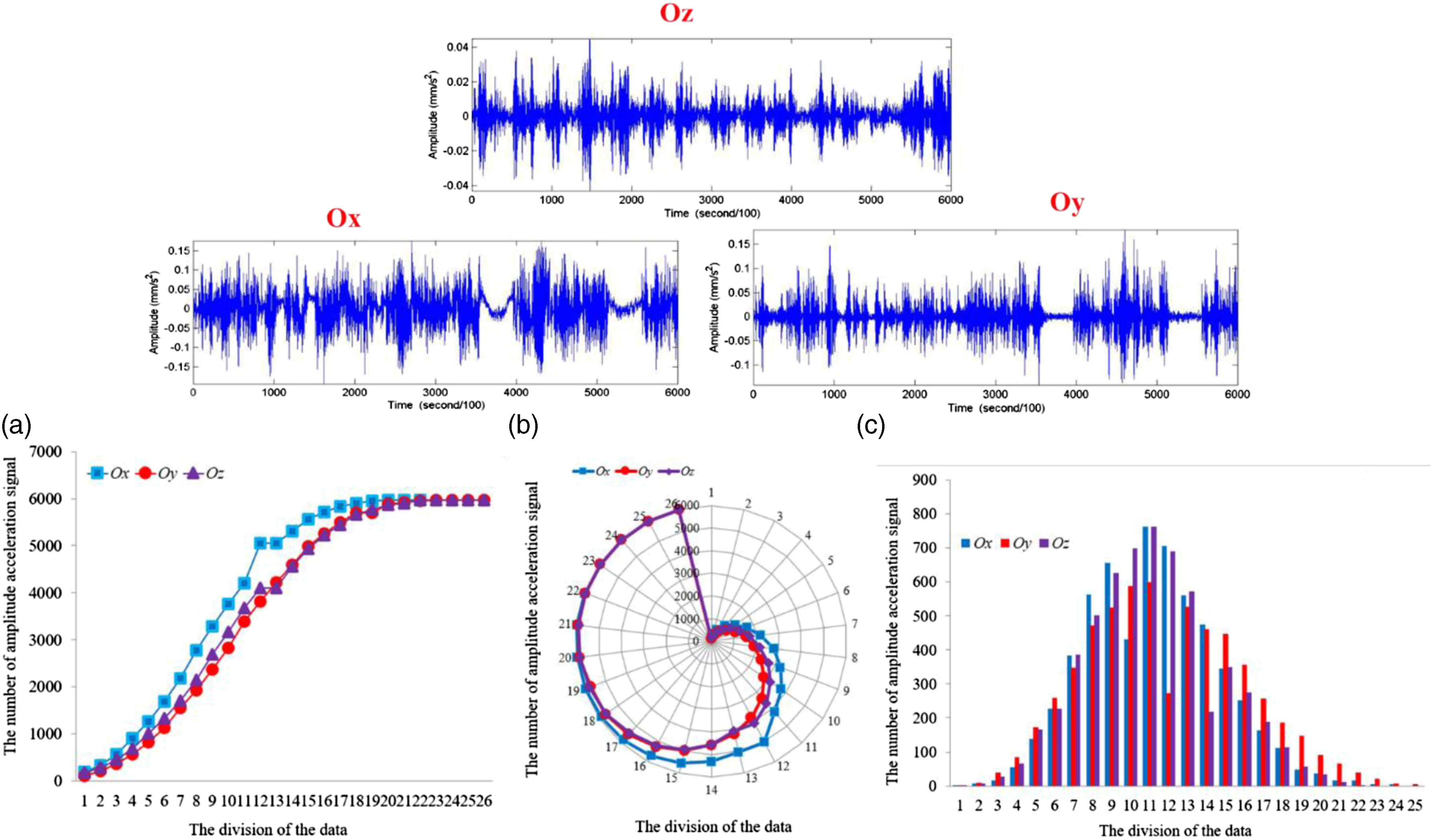
As can be seen in Figure 3, the difference between the graphs obtained from this dataset is very small, so the research will look for their differences through the distribution rule of CDF and C-CDF. This manuscript proposes to use the characteristics of both CDF (Figure 4(a)) and C-CDF (Figure 4(b)) for this research when evaluating the change in signal patterns over time. Thanks to these two characteristics, we have been able to form a new evaluation method through which we can survey in detail the change of datasets within and between datasets over different durations. As shown in Figure 4(c), three signal samples measured at a point in three different directions were surveyed. The result when using the PDF model does not clearly demonstrate the degree of change and difference between these datasets. In contrast to PDF, the distribution of CDFs has shown clearer variation between them compared to the distribution of PDF values. In addition, C-CDF also displayed the speed and convergence of the surveyed data. This can be considered this research’s outstanding feature compared with the process of identifying and evaluating the changes of signals used in previous research.

This manuscript proposes to use the signal’s distribution model to represent the difference of the signal over each stage, as shown in Figure 4(a) and (b). As shown in these figures, the difference between the stages of beginning to those of growth is very large in all three datasets, although the datasets converge almost simultaneously and equally in the last data intervals. Based on the characteristics of the above data, the data will destabilize in each specified interval; the more different datasets there are, the more unstable intervals there will be, and vice versa. However, we will be able to evaluate the convergence level in the data’s convergence phase as well as the quality in which the dataset is illustrated. In this way, this manuscript opens up a new evaluation method for exploiting and processing the data via.

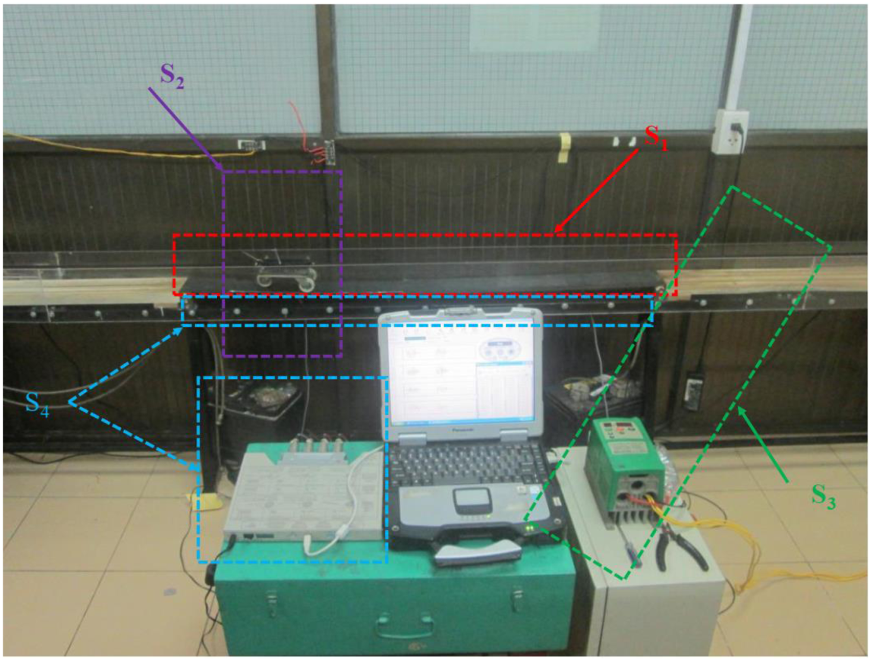
Experimental model

The experimental model manufactured includes the main equipment: beam frame (S₁), moving load (S₂), vehicle transmission system (S₃), including inverter and motor, and measuring sensor (S₄).

Beam model (S₁): the structure includes a steel beam with the dimensions shown in Table 1. The beam is leaned on two supportive abutments, with a rubber pad used for the attachment of the beam to reduce the beam’s impact. In addition, the deflection measurement sensor is placed on the beam in different positions to match the theoretical model, as shown in Figure 5.

Table 1.

Parameters of the experimental model.

Length of beam l (m)	0.92	Elastic module (N/m²⁾	2×10¹¹
Thickness of beam h (m)	0.05	Fundamental frequency (Hz)	13.29
Width of beam b (m)	0.1	Centrifugal mass (kg)	0.01
Specific weight (kg/m³)	7800	Mass of moving load (kg)	4.2

Figure 5.

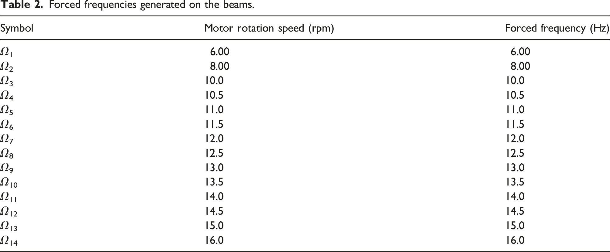
Conducting the vibration measurements on the beams.

Mobile loading model (S₂): a structure produced from a metal block is connected to the transmission system with an inextensible wire for the load to move on the beam. An additional eccentric block is installed on the shaft of the motor to create harmonic force with any frequency by f(t) = Q₀sin(ῼt). The model can change the motor’s rotational speed through the inverter shown in Table 2. The manuscript can create a force that can vary both the magnitude of the impacted force and the frequency of the different excitation forces, as required by the theoretical model and shown in Figure 8.

Table 2.

Forced frequencies generated on the beams.

Symbol	Motor rotation speed (rpm)	Forced frequency (Hz)
Ω ₁	6.00	6.00
Ω ₂	8.00	8.00
Ω ₃	10.0	10.0
Ω ₄	10.5	10.5
Ω ₅	11.0	11.0
Ω ₆	11.5	11.5
Ω ₇	12.0	12.0
Ω ₈	12.5	12.5
Ω ₉	13.0	13.0
Ω ₁₀	13.5	13.5
Ω ₁₁	14.0	14.0
Ω ₁₂	14.5	14.5
Ω ₁₃	15.0	15.0
Ω ₁₄	16.0	16.0

The transmission system for the load (S₃) consists of a three-phase motor, transmission belt, and inverter control. The system has the transmission effect to help the load move on the beam at different speeds, as shown in Table 3. In this research, the manuscript will simulate the difference of loads and velocities on the beam with the speed of the load v, in which the experimental model is calculated based on the homothetic relationship between the rate of the moving frequency and fundamental frequency.

Table 3.

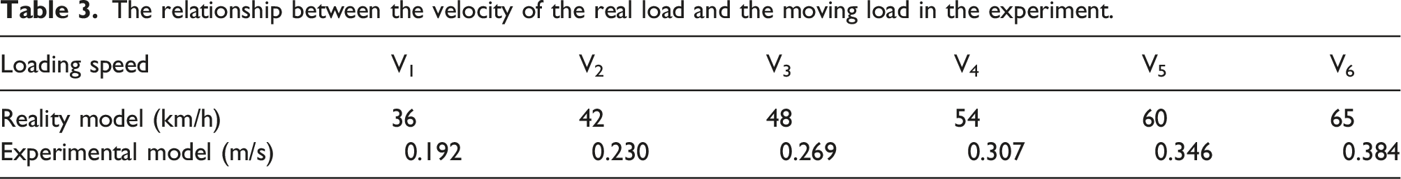
The relationship between the velocity of the real load and the moving load in the experiment.

Loading speed	V₁	V₂	V₃	V₄	V₅	V₆
Reality model (km/h)	36	42	48	54	60	65
Experimental model (m/s)	0.192	0.230	0.269	0.307	0.346	0.384

The measuring system (S₄) includes four sensors (D₁, D₂, D₃, D₄) installed evenly and distributed along the experimental beam.

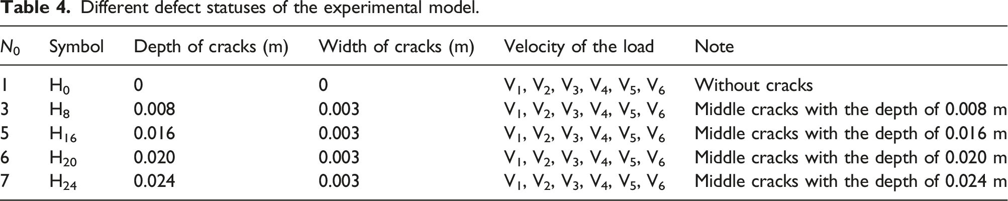
Beams measured in many different defect statuses are shown in Table 4, and the excitation forces are shown in Figure 5. The defects are described by cuts with different cross-sectional profiles, such as small cuts according to the beam depth and cuts on both sides of the beams. All cracks were created by the cutting method with complete precision to facilitate the evaluation process and determine the relationship between the ability to reduce hardness and the growth of the defect. Figure 6 shows how the measurement procedure is carried out.

Table 4.

Different defect statuses of the experimental model.

N ₀	Symbol	Depth of cracks (m)	Width of cracks (m)	Velocity of the load	Note
1	H₀	0	0	V₁, V₂, V₃, V₄, V₅, V₆	Without cracks
3	H₈	0.008	0.003	V₁, V₂, V₃, V₄, V₅, V₆	Middle cracks with the depth of 0.008 m
5	H₁₆	0.016	0.003	V₁, V₂, V₃, V₄, V₅, V₆	Middle cracks with the depth of 0.016 m
6	H₂₀	0.020	0.003	V₁, V₂, V₃, V₄, V₅, V₆	Middle cracks with the depth of 0.020 m
7	H₂₄	0.024	0.003	V₁, V₂, V₃, V₄, V₅, V₆	Middle cracks with the depth of 0.024 m

Figure 6.

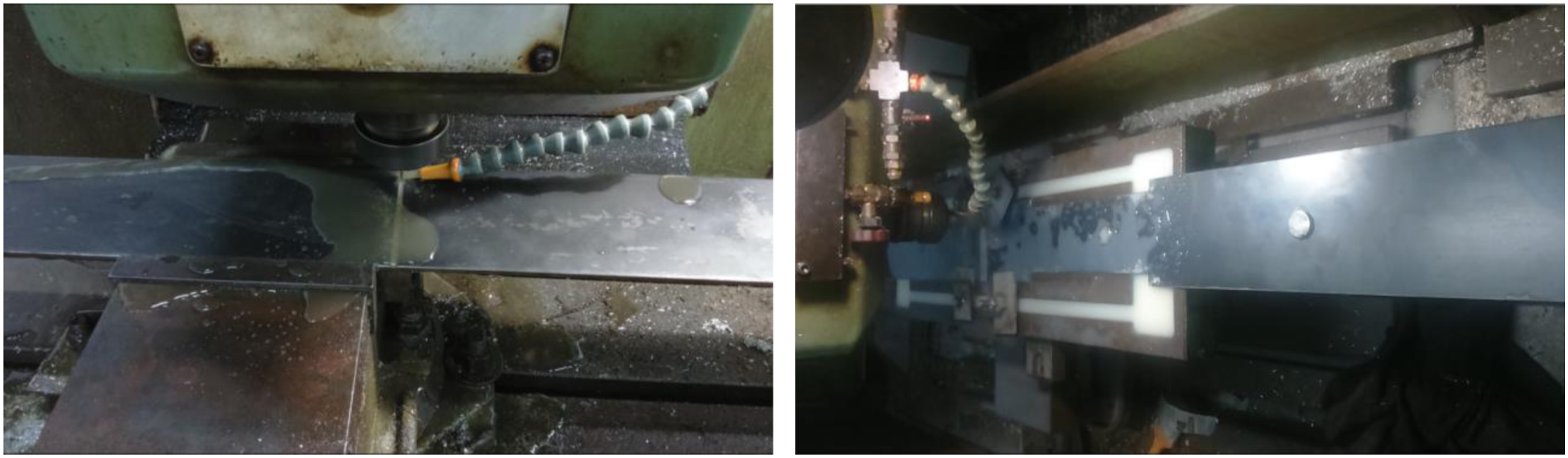
Defects generated on the beams.

Results and comments

Evaluating the deflection of the experimental model under the influence of a moving load as compared against the theory

According to the theory discussed in Section theoretical basis, the maximum deflection of the moving concentrated force is equal to the static deflection at the middle of the beam, according to equations (9a) and (9b). When x = l/2 (i.e., is at the middle point in the beam), the maximum deflection of the static deflection will be equal to the moving concentrated force. After conducting experiments with moving loads on the beams, as in Refs.^54,55 we will get the beam’s deflection signals corresponding to different excitation conditions, as shown in Figure 7.

Figure 7.

The signal received from the translocation sensor corresponding to the levels of velocity V₁.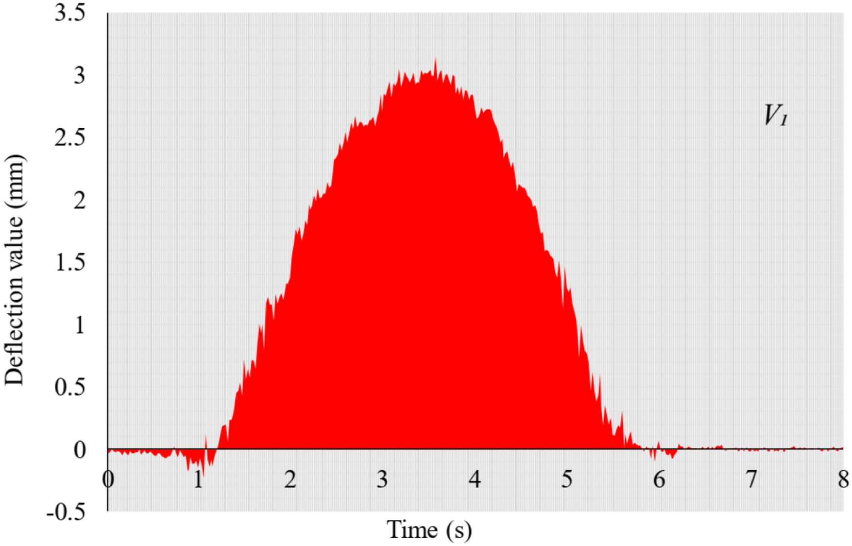

The beam’s deflection graph is shown in Figure 7, with the moving speed of load V₁ performing the experiments at many different speeds from V₁ to V₆. The results obtained are shown in Figure 8 and Table 5. The results demonstrate the following points.

Figure 8.

Model deflection in various velocity statuses.

Table 5.

Deflection from experiment and theory under the influence of a moving load.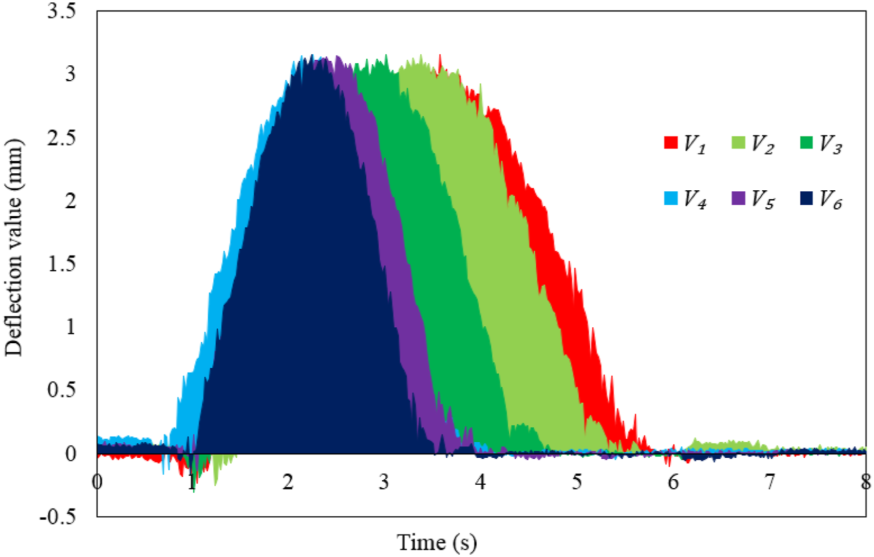

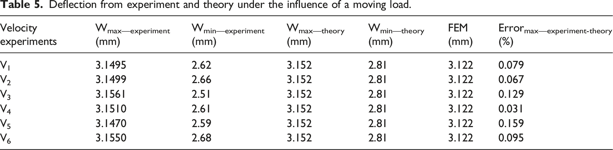
Velocity experiments	W_{max—experiment} (mm)	W_{min—experiment} (mm)	W_max—theory (mm)	W_min—theory (mm)	FEM (mm)	Error_{max—experiment-theory} (%)
V₁	3.1495	2.62	3.152	2.81	3.122	0.079
V₂	3.1499	2.66	3.152	2.81	3.122	0.067
V₃	3.1561	2.51	3.152	2.81	3.122	0.129
V₄	3.1510	2.61	3.152	2.81	3.122	0.031
V₅	3.1470	2.59	3.152	2.81	3.122	0.159
V₆	3.1550	2.68	3.152	2.81	3.122	0.095

The static deflection value obtained from the experiment is smaller than the static deflection value obtained from the theory. This can be explained by the fact that the theoretical model has modeled the forces impacting the wheels and causing a concentrated force P to be generated. As a matter of fact, however, the force pattern on the wheel is evenly distributed at four other points. Because the characteristics of the experimental model are much smaller than those of the actual model, the load force will have a smaller impact on the model. Thereby, this manuscript considers that the forces distributed at the model’s wheels when the vehicle is moving on the beam can be attributed to a single concentrated force, as in the theory, without affecting the results of the model’s analysis and allowing a simplification of the abacus model.

As shown in Figure 8, when many models’ different velocity statuses on the beam are changed, the experiment’s maximum velocity value will not change. The results are shown in Table 5. This shows that the velocity value does not affect the deflection of the actual structure. In other words, according to this evaluation method, the structure of the existing project will not be affected by the influence of different speeds.

Evaluating the influence of the stimulus conditions between the theory and experiment

Influence of the speed and frequency of the constraining force on deflection

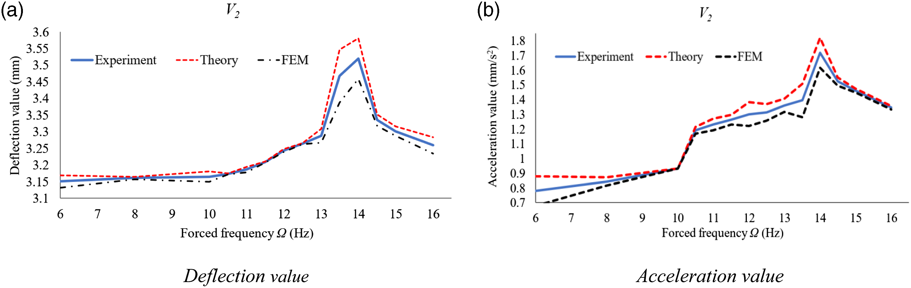
The main purpose of this manuscript is to evaluate the impacts of the harmonic force when the load moves on the beam in terms of the speed and frequency of the different excitation forces. This manuscript has compared the results obtained from the experimental procedure, the results from the theory, and the results calculated by the finite element method (FEM) to evaluate the results. The results are shown in Figure 9(a) and (b) and Figure 10(a) and 10(b).

Figure 9.

Values of deflection and acceleration obtained by different constraining forces Ω with velocity V₁ = 0.192 m/s. (a) Deflection value. (b) Acceleration value.

Figure 10.

Values of deflection and acceleration obtained by different constraining forces Ω with velocity V₃ = 0.23 m/s. (a) Deflection value. (b) Acceleration value.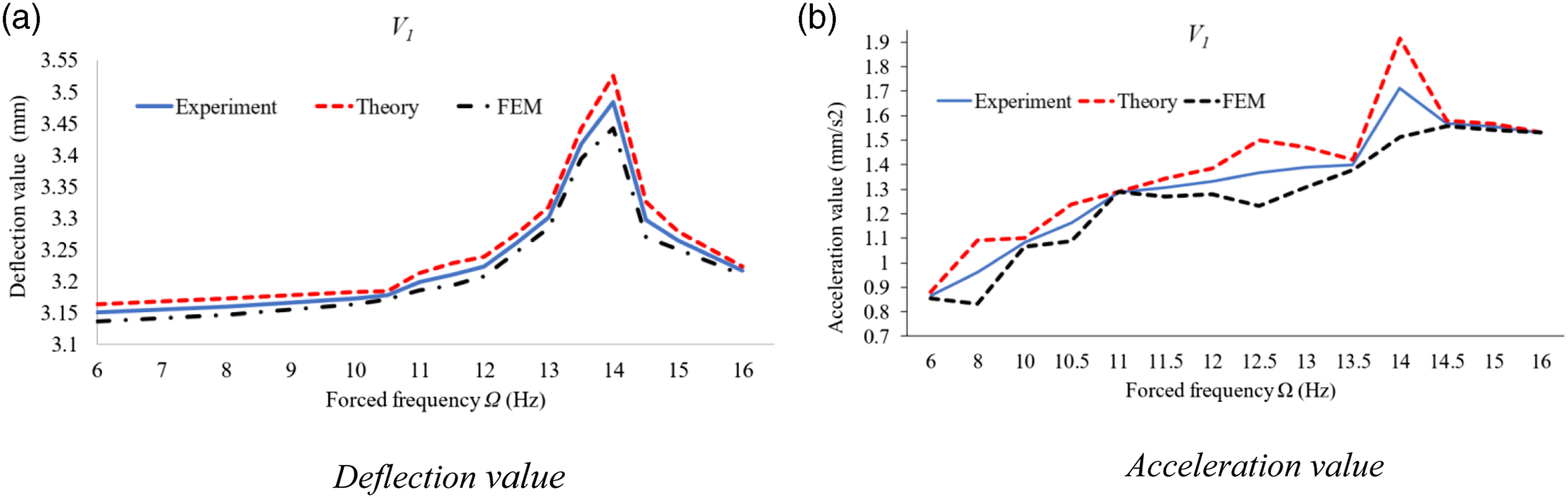

The deflection’s amplitude value and the acceleration’s amplitude value obtained from this manuscript always reach the highest value at the frequency region Ω = 14 Hz, which is also the value at the beam’s dedicated frequency. When the value of the dedicated frequency coincides with the value of the dedicated frequency in the system, the resonance status is reached, and then this state can cause damage or the destruction of the structure. In fact, we need to pay attention to this phenomenon to avoid damage to the structure; at the same time, we should consider a safety measure for the structure. The detailed results are shown in Table 6.

Table 6.

Deflection values corresponding to different excitation frequencies.

Symbol	V₁ = 0.192 m/s			V₂ = 0.23 m/s			V₃ = 0.269 m/s
Symbol	Exp	Theory	FEM	Exp	Theory	FEM	Exp	Theory	FEM
Ω₁ = 6.00 Hz	3.15	3.17	3.153	3.15	3.16	3.165	3.15	3.15	3.158
Ω₂ = 8.00 Hz	3.16	3.16	3.168	3.16	3.16	3.164	3.16	3.16	3.165
Ω₃ = 10.0 Hz	3.18	3.18	3.168	3.17	3.18	3.179	3.16	3.18	3.182
Ω₄ = 10.5 Hz	3.19	3.19	3.189	3.18	3.19	3.189	3.17	3.19	3.184
Ω₅ = 11.0 Hz	3.20	3.19	3.195	3.19	3.19	3.192	3.19	3.19	3.195
Ω₆ = 11.5 Hz	3.21	3.21	3.212	3.21	3.21	3.214	3.21	3.21	3.218
Ω₇ = 12.0 Hz	3.22	3.23	3.231	3.22	3.23	3.235	3.24	3.22	3.221
Ω₈ = 12.5 Hz	3.24	3.27	3.271	3.26	3.27	3.274	3.26	3.27	3.268
Ω₉ = 13.0 Hz	3.27	3.32	3.291	3.30	3.33	3.329	3.29	3.33	3.310
Ω₁₀ = 13.5 Hz	3.44	3.52	3.510	3.42	3.51	3.495	3.47	3.48	3.482
Ω₁₁ = 14.0 Hz	3.48	3.65	3.598	3.48	3.63	3.681	3.52	3.61	3.612
Ω₁₂ = 14.5 Hz	3.28	3.42	3.325	3.29	3.42	3.384	3.34	3.41	3.395
Ω₁₄ = 15.0 Hz	3.26	3.33	3.284	3.26	3.33	3.332	3.30	3.33	3.335
Ω₁₆ = 16.0 Hz	3.26	3.24	3.218	3.22	3.25	3.251	3.26	3.26	3.264

Symbol	V₄ = 0.307 m/s			V₅ = 0.346 m/s			V₆ = 0.384 m/s
Symbol	Exp	Theory	FEM	Exp	Theory	FEM	Exp	Theory	FEM
Ω₁ = 6.00 Hz	3.15	3.16	3.159	3.14	3.16	3.158	3.15	3.16	3.160
Ω₂ = 8.00 Hz	3.15	3.16	3.162	3.17	3.16	3.168	3.16	3.16	3.164
Ω₃ = 10.0 Hz	3.17	3.18	3.178	3.17	3.18	3.182	3.16	3.18	3.184
Ω₄ = 10.5 Hz	3.18	3.18	3.184	3.18	3.19	3.186	3.17	3.18	3.185
Ω₅ = 11.0 Hz	3.19	3.19	3.192	3.20	3.19	3.197	3.18	3.20	3.199
Ω₆ = 11.5 Hz	3.22	3.21	3.219	3.21	3.20	3.204	3.22	3.21	3.214
Ω₇ = 12.0 Hz	3.24	3.23	3.235	3.21	3.23	3.241	3.23	3.21	3.214
Ω₈ = 12.5 Hz	3.28	3.26	3.275	3.26	3.26	3.264	3.28	3.26	3.279
Ω₉ = 13.0 Hz	3.29	3.33	3.318	3.33	3.31	3.328	3.30	3.33	3.329
Ω₁₀ = 13.5 Hz	3.45	3.48	3.468	3.54	3.49	3.497	3.55	3.45	3.495
Ω₁₁ = 14.0 Hz	3.47	3.58	3.594	3.43	3.56	3.610	3.48	3.54	3.542
Ω₁₂ = 14.5 Hz	3.30	3.42	3.412	3.33	3.42	3.418	3.40	3.40	3.402
Ω₁₄ = 15.0 Hz	3.26	3.33	3.342	3.33	3.32	3.319	3.34	3.31	3.324
Ω₁₆ = 16.0 Hz	3.24	3.24	3.241	3.29	3.24	3.254	3.31	3.26	3.251

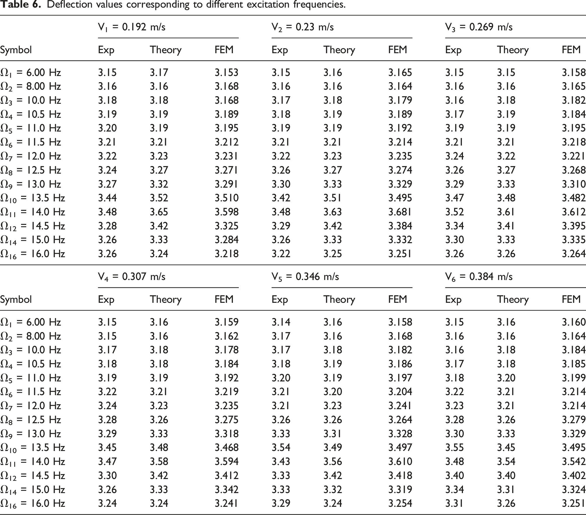
The experiment has simultaneously compared two different values, including the values of deflection and acceleration. The results are presented in Figures 9 and 10, where it can be seen that the value obtained from the deflection is much more effective than the acceleration value. The deviation of the deflection value for each excitation force status is shown in Table 6. The deflection values are a stable parameter, with little influence from external agents in better evaluating the changes in structure than the acceleration value.

From the results of Table 6 and Figure 11, the constrained frequency during the experiment will increase from 6 Hz to 14 Hz, which means that the received deflection also increases. The deflection value gradually increases up to the level of the constrained frequency and reaches the maximum level close to the beam’s level of dedicated frequency. Then, it gradually decreases. This is an important breakthrough in this research; further research may suggest levels of optimal excitation frequency that are suitable for different types of actual structures. The models of both the theory and experiment give us similar graph shapes at the levels of the respective constrained frequency, but the theoretical model will receive better results due to the mechanical modeling possessing the most perfect and optimal status.

Figure 11.

Standard deviation of deflection.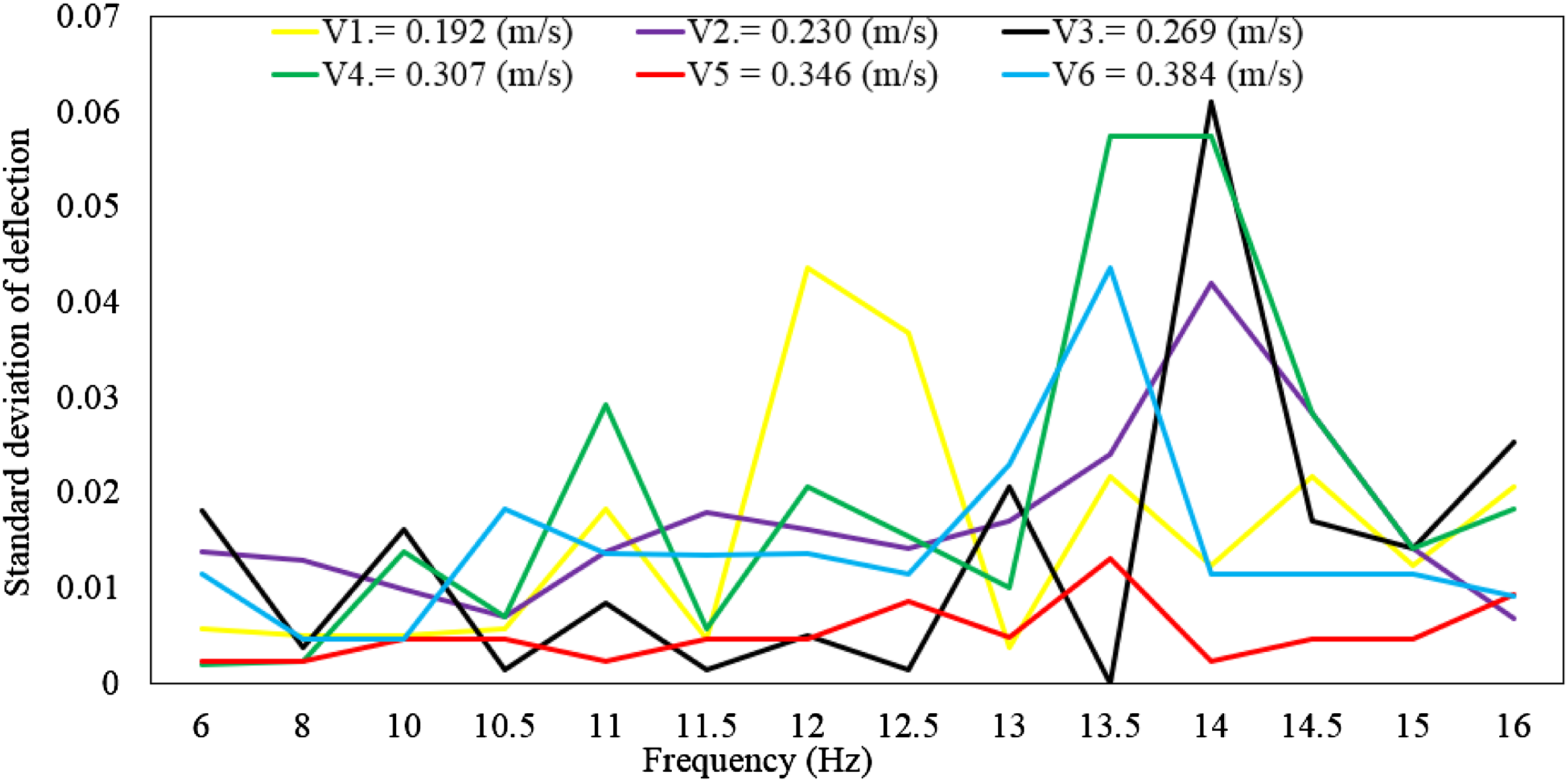

The range of deviations between measurement times compared to the average value in the case of being close to the dedicated frequency when falling into the resonance region also gives us a larger result than the levels of the remaining excitation frequency. This is a frequency region with high instability, causing many deviations during the measurement process as well as the data processing. Figures 11 and 12 show all excitation conditions; when the constrained frequency changes from 6 Hz to 12.5 Hz, we will get a small deviation result. From the frequency level 12.5 Hz–14 Hz, the deflection deviation between the theory and experiment, according to the experiment, significantly increases to reach the maximum value. When the constrained frequency exceeds 14 Hz, the deflection deviation tends to decrease gradually and is inversely proportional to the constrained frequency. Because the deflection deviation between the theory and experiment is small, we can say that the deflection values obtained from the theory and experiment are equivalent together.

Figure 12.

The deviation of theoretical deflection compared to the experiment corresponding to the excitation levels (%).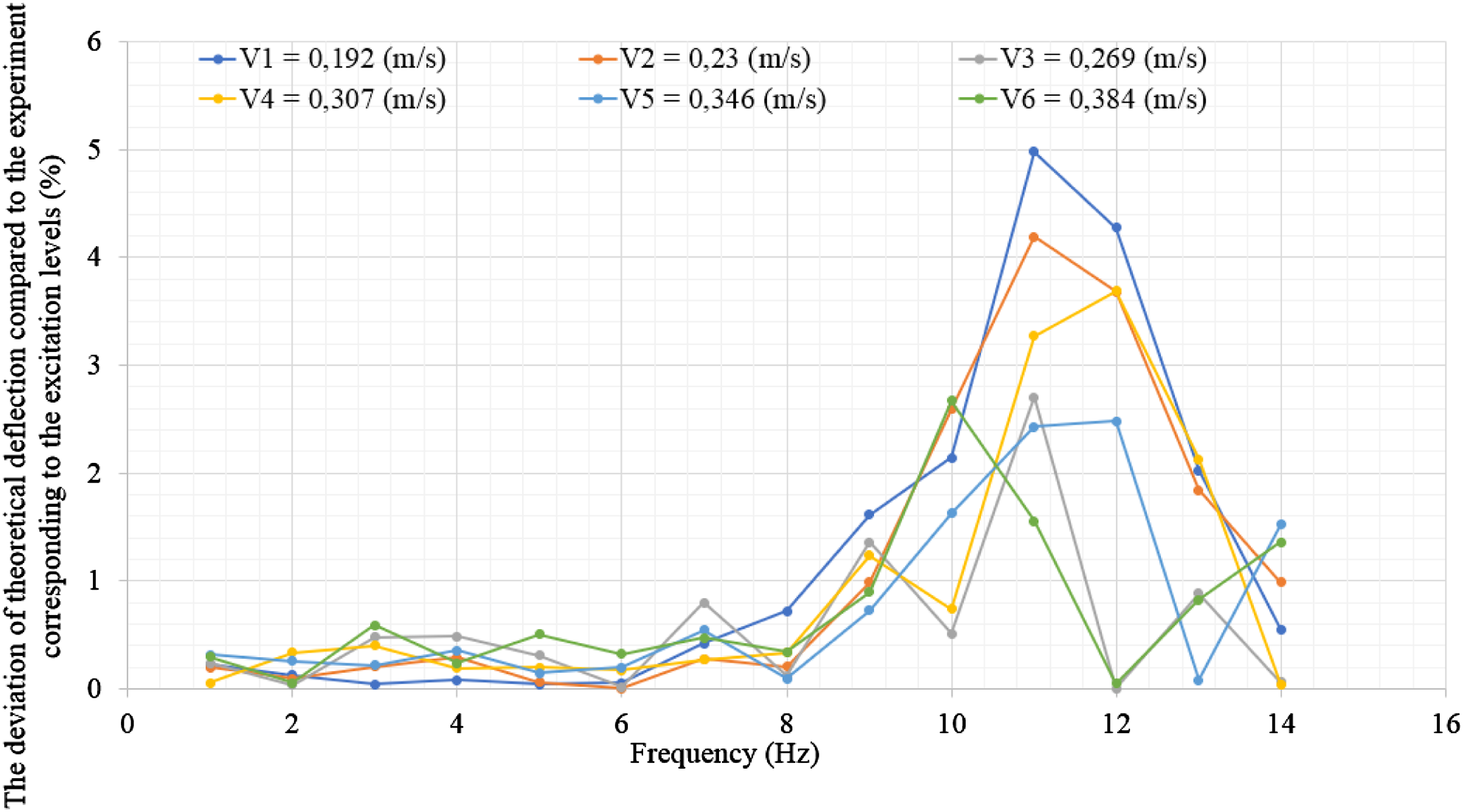

Evaluating the structure change by cumulative method

With six different velocity statuses from V₁ to V₆, the graph of the deflection signal is shown in Figure 13. Topics for which a small amount of interesting information has been shown include the following: the difference of signals according to different measurement statuses and the relationship between the measured signals and the parameters, where the structure quality has been evaluated and the next structure’s behavior and defects have been predicted. Clearly, the results of the deflection values in Section 3.1 show little change in the different experimental statuses, as shown in Figure 8. On the other hand, according to the evaluation results in Section 3.2.1, as shown in Figures 9 and 10, the deflection value according to the experiment, theory, and results simulated by FEM is always stable in many measurement statuses compared to the acceleration signal. From the above analysis results, the external impact conditions do not affect the structure, including the velocity and frequency of the excitation force. However, in the case of only performing this old evaluation method, much information is omitted and left unexploited. Therefore, the manuscript proposes a method to identify the existence of defects in the structure to evaluate changes in the deflection signal over time. The manuscript proposes using the evaluation model through the method of accumulating deflection values over time and building their cumulative circle. The results for the application of the evaluation method proposed in this manuscript are shown in Figure 13.

Figure 13.

Cumulative circle of deflection amplitudes in six statuses of different experimental velocities.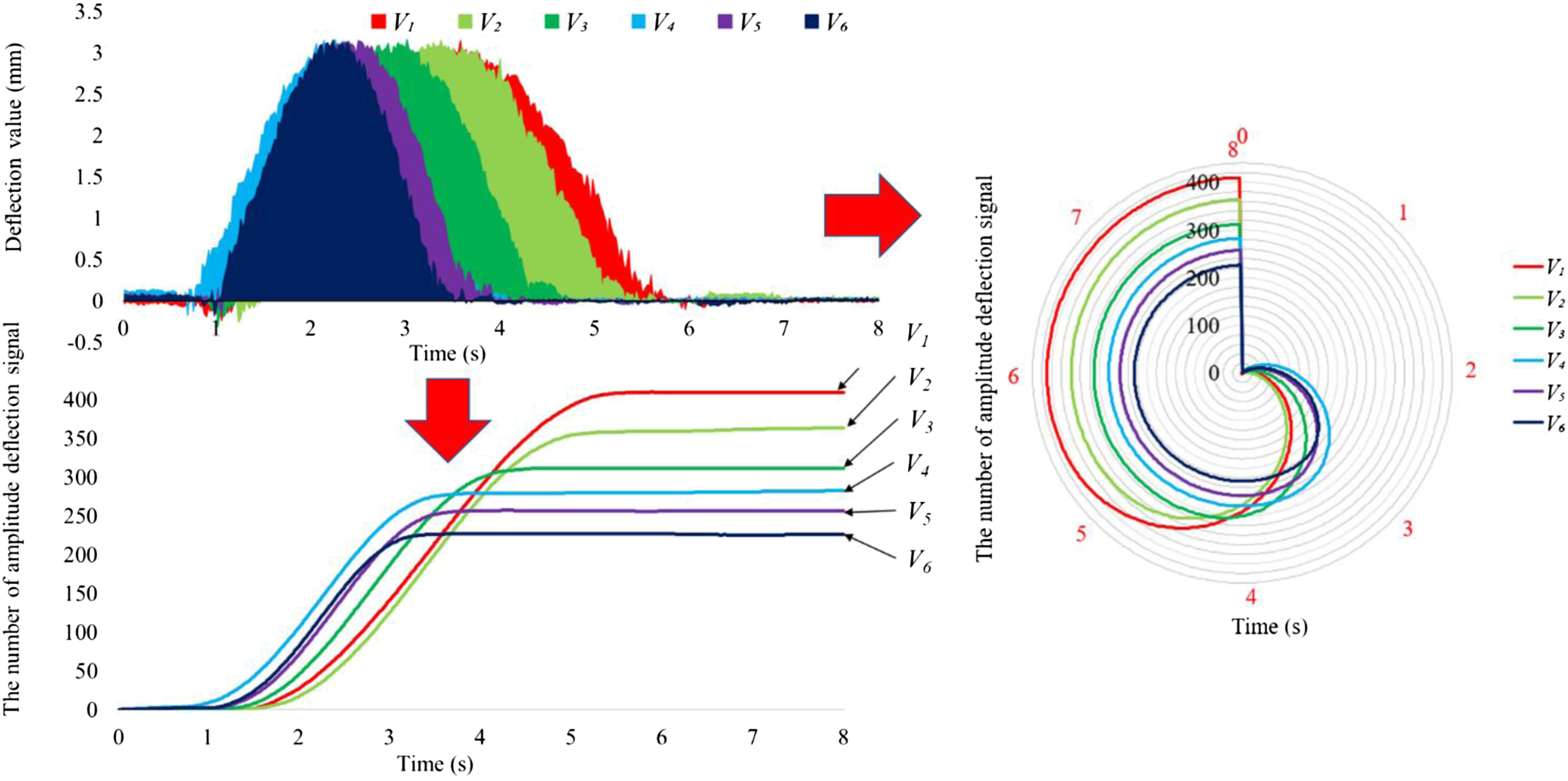

The accumulation of deflection values allows us to identify very sharp differences in the conditions of the changed experiment. For the case in which the velocity statuses have changed from V₁ to V₆, when the model moves at a high speed of V_6, the cumulative function will be much lower than at the low velocity of V₁. This observation reveals many new points because most of the previous research and the analysis from the model in Section 3.1 have always assumed that velocity has no or little effect on the structure’s operation. From the results in Figure 13, we can see that when moving at a slow velocity, the processes of both stabilization and accumulation are much longer.

During the operation, the structure will destabilize in the second ¼ angle range and stabilize at other regions in the cumulative circle model of deflection amplitudes in six statuses of different experimental velocities. The relationship between the deflection signals and the structure quality can be understood as always stable because only after a certain duration will these values recur until the end of the working process. In other words, the structure quality is kept in a stable condition throughout the working period despite the different levels of stimulus.

The results are shown from Figures 14–17 to evaluate the changes in the cumulative function of deflection values in case defects exist in the structure. These changes correspond to the defect levels, which gradually increased from H₈ to H_24, and the changed velocity during the experiment.

Figure 14.

Cumulative model of statuses of different defects in beams at V₁. (a) Cumulative function of deflection amplitude in other defective statuses at V₁. (b) Cumulative circle of deflection amplitude in other defective statuses at V₁.

Figure 15.

Cumulative model of statuses of different defects in beams at V₂. (a) Cumulative function of deflection amplitude in other defect statuses at V_2. (b) Cumulative circle of deflection amplitude in other defect statuses at V₂.

Figure 16.

Cumulative model of statuses of different defects in beams at V₃. (a) Cumulative function of deflection amplitude in other defect statuses at V₃. (b) Cumulative circle of deflection amplitudes in other defect statuses at V₃.

Figure 17.

Cumulative model of statuses of different defects in beams at V₄. (a) Cumulative function of deflection amplitude in other defect statuses at V₄. (b) Cumulative circle of deflection amplitudes in other defect statuses at V₄.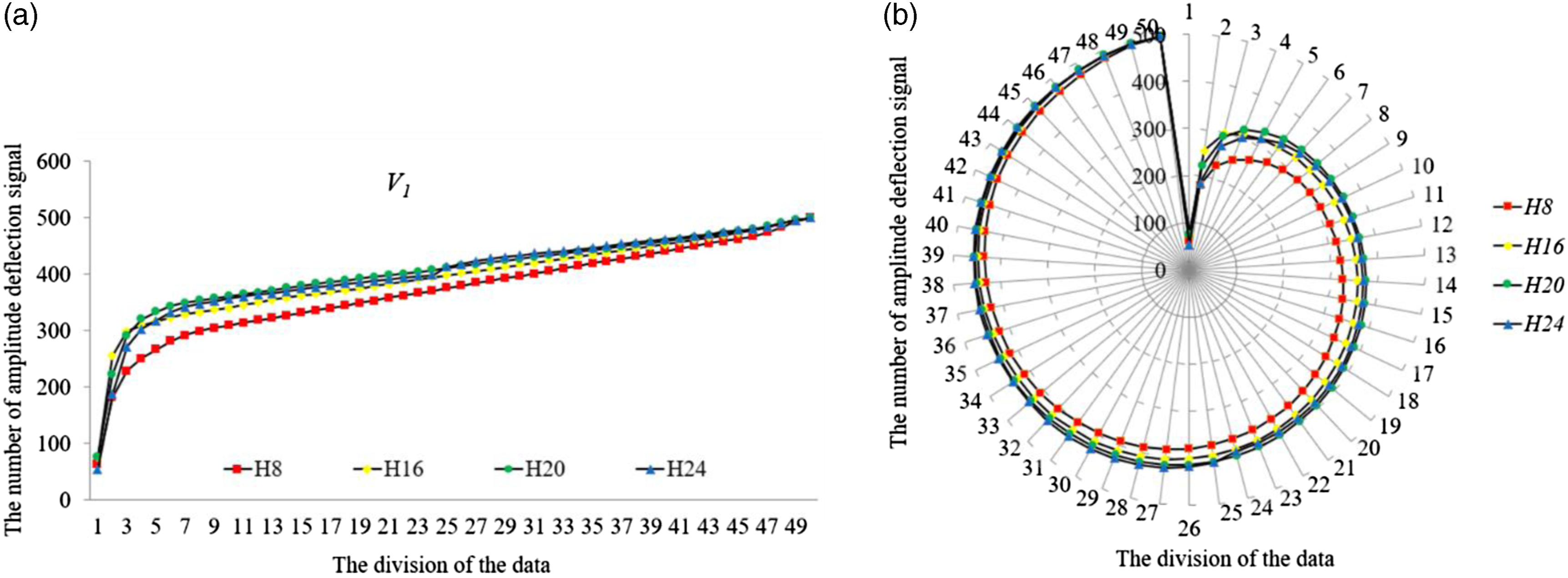

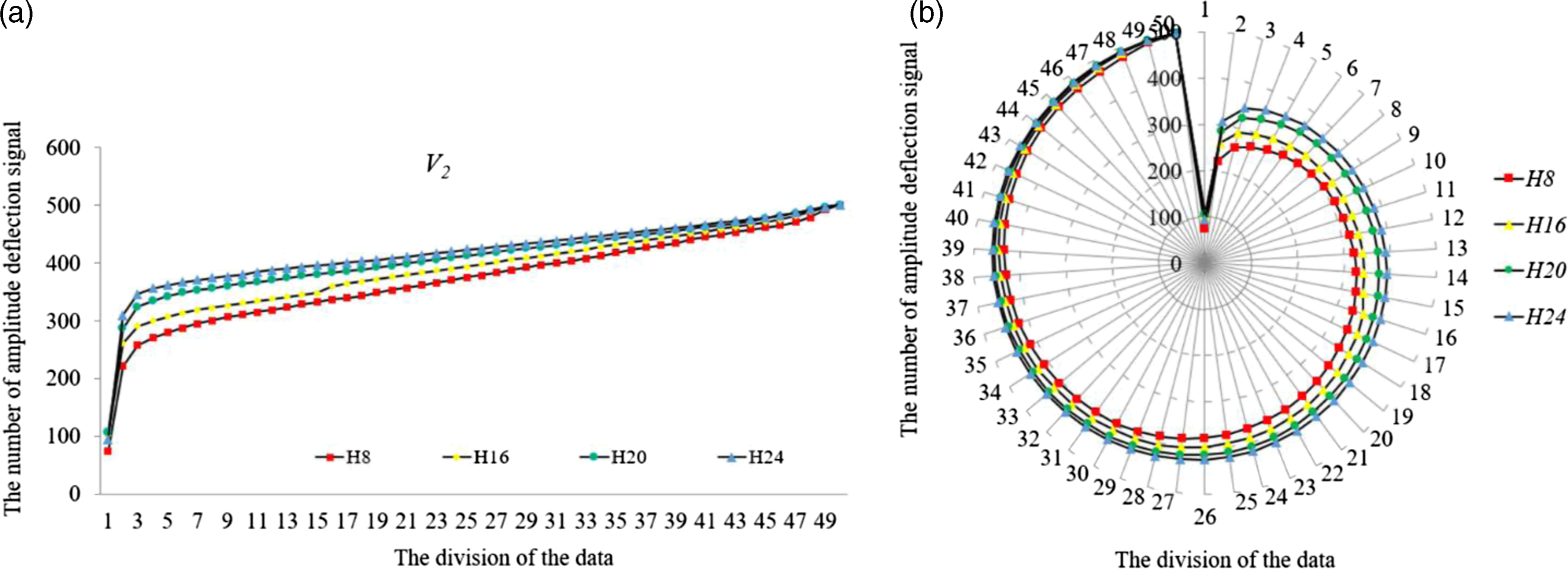
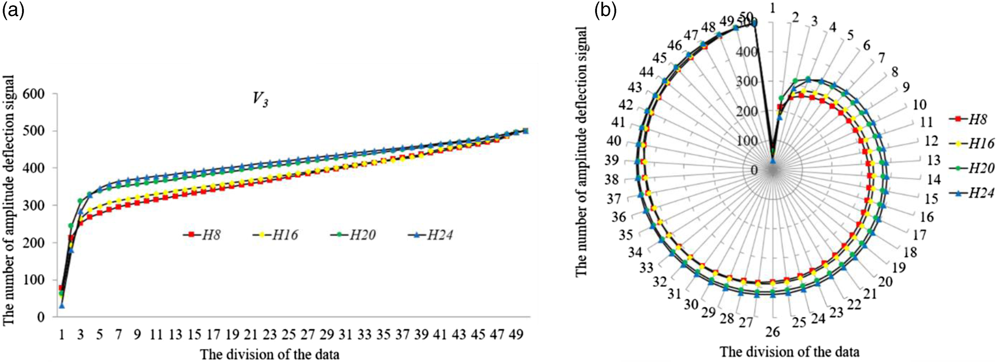
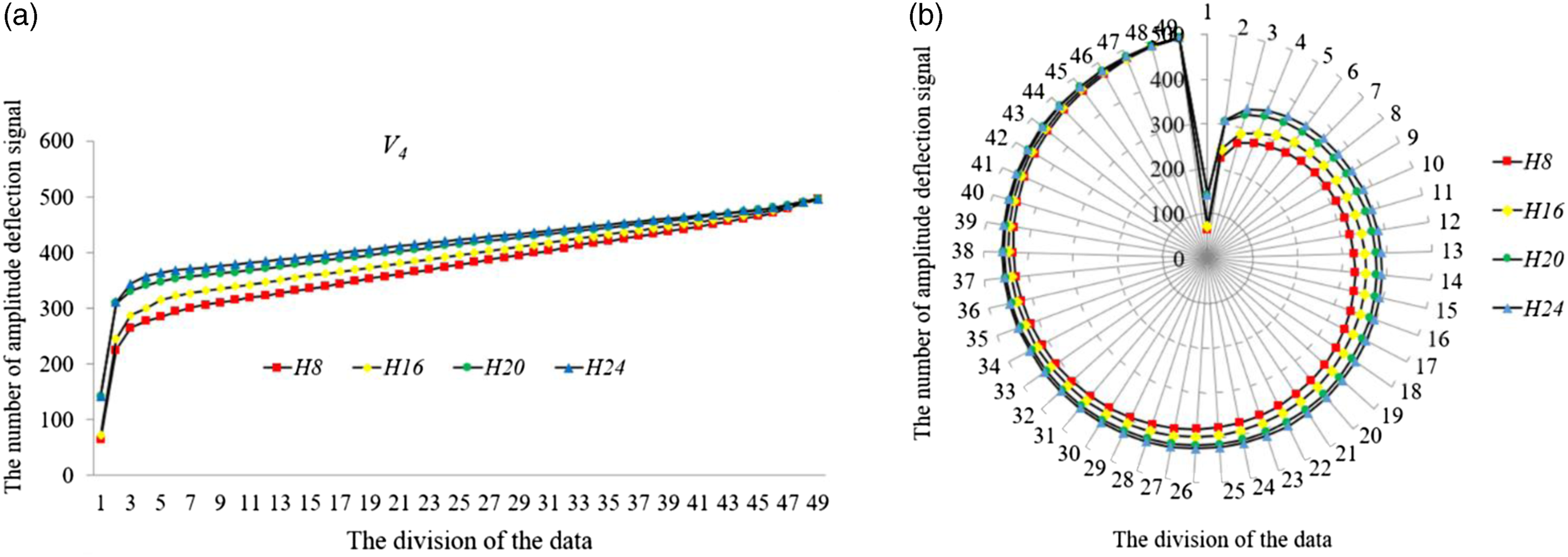
Correspondingly, progressive degrees of defects are created in the beam structure under different excitation conditions. The results from the manuscript have indicated three evaluation factors, as follows.

The regression rate of the accumulated values of deflection signals received on the beams. The lower the experimental execution velocity, the slower the regression rate, corresponding to different velocity statuses. The velocity will determine the regression rate of the obtained dataset and is demonstrated by the structure’s working capacity in case of defects being carried. However, the variation in the data’s regression speed is still small in this experimental model without being clearly shown in the statuses of different disabilities under the progressive level. This result is completely consistent with many studies,^5,8,9,44 where cuts on the beam structure were made to indicate the structure’s defect-bearing status as being completely inappropriate. Obviously, many defects still exist in the case of implementing the experiment to evaluate structural damage through the cutting model.

The degree of values that changed in the cumulative function demonstrated the difference caused by the damage to the structure. As can be seen in Figure 17, only the first defect H₈ gives the cumulative model a different status; when the defect gradually increases, this model changes for the influence of defects to be shown on the structure. The value of the cumulative function in the small defect is always within the cumulative value of the large defect at certain distances.

The results of the regression circle in the texture show the texture’s resilience. The mode of defect development in a structure mainly depends on the degree of texture restoration. If the structure is still able to recover, the defect’s degree of influence is small, and the service life of the structure can be increased. Thus, the evaluation of the results obtained through the cumulative model and the cumulative circle of deflection values can open up many different appraisals in the defect identification abacus.

Conclusions

The evaluation and identification of structures with defects through the beam structure’s signal of deflection measurement is nothing new. However, the method for evaluating and using the cumulative and circular models from the deflection measurement value has produced many new results through which many different conceptual statuses of defective structures can be evaluated. The main results obtained from this manuscript include the following.

The deflection signal is one of the important signals used by many researchers to evaluate a structure’s change. In the old evaluation method, deflection usually depended on the velocity of the moving load and the frequency of the excitation force that impacted the model with unchanged measurement results (slightly changed) in the statuses of different experiments. However, we can see through the appraisals from this manuscript that the deflection value depends considerably on the velocity as well as the force frequency. The excitation forces have the strongest influence when their values closely approach the structure’s dedicated frequency value. This can help us detect and avoid breakdowns caused by the frequency of the excitation force.

This manuscript contains proposals for evaluating the models of defective structures using the cumulative function and cumulative circle of deflection values. Based on these models, the velocity can be identified to determine the regression speed of the collected dataset, which will show the structure’s working ability in cases where it must bear the defects. Furthermore, the regression circle in the texture also demonstrates resilience in that texture. The mode of defect development in a structure depends on the degree of texture restoration.

Footnotes

Declaration of conflicting interests

The author(s) declared no potential conflicts of interest with respect to the research, authorship, and/or publication of this article.

Funding

The author(s) received no financial support for the research, authorship, and/or publication of this article.

ORCID iD

Thanh Q Nguyen

References

Hanumanthappa

. A new structural damage detection method for cantilever beam using generalized flexibility quotient difference method. J Vib Eng Technol 2022. DOI: 10.1007/s42417-022-00655-0.

Agathos

Tatsis

Vlachas

, et al. Parametric reduced order models for output-only vibration-based crack detection in shell structures. Mech Syst Signal Process 2022; 162: 108051.

Momeni

Ebrahimkhanlou

. High-dimensional data analytics in structural health monitoring and non-destructive evaluation: a review paper. Smart Mater Struct 2022; 31: 043001. DOI: 10.1088/1361-665X/ac50f4 .

Nguyen

. Detecting and evaluating defects in beams by correlation coefficients. Shock Vib 2021; 2021: 6536249.

Liu

, et al. Evaluation and prediction of material fatigue characteristics under impact loads: review and prospects. Int J Struct Integr 2022; 13: 251–277. DOI: 10.1108/IJSI-10-2021-0112 .

Salgado

PauloCruz

Ayala

. Performance of damage detection methods used in bridge structures through dynamic tests in steel beams. Am J Civ Eng 2014; 2(2): 18–26.

Nguyen

Vuong

CanhLe

, et al. A data-driven approach based on wavelet analysis and deep learning for identification of multiple-cracked beam structures under moving load. Measurement 2020; 162: 107862.

Baran

Garbatov

. Structural integrity assessment of fixed support structures for offshore wind turbines: a review. Ocean Eng 2022; 244: 110271.

Ngo

Nguyen

ThuVu

, et al. An fast Fourier transform–based correlation coefficient approach for structural damage diagnosis. Struct Health Monit 2020; 20: 2360–2375.

. Stochastic fatigue crack growth simulation of interfacial crack in bi-layered FGMs using XIGA. Comput Methods in Appl Mech Eng 2015; 84(1): 186–229.

11.

Kunin

. Stochastic model of brittle crack growth under cyclic load. Int J Pure Appl Math 2013; 84(3): 163–174.

12.

Yan

. A boundary element modeling of fatigue crack growth in a plane elastic plate. Mech Res Commun 2006; 33(4): 470–481.

13.

Belytschko

Black

. Elastic crack growth in finite elements with minimal remeshing. Int J Numer Methods Eng 1999; 45(5): 601–620.

14.

Price

Trevelyan

. Boundary element simulation of fatigue crack growth in multi-site damage. Eng Anal Bound Elem 2014; 43: 67–75.

15.

Guo

, et al. An interaction integral method for 3D curved cracks in nonhomogeneous materials with complex. Int J Solids Struct 2010; 47(16): 2178–2189.

16.

Rabczuk

Belytschko

. Cracking particles: a simplified meshfree method for arbitrary evolving cracks. Int J Numer Methods Eng 2004; 61(13): 2316–2343.

17.

Rabczuk

Belytschko

. A three dimensional large deformation meshfree method for arbitrary evolving cracks. Comput Methods in Appl Mech Eng 2007; 196(29-30): 2777–2799.

. A nite element method for crack growth without re-meshing. Int J Numer Methods Eng 1999; 46(1): 131–150.

, et al. Quasi-automatic simulation of crack propagation for 2D LEFM problems. Eng Fract Mech 1996; 55(2): 321–334.

20.

Tanaka

. Fatigue crack propagation from a crack inclined to the cyclic tensile. Eng Fract Mech 1974; 6(3): 493–507.

. A new Bernoulli–Euler beam model incorporating microstructure and surface energy effects. Zeitschrift für angewandte Mathematik und Physik 2014; 65: 393–404.

. Crack identification in vibrating beams using the energy method. J Sound Vib 2001; 224(2): 339–357.

. Beam damage detection under a moving load using random decrement technique and Savitzky–Golay filter. Sensors 2019; 20(1): 243.

24.

Kordestani

Zhang

. Direct use of the Savitzky–Golay filter to develop an output-only trend line-based damage detection method. Sensors 1983; 20(7): 2020.

, et al. Experimental and numerical investigation on the deflection behavior of pre-cracked and repaired reinforced concrete beams with fiber-reinforced polymer. Constr Build Mater 2020; 249: 118745.

, et al. Beam deflection monitoring based on a genetic algorithm using lidar data. Sensors 2020; 20(7): 2144.

27.

Domski

Zakrzewski

. Deflection of steel fiber reinforced concrete beams based on waste sand. Materials 2020; 13(2): 392.

28.

Zhang

. Statistical damage identification for bridges using ambient vibration data. Comput Struct 2007; 85(7-8): 476–485.

. Statistical analysis of online strain response and its application in fatigue assessment of a long-span steel bridge. Eng Struc 2003; 25(14): 1731–1741.

. Bridge management system and maintenance optimization for existing bridges. Comput-Aided Civ Inf 2000; 15(3): 45–55.

31.

Furuta

Watanabe

. A fuzzy expert system for damage assessment using genetic algorithms and neural networks. Microcomput Civ Eng 1996; 11(1): 37–45.

32.

Mares

Surace

. Application of genetic algorithms to identify damage in elastic structures. J Sound Vib 1996; 195(5): 195–215.

. Substructural identification using neural networks. Comput Struct 2000; 77(1): 41–52.

34.

Chang

TYP

, et al. Structural damage detection using an iterative neural network. J Intell Mater Syst Struct 2000; 11(1): 32–42.

, et al. A neural network approach for structural identification and diagnoses of a building from seismic response data. Earthq Eng Struct Dyn 2003; 32(2): 187–206.

36.

Zhu

Law

. Wavelet-based crack identication of bridge beam from operational deection time history. Int J Solids Struct 2006; 43(7-8): 2299–2317.

. Crack identication in beams using wavelet analysis. Int J Solids Struct 2003; 40(13-14): 3557–3569.

38.

Anantha Ramu

T Johnson

. Damage assessment of composite structures: a fuzzy logic integrated neural network approach. Comput Struct 1995; 57(3): 491–502.

39.

Bernal

. Load vectors for damage localization. J Eng Mech 2002; 128(1): 7–14.

40.

Sohn

Kincho

. Law, application of ritz vectors to damage detection for a grid-type bridge model. In: Proceedings of the 17th International Modal Analysis Conference, Kissimmee, FL, USA, February 1999.

41.

Sohn

Kincho

. Law, damage diagnosis using experimental ritz vectors. J Eng Mech 2001; 127(11): 1184–1193.

42.

Ball

. Stability theory for an extensible beam. J Differ Equ 1973; 14: 399–418.

43.

Nguyen

. A data-driven approach to structural health monitoring of bridge structures based on the discrete model and FFT-deep learning. J Vib Eng Technol 2021; 2021: 1–23.

44.

Nguyen

. Structural health monitoring of bridge spans using moment cumulative functions of power spectral density (MCF-PSD) and deep learning. Bridge Struct 2021; 17(1–2): 15–39.

45.

Fryba

. Vibration of solids and structures under moving loads. London, UK: Telford, 1999.

46.

Wang

. The discontinuous Galerkin finite element method for caputo-type nonlinear conservation law. Math Comput Simul 2020; 169: 51–73.

47.

Harsch

Eugster

. Finite element analysis of planar nonlinear classical beam theories. Dev nov appro nonlin solid body mech 2020; 2020: 123–157.

, A coupled finite element-element-free Galerkin method, Comput Mech 1995; 17: 186–195.

. Asymptotic decay of Fourier, laplace and other integral transforms. J Math Anal Appl 2020; 483(1): 123560.

50.

Tuan

. On the Fourier-sine and Kantorovich–Lebedev generalized convolution transforms and their applications. Ukr Math J 2020; 7(2): 302–316.

51.

Britvina

. The shift operators related to the Fourier cosine and sine transforms and visualization of their action. J Phys Conf Ser 2020; 1658: 012006.

52.

Donolato

. Analytical and numerical inversion of the Laplace–Carson transform by a differential method. Comput Phys Commun 2002; 145(2): 298–309.

, et al. Numerical inversion of the laplace–Carson transform applied to homogenization of randomly reinforced linear viscoelastic media. Comput Mech 2007; 40: 771–789.

54.

Kumar

Qureshi

. Laplace-Carson integral transform for exact solutions of non-integer order initial value problems with caputo operator. J Appl Comput Mech 2020; 19(1): 57–66.

. Duality relations of Kamal transform with laplace, laplace–Carson, Aboodh, Sumudu, Elzaki, Mohand and Sawi transforms. SN Appl Sci 2020; 2: 135.

Structural health monitoring based on the cumulative function and cumulative circle of a defective beam under a moving load

Abstract

Keywords

Introduction

Theoretical basis

Displacement model of the load-bearing beam structure

Building the signal amplitude accumulation model

Experimental model

Results and comments

Evaluating the deflection of the experimental model under the influence of a moving load as compared against the theory

Evaluating the influence of the stimulus conditions between the theory and experiment

Influence of the speed and frequency of the constraining force on deflection

Evaluating the structure change by cumulative method

Conclusions

Footnotes

Declaration of conflicting interests

Funding

ORCID iD

References