Sage Journals: Discover world-class research

Abstract

Concerns about potential health risks from infrasound exposure require objective investigation methods for the perception of infrasound by humans. Neural-network methods were applied to identify weak infrasound evoked potentials and to investigate the efficacy of these techniques. Two simple networks – a fully connected three-layer feed-forward network and a two-layer autoencoder – were designed for the analysis of electroencephalography (EEG) data recorded in response to infrasound stimuli presented. Late auditory evoked potentials (LAEPs) were detected and correlation factors between the target and the output of the networks were determined to assess the differentiation ability of the two networks. Both networks were able to differentiate infrasound evoked potentials from noise but showed different performance levels with respect to a differentiation threshold. The results can be applied to objectively identify perception events by infrasound in humans.

Keywords

Infrasound machine learning deep learning auditory evoked potentials autoencoder

Introduction

Transitioning to carbon-neutral energy production is essential for mitigating climate change and a sustainable production and life; however, renewable energy converters often produce noise specifically at low frequencies including infrasound. Serious concerns and complaints by those living in the vicinity of planned facilities often complicate the expansion and development of environmentally friendly energy production. Since objective knowledge about humans’ infrasound perception mechanisms is still limited in this field, the current debate mostly relies on assumptions; furthermore, experts are divided in their opinions as to whether infrasound has a negative impact on humans.¹

A basic but essential element of this debate is an understanding of infrasound perception mechanisms to allow a better estimation of the impact of infrasound on vulnerable anatomical structures in the human body and on processes critical for quality of life such as sleeping and leisure time. Neuroscience methods and brain imaging can play an important role^2–4 in the modelling of perception mechanisms because they focus on the processing of infrasound perception in the brain. These activities document whether infrasound commonly considered non-audible is perceived. Here, different methods such as magnetic resonance imaging (MRI)^3,4 and magnetoencephalography (MEG)⁵ have been used. Electroencephalography (EEG) is of particular interest because it involves simple detection set-ups; however, identifying related signals is difficult because the signals are weak and a reasonable signal-to-noise ratio can only be obtained via a long averaging process.⁶ Thus, EEG studies using infrasound stimuli often apply an analysis in the frequency domain. Kasprzak⁷ investigated the influence of narrow-band signals with frequencies between 4 and 8 Hz on α -waves in EEG signals. Kolesnik et al.⁸ investigated the correlation between infrasound exposure events and the time-development of various bands of EEG signals. Nagamatsu et al.⁹ used EEG data for an evaluation of the impact of wind park noise on humans. Jurado et al.⁶ evaluated the use of the brain’s frequency-following response (FFR) as an objective correlate of individual sensitivity to infrasound and determined (cervical) vestibular-evoked myogenic potentials (cVEMPs)¹⁰ in response to infrasound stimuli. In case of a time-dependent analysis, quite strong signals around a delay of 100 ms (N1) and 200 µs (P2) were expected⁵ and were clearly recognisable at audible frequencies. This raises the question as to whether it is possible to transfer knowledge of the pattern in the audible frequency range at (for example) 256 Hz into the infrasound frequency range where identifying evoked potentials is much more difficult. Methods which can exploit learned information during processing of signal patterns in EEG signal analysis help to objectively analyse results of infrasound perception studies.

A trained neural network has been used to analyse unknown data to find structures or patterns within a dataset or to classify input data into different categories.¹¹ An alternative approach is the application of unsupervised learning to reduce unintended signal contents such as noise and artefacts.^12,13 Machine learning has already been used extensively to process EEG data; here, most studies have focussed on classification or feature extraction from time data (for example, for seizure detection, sleep stage scoring and mental workload determination).^14–16 The different network configurations used were often finally adapted to specific applications via a trial-and-error methodology. Other studies have focussed on improving processing tools¹⁴ used for artefact reduction (among other tasks).¹⁷

Another motivating factor behind applying neural networks to analyse EEG data is that such data can be used to establish brain-machine interfaces. In comparison to other brain imaging methods, EEG is a simple technique for extracting information from the brain; sophisticated procedures have been established to recognise specific brain responses which can be assigned to isolated environmental input elements.¹⁸ Of particular interest in this field is, for example, the recognition of emotional reactions and the decoding of cognitive states.¹⁹

Speech recognition is a very general task with many applications which has been part of everyday life^20,21 for many years. Most speech recognition systems process time data and denoising is an essential element of this processing to which autoencoders have successfully been applied (Ref 11, section 14). In principle, the autoencoding process consists of two stages: In the first, the input data is encoded, after which a decoding system reconstitutes the (essence of the) signal and a cost function is created by comparing the input and the output. Here, it is assumed that the encoding process reduces the information of the input signal and concentrates it in the essential elements, removing unnecessary parts such as noise in the process. Autoencoders have been applied to tasks such as the analysis of seismological signals,¹² ultrasonic signal processing,¹³ EEG feature extraction²² and noise suppression.²³

In nearly all of the above discussed studies, the algorithms applied^23,24 implemented sophisticated network designs; furthermore, applying such algorithms requires expert knowledge and extensive experience. A more general deployment of this promising but difficult to create technology requires simple models and algorithms which can be used to better understand complicated experimental results. In this technical paper, simple neural-network methods are applied to identify infrasound evoked potentials and the efficacy of these networks is investigated. Two simple networks – a three-layer feed-forward fully connected network and a two-layer autoencoder – were designed to analyse EEG data recorded in response to the infrasound stimuli presented. Late auditory evoked potentials (LAEPs) were detected; here, the aim was to identify typical responses such as N1 or P2. Responses obtained at a frequency of 256 Hz were used as learning data and the qualified average was defined as a target and a reference. Correlation factors between this target and the output of the networks were determined for frequencies of 256 Hz, 64 Hz and 16 Hz; this allowed the differentiation ability of the two networks to be assessed.

Experimental set-up

EEG data acquisition

Participant information

All infrasound hearing experiments conducted to date have shown a wide distribution of all potential variables.^25,26 To limit the variability, data from only one test subject were used in this study. The approval of the local ethics committee was given under the reference 2018–1.

Stimuli

Short stimuli were presented as tone bursts. Since the period length increases with decreasing frequency, only three half-waves of a sinewave were included to limit the overall presentation time. To cover the low-frequency and infrasound frequency ranges, a stimulus at audible frequencies (256 Hz) was selected and combined with a low-frequency stimulus (64 Hz) and a stimulus in the infrasound frequency range (16 Hz). 300 stimuli were presented with a repetition rate of 1.0 s using a specially designed headphone system developed for the presentation of infrasound signals.²⁷ For this purpose, a RadioEar DD45 earphone transducer was mounted in an aluminium housing unit which had been developed in-house. This transducer was coupled to an ER3-14A ear-tip using a 50 cm sound-delivery tube containing several synthetic fibres at both ends. The test subject was awake but advised to be calm and relaxed.

EEG data acquisition

EEG signals were detected²⁸ in a vertical configuration (for discussion of LAEP see Sect 11 in 29) with a Tucker Davis system (RZ6 with an RA4PA head stage). Electrodes were positioned at both mastoids at TP 9 and TP 10 in accordance with the 10–20 electrode system.³⁰ The reference electrode was set at vertex (Cz). The 300 stimuli were presented in one batch and data were sampled with a sampling frequency of f_s = 24.4 kHz. Finally, 300 trials were extracted with a length of 500 ms starting at the moment when the electrical burst signal was generated. Note, that data of only one test person was used because of the general high inter-individual spreading of infrasound related experimental quantities. An improvement of statistical power of the experiment could only be achieved with about more than 20 test persons which is beyond the scope of this first study.

Learning data and test data preparation

Because LAEP signals are slowly varying time signals, the data could significantly be down sampled to f_sL = 122 Hz without loss of information to reduce the calculation time. The length of one trial was finally N_t = 62 points. The data of the learning set were not corrected with respect to artefacts; thus, no trial was excluded. 80% of the data obtained for a frequency of 256 Hz (240 trials) were used as learning data for the autoencoder (see Section Design of networks) and the remaining 20% formed the validation data. Note that the data at 64 and 16 Hz (preparation described below) act as test data.

The learning data for the feed-forward network comprised a combination of the data obtained at 256 Hz and the data measured when no stimulus was present, but all other EEG data acquisition parameters remained the same (zero measurement). So, the network also learned which signals do not contain LAEP-information. Although this strategy seems to deteriorate the learning data quality, it significantly improved the learning efficiency. The zero-measurement data were also prepared as described and 300 trials were available of which 80% (240 trials) were again used as learning data. These trials were randomly merged with the 240 learning trials of the 256 Hz case to obtain a final training set of 480 trials. The remaining 20% of the zero-measurement data were used as validation data to test the network’s robustness against fluctuations and high variance. To investigate the effect of reducing the variance of the data, an additional alternative data set was subsequently created by summing up 10 trials of the original data set; thus, 48 averaged trials were available as alternative learning data.

The targets were created by averaging all trials of every frequency and artefacts were corrected by hand. The mean square average deviation was calculated using Fieldtrip routines³¹ and all values with a particular deviation were excluded. In sum, about 40 trials were removed from each data set and the remaining trials were averaged to generate the targets.

Data at f = 64 Hz and f = 16 Hz were prepared in the same manner to be used as test data; 300 trials for each frequency were available as two test data sets. Visual inspection of all data (see Figure 3, red curves) revealed a clear LAEP at 256 Hz and a potential signal at 64 Hz. At the infrasound frequency of 16 Hz, the LAEP seemed to be completely overwhelmed by noise or coherent artefacts. The trials without a stimulus (zero measurement) seemed to be composed only of noise or artefact components.

Note that the learning process only applied data obtained at 256 Hz; the targets were used in the sense of ‘to meet by optimisation’ only for supervised learning. When the network is tested at the other frequencies, and for the zero-measurement data, the ‘target’ is simply a representation of the measured data and only used for investigating the performance of the network application.

Design of networks

Feed-forward network

A feed-forward network was designed for training by means of supervised learning. This network comprised three layers to allow the input and the output to have the same number of points; in this way, a time-dependent data trace could be retrieved as the time waveform of a filtered signal for analysis. The hidden layers were designed to allow a significant reduction of information to avoid overfitting. Optimising tests using a different number of layers revealed that two hidden layers were sufficient for this purpose.

Figure 1 shows the basic architecture of the network. Sizes of the matrices are given in square brackets. The number of input time points is given in the first number (row) and the number of neurons corresponds to the second number (column).

Figure 1.

Design of the feed-forward network: the first number in brackets above 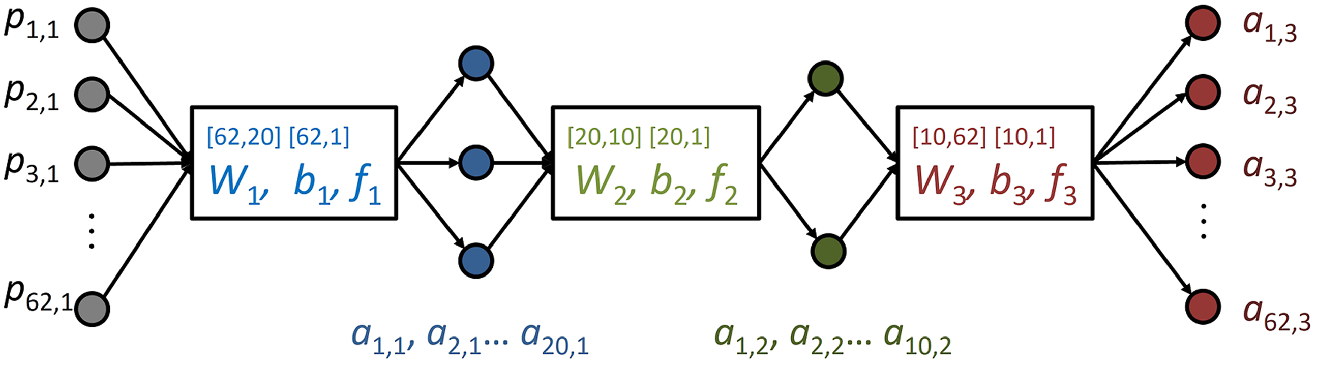W is the number of input points into the layer, while the second number is the number of output points. The numbers in brackets above b define the length of the bias vector.

Fully connecting layers (ref. 32, section 2) were realised as

a_{i} = f_{i} (W_{i} p_{i} + b_{i}) 1 \leq i \leq N_{L}

(1)

where p is the input to the network, a is the output, W is the weighting matrix, b is the bias vector, f defines the activation function and N_L is the number of layers (in this example, N_L = 3). A log-sigmoid function was chosen as the activation function in all layers and all input data were normalised between (0, 1).

The network was trained via a supervised learning rule using the trials at 256 Hz merged with the zero-measurement data (see Section Experimental setup) as learning data and their qualified average as the target t . The loss function was constructed from the mean square error

L = ‖ t - a_{N_{L}} ‖ = \sum_{i}^{N_{t}} {(t_{i} - a_{i, N_{L}})}^{2}

(2)

where N_t is the number of (time) data points.

The loss function L was minimised using a backpropagation method based on a least-mean-square optimisation via a steepest descent algorithm.³² The start values for the weightings and biases were random numbers in the interval (0,1). A momentum was introduced to reduce oscillations during calculation (ref 32, section 12), and a variable learning rate was optimised to reduce the processing time.

All calculations were carried out via a specially designed MATLAB code following the mathematical formulation of the problem by Hagan et al.³² No toolbox subroutines were used to allow the properties of the calculation and the script design to be better understood.

Autoencoder

An autoencoder with only two layers (N_L = 2) was designed (Figure 2); decoding and encoding took place with only one layer each. Fully connected layers as defined in equation (1) were used. The number of neurons in the hidden layer was varied; the correlation between the network output p and the target t of the validation data was maximised as a design criterion. Finally, the number of neurons in the first layer was set to 10.

Figure 2.

Network design of the autoencoder network: the first number in brackets above 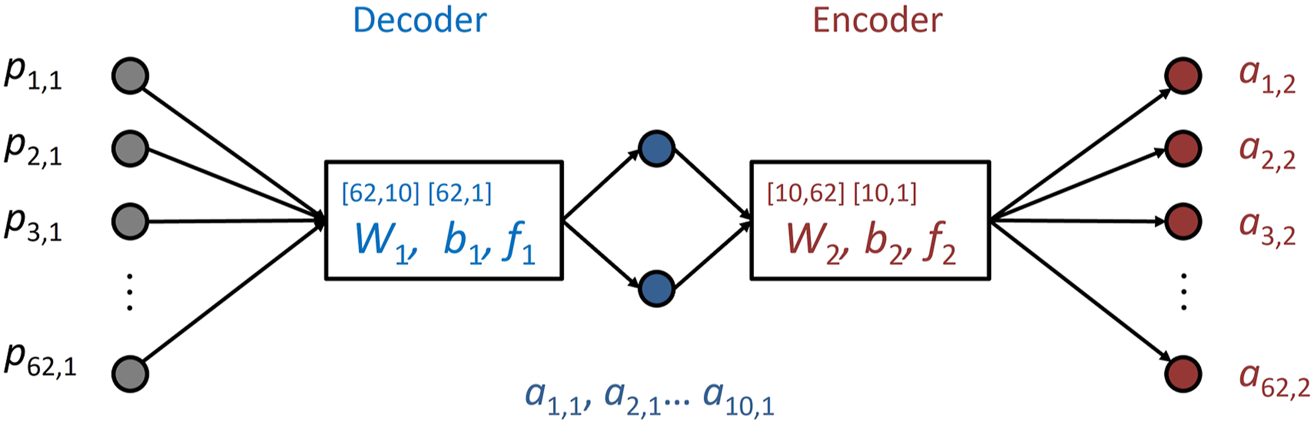W is the number of input points into the layer, while the second number is the number of output points, which is equal to the number of neurons in the layer. The numbers in brackets above b define the length of the bias vector.

The weightings in the decoding and encoding layer were independent; to increase the degrees of freedom, no coupling via transposing of the weighting matrix or bias took place.

The loss function compared the input and the output of the network. Here, several different loss functions were considered – for example, a loss function based on the Kullback–Leibler divergence¹² or on cross entropy.¹³ However, the best results were obtained via the following simple mean-square-error concept

L = ‖ p - a_{N_{L}} ‖ = \sum_{i}^{N_{t}} {(p_{i} - a_{i, N_{L}})}^{2} .

(3)

As in the case of the feed-forward network, the loss function was minimised using a backpropagation method using random start values. Several stopping criteria for the loss function were investigated (ref 32, section 17). A specified limit L_lim was defined and the moment at which the performance improvement became small was determined. However, the best results were obtained with a fixed number of cycles and by observing the improvement in the performance during convergence.

Analysis of network output

To investigate the efficacy of a neural-network analysis of time-dependent data, qualitative means are often applied because they allow N1 and P2 responses to be indicated clearly – for example, via visual inspection. However, to allow a more quantitative analysis to be performed, the similarity between the network outputs and the target traces at 256 Hz was investigated as a representation of a true LAEP signal. The correlation coefficient which describes the linear dependence between two signals can give a quantitative measure of how accurately the network can identify an LAEP in the test data.

The correlation coefficient between both data traces was calculated using the standard MATLAB routine. The correlation coefficient between the network output and the target values, calculated as the qualified averages of all trials per frequency, was determined to assess the learning process. The data given in Figure 5 consist of average values obtained from five independent runs of creating network weightings and biases using different random initial values.

Results

Feed-forward network

The feed-forward network was applied to the validation data, the two test data sets and the zero measurement. For all data, high correlation between the target at 256 Hz (as the LAEP signal) and the network output was obtained. Unfortunately, this was also the case for the zero measurement, thus clearly indicating an overfitting of the network. The network ‘learned’ to find the LAEP for every signal form, including incoherent noise.

To reduce the variance of the learning data, pre-averaging was carried out and the training was repeated with the alternative data set containing 48 trials. Then, the network was applied to the test data and the zero measurement. Figure 3 shows the results obtained. Visual inspection of the targets (red lines) revealed a clear LAEP at 256 Hz for the validation data and a potential signal at 64 Hz. At the infrasound frequency of 16 Hz, the LAEP seems to be completely overwhelmed by noise or coherent artefacts. For the validation data, the network clearly identifies an LAEP, while for the 64 Hz test data, an appropriate signal can be seen. For 16 Hz, an LAEP is recognisable, whereas for the zero measurement, the LEAP is lost, as expected. The similarity to the target, as represented by the averaged trials specific to each frequency, decreases with decreasing frequency; however, for the zero measurement, it increases again significantly. Here, the network seems to recognise the ‘other’ signal type it learned, which represents the noise and the coherent disturbances inherent to the EEG system.

Figure 3.

Network output (in blue) of the feed-forward network and targets (in red) for four data cases with pre-averaging (10 times); upper left: validation data at 256 Hz; upper right: test data at 64 Hz; lower left: test data at 16 Hz; lower right: zero measurement; on all horizontal axes, the time values start with the start of the stimulus, while the vertical axis represents the normalised EEG electrode voltage at TP9.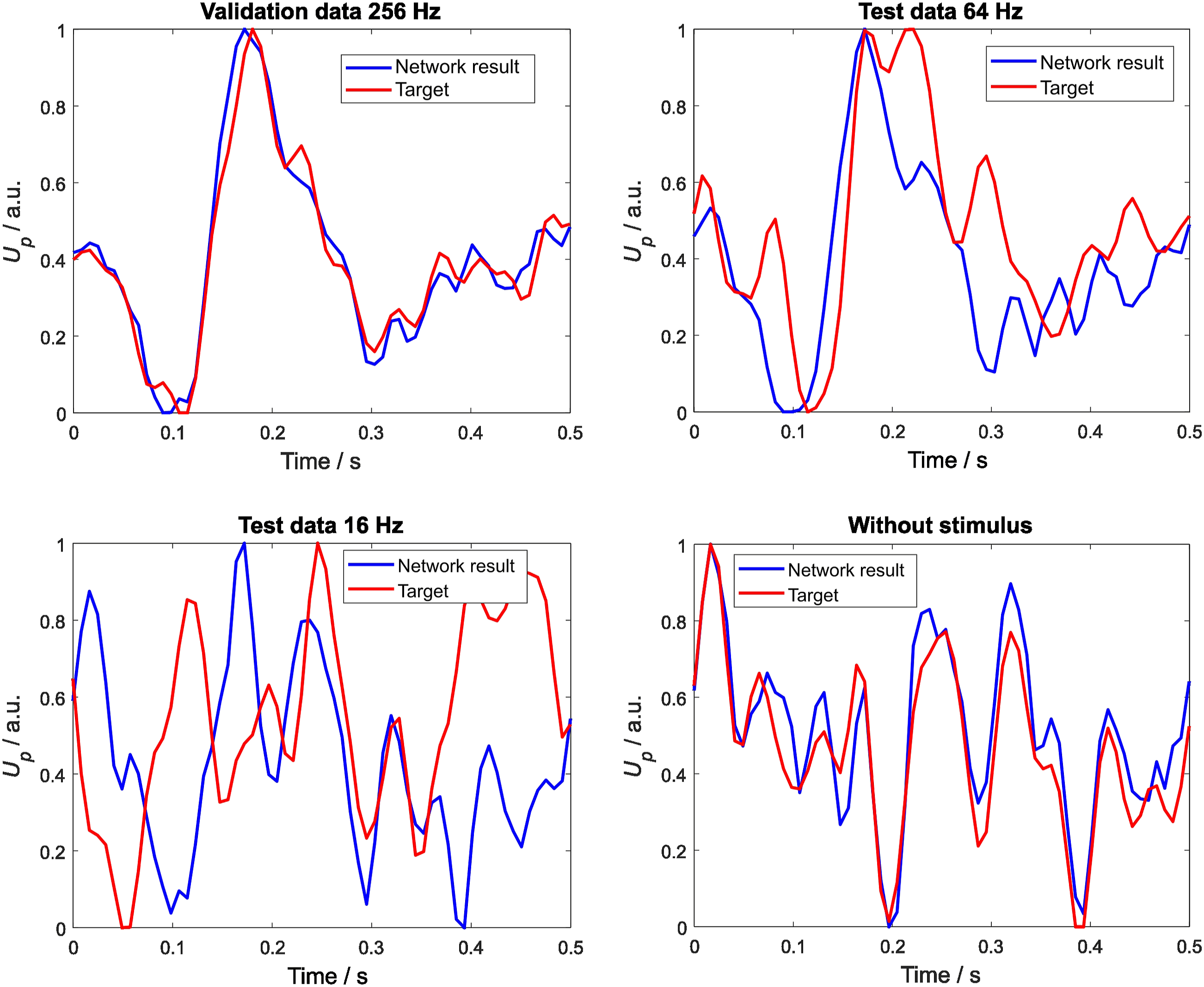

Autoencoder

The autoencoder network was applied to a data arrangement which was similar to the feed-forward network but whose first step involved no pre-averaging using 240 training trials. Note that, in this case, only data with stimulus presentation were used. As shown in Figure 4 in the validation data, a clear LAEP signal can be identified, which also holds for the 64 Hz test data. Inspection of the 16 Hz test data no longer reveals an LAEP structure for the network output, while for the zero measurement, a structured signal cannot be found. In contrast to the feed-forward results, no obvious correlation to the target (averaged values) of the noise data was observed for the zero measurement.

Figure 4.

Network output (in blue) of the autoencoder and targets (in red) for four data cases without pre-averaging; upper left: validation data at 256 Hz; upper right: test data at 64 Hz; lower left: test data at 16 Hz; lower right: zero measurement; at all horizontal axes, time values start with the start of the stimulus; the vertical axis represents the normalised EEG electrode voltage at TP9.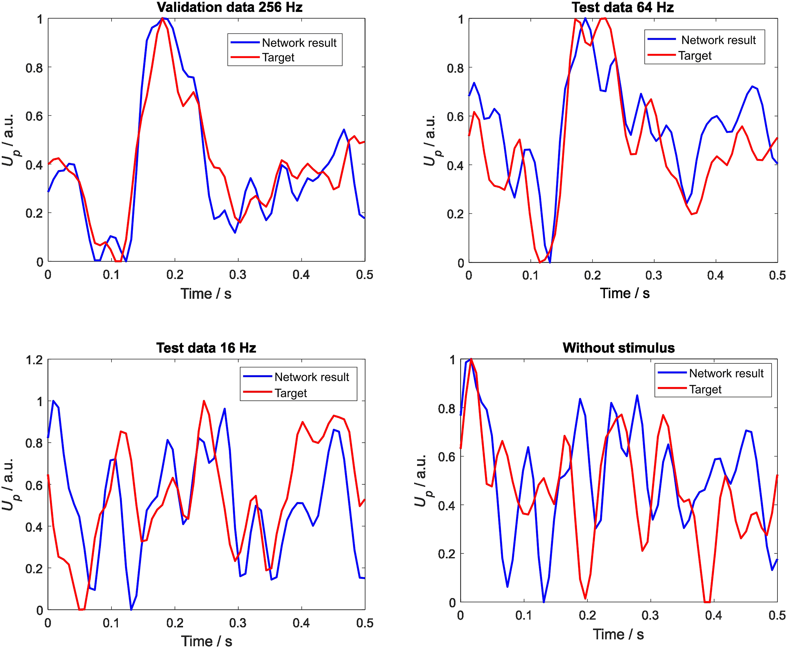

To test the dependence of the network performance on the variance of the data, a similar calculation was carried out with a pre-averaging of 10 times using the alternative data set (no figure). The differences between the network outputs of the four cases decreased (see Section Correlation analysis for performance evaluation), which can be interpreted as a decreased differentiation ability of the network.

Correlation analysis for performance evaluation

Figure 5 summarises the correlation coefficients for the various configurations calculated. The circles give the values for the autoencoder without pre-averaging. Starting from nearly perfect congruence for the validation data, the correlation coefficient decreases for 64 Hz and further for 16 Hz. There is nearly no difference between 16 Hz and the zero measurement. In contrast to this behaviour, a pre-averaging (squares) strongly reduces this decrease and only slight changes in the correlation coefficients are observed for this case.

Figure 5.

Correlation coefficients for various configurations; circle: autoencoder network output with target 256 Hz without pre-averaging; square: autoencoder network output with target 256 Hz with pre-averaging; triangle: feed-forward network output with target 256 Hz with pre-averaging; star: feed-forward network output with average value of test data with pre-averaging.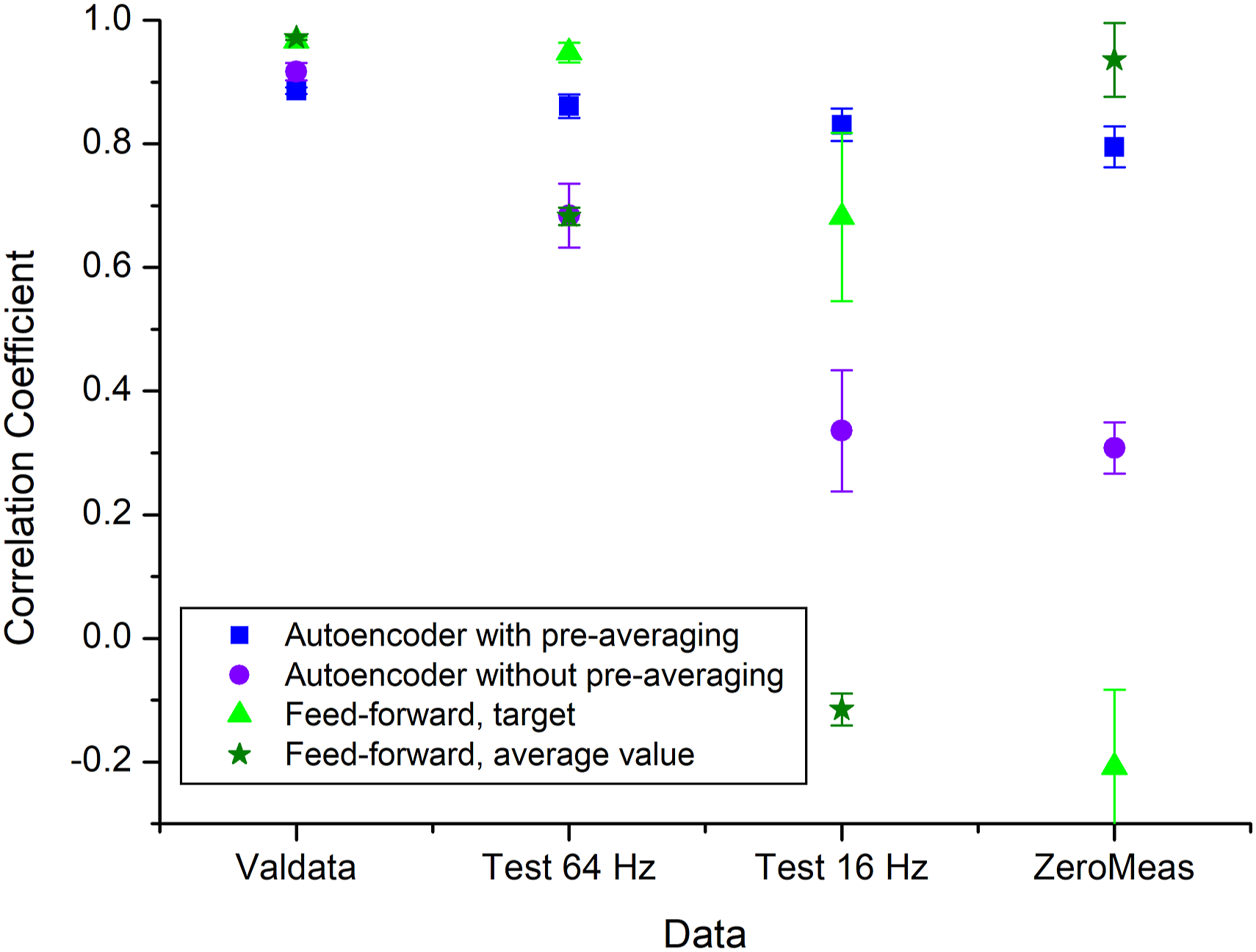

The feed-forward network shows nearly the same correlation values for the validation data and for 64 Hz; however, for 16 Hz and for the zero measurement, a strong decrease can be observed. The correlation between the feed-forward network output and the target (average values), on the other hand, follows a U-shaped curve. For the zero measurement, the correlation increases, and the network output nearly reproduces the average value of the zero measurement.

Discussion and conclusions

Two different networks representing two learning principles were applied to acoustically evoked potentials produced via an acoustic stimulus with low frequencies and one infrasound frequency. Here, the aim was to identify an LAEP signal for which the time signal could be reproduced. Both networks identified signals correctly and distinguished them from a noisy zero-measurement obtained under identical acquisition conditions but without a stimulus. However, the differentiation thresholds were different for both networks and showed general differences in functioning. The autoencoder did not differentiate between the 16 Hz test data case and the zero measurement, but the feed-forward network did not distinguish between the validation data and the 64 Hz test case. The differentiation threshold is strongly dependent on the parameters which seemed to be specific to the network.

Pre-averaging the data reduced the differences in correlation coefficients of the four data cases in the autoencoder. This can be interpreted as a loss in the differentiation ability of the network. In principle, the autoencoder gains information from the noise and its qualitative difference to coherent signal contributions. This feature relate to the applied unsupervised learning process which associates examples using the data structure or property information.^11,33 In contrast, the feed-forward model trained via supervised learning is sensitive to the amount of variance; only a low level of noise is tolerated for an acceptable differentiation ability of the network. In this sense, both networks used in this paper are complementary; the analysis of the application of both networks to data can help to set important parameters of network design to appropriate values. This is particularly useful for the final output question concerning whether an LAEP is present or not. It would be useful to define a differentiation threshold and a strategy to find such a threshold could be to optimise the signal-to-noise ratio in combination with the number of neurons in the network to bring the differentiation threshold of both types of networks to one level. This could be used as a quality assessment strategy to ensure the correct prediction of an LAEP in a signal.

Based on the properties of the learning process, it can also be observed that the feed-forward network reproduces the target (average of all trials) in case of the zero measurement. Because the zero-measurement data comprise 50% of the learning data, this target is one of the learning goals. The network reduces the variability of the data by focussing on the main properties of the signal which seem to be reflected by the average value. This can also be interpreted as a reduction in degrees of freedom. In contrast, the autoencoder does not extract the average of the zero measurement, as can be expected from unsupervised learning principles; furthermore, the network suppresses the noise. This process revealed that coherent unwanted contributions were present as artefacts in the EEG system; neural networks were applied to reduce and identify artefacts.^17,34

The amount of data was limited for this experiment, which was the first of its kind. It was not possible to investigate what amount of learning data was necessary to achieve a sufficient differentiation ability of the networks. One reason for this was the fact that obtaining data at infrasound frequencies was very time-consuming. Since the amount of time necessary for this data acquisition increases with decreasing wavelengths, long measurement times were necessary, leading to long session times for the test subjects.

During the design phase, several parameters were optimised. The numbers of the neurons of the hidden layers were varied and the correlation between the network output and the target for the validation data was maximised as a design criterion. The stopping criteria for the iteration number influenced the output results and a strong dependence of the convergence on limits L_lim was found. Setting a maximum number of iterations provided extremely stable and reliable results when the performance improvement became low. The situation was not significantly improved by introducing sparsity means such as the Kullback–Leibler divergence nor by limiting (i.e. minimising) the weighting matrix norm.^11,13 However, a careful and systematic quantitative investigation of the impact of sparsity means was not carried out and is left to further studies.

The aim of this article was to reproduce time signals to allow a comprehensive evaluation of the network. This, however, complicated the task of creating a network; in future, it may be easier to design a network which can handle pure classification tasks such as decisions on whether an LAEP exists as well as parameters or features such as MNN recognition. This, in turn, will allow a more broadly applicable network to be designed, including a combination of convolutional or recurrent network elements. However, one drawback is that the observation of the time signals allowed a better judgement of the network output and the processes taking place within the network. Ideally, future studies should also have more data available for supervised learning.

It can be concluded that neural networks can help to identify highly concealed auditory evoked potentials. Networks based on both supervised and unsupervised learning can be applied and provide complementary results. The comparison of network outputs can provide criteria for parameter settings and for the differentiation threshold required for a reliable prediction of evoked potentials. Further development of network designs can help improve the sensitivity necessary to allow results to be classified unambiguously and to reproduce time-dependent signals.

Footnotes

Acknowledgements

The author is very grateful to Marion Bug and Sven Vollbort for contributing the EEG raw data and to Marvin Rust for careful reading of the manuscript and valuable discussion.

Declaration of conflicting interests

The author(s) declared no potential conflicts of interest with respect to the research, authorship, and/or publication of this article.

Funding

The author(s) received no financial support for the research, authorship, and/or publication of this article.

ORCID iD

Christian Koch

References

Hessler

Leventhall

Schomer

, et al. Health effects from wind turbine low frequency noise and infrasound do wind turbines make people sick? that is the issue. Sound and Vibration 2017; 51: 34–44.

Koch

. Hearing beyond the limit: measurement, perception and impact of infrasound and ultrasonic noise, www.icben.org/2017/ICBEN2017Papers/Keynote02_Koch_4163.pdf (2017, accessed 20 June 2017).

Weichenberger

Bauer

Kühler

, et al. Altered cortical and subcortical connectivity due to infrasound administered near the hearing threshold—evidence from fMRI. PLoS One 2017; 12: e0174420. http://journals.plos.org/plosone/article?id=10.1371/journal.pone.0174420

Behler

Uppenkamp

. Activation in human auditory cortex in relation to the loudness and unpleasantness of low-frequency and infrasound stimuli. PLoS One 2020; 15: 1–20.

Bauer

Sander-Thömmes

Ihlenfeld

, et al. Investigation of perception at infrasound frequencies by functional magnetic resonance imaging (fMRI) and magnetoencephalography (MEG), http://www.iiav.org/archives_icsv/2015_icsv22/content/papers/papers/full_paper_257_20150428151356809.pdf (2015, accessed 14 July 2015).

Jurado

Marquardt

. Brain’s frequency following responses to low-frequency and infrasound. Arch Acoust 2020; 45: 313–319, https://journals.pan.pl/content/116321/pdf/aoa.2020.133151.pdf

Kasprzak

. The effect of the narrow-band noise in the range 4-8 Hz on the Alpha waves in the EEG signal. Acta Physica Pol A 2013; 123: 980–983.

Kolesnik

Pobachenko

Solov’yov

. Estimation of contingency of parameters of human EEG and background infrasonic vibrations of pressure revealed in monitoring studies. Izv Atmos Ocean Phys 2013; 49: 812–818.

Nagamatsu

Yamamoto

. Influence evaluation of infrasound by using both of biological information and infrasound sensors in the vicinity of wind turbine facilities, https://core.ac.uk/display/237021274 (2019, accessed 10 September 2019).

10.

Jurado

Marquardt

. On the Effectiveness of airborne infrasound in eliciting vestibular-evoked myogenic responses. J Low Freq Noise Vib Act Control 2019; 39: 3–16.

11.

Goodfellow

Bengio

Courville

. Deep Learning. Massachusetts USA: MIT Press, 2016.

12.

Chen

Zhang

Bai

, et al. Improving the signal‐to‐noise ratio of seismological datasets by unsupervised machine learning. Seismol Res Lett 2019; 90: 1552–1564.

13.

Gao

Chen

, et al. Ultrasonic signal denoising based on autoencoder. Rev Sci Instrum 2020; 91: 45104.

14.

Roy

Banville

Albuquerque

, et al. Deep learning-based electroencephalography analysis: a systematic review. J Neural Eng 2019; 16: 51001.

15.

Craik

Contreras-Vidal

. Deep learning for electroencephalogram (EEG) classification tasks: a review. J Neural Eng 2019; 16: 31001.

16.

Moinnereau

M-A

Brienne

Brodeur

, et al. Classification of auditory stimuli from eeg signals with a regulated recurrent neural network reservoir, 2018, https://arxiv.org/abs/1804.10322

17.

Selvan

Srinivasan

. Removal of ocular artifacts from EEG using an efficient neural network based adaptive filtering technique. IEEE Signal Process Lett 1999; 6: 330–332.

18.

Müller

K-R

Tangermann

Dornhege

, et al. Machine learning for real-time single-trial EEG-analysis: from brain-computer interfacing to mental state monitoring. J Neurosci Methods 2008; 167: 82–90.

19.

Zafar

Dass

Malik

. Electroencephalogram-based decoding cognitive states using convolutional neural network and likelihood ratio based score fusion. PLoS One 2017; 12: e0178410.

20.

Gaikwad

Gawali

Yannawar

. A review on speech recognition technique. IJCA 2010; 10: 16–24.

21.

Nassif

Shahin

Attili

, et al. Speech recognition using deep neural networks: a systematic review. IEEE Access 2019; 7: 19143–19165.

22.

Vařeka

Mautner

. Stacked autoencoders for the P300 component detection. Front Neurosci 2017; 11: 302.

23.

Wen

Zhang

. Deep convolution neural network and autoencoders-based unsupervised feature learning of EEG signals. IEEE Access 2018; 6: 25399–25410.

24.

Cecotti

Graser

. Convolutional neural networks for P300 detection with application to brain-computer interfaces. IEEE Trans Pattern Anal Mach Intell 2011; 33: 433–445.

25.

Kuehler

Fedtke

Hensel

. Infrasonic and low-frequency insert earphone hearing threshold. J Acoust Soc Am 2015; 137: EL347–EL353.

26.

Burke

Uppenkamp

Koch

. A psychoacoustical study to investigate the perceived unpleasantness of infrasound combined with audio-frequency sound. Acta Acust 2020; 4: 20.

27.

Friedrich

Joost

Fedtke

, et al. Spectral integration of infrasound at threshold. J Acoust Soc Am 2020; 147: EL259.

28.

Picton

Lins

Scherg

. The recording and analysis of event-related potentials. In: Boller

Grafman

(eds) Handbook of Neurophysiology. Amsterdam, Netherlands: Elsevier, 1995, pp. 3–73.

29.

Picton

. Human auditory evoked potentials. San Diego, California, USA: Plural Publishing, 2011.

30.

Klem

Lüders

Jasper

, et al. The ten-twenty electrode system of the international federation. The international federation of clinical neurophysiology. Electroencephalogr Clin Neurophysiol Suppl 1999; 52: 3–6.

31.

Oostenveld

Fries

Maris

, et al. FieldTrip: open source software for advanced analysis of MEG, EEG, and invasive electrophysiological data. Comput Intell Neurosci 2011; 2011: 156896.

32.

Hagan

Demuth

Beale

, et al. Neural network design. 2nd ed. Oklahoma: Martin T.Hangan, 2014.

33.

Roch

Gerstoft

Bozena

, et al. How machine learning contributes to solve acoustical problems-marie a roch, peter gerstoft, bozena kostek, and zoi-heleni michalopoulou. Acoust Today 2021; 17: 48–56,

34.

Phadikar

Sinha

Ghosh

. Automatic EEG eyeblink artefact identification and removal technique using independent component analysis in combination with support vector machines and denoising autoencoder. IET Signal Process 2020; 14: 396–405.

A basic identification of late auditory evoked potentials at infrasound frequencies: Support via neural network–based signal processing

Abstract

Keywords

Introduction

Experimental set-up

EEG data acquisition

Participant information

Stimuli

EEG data acquisition

Learning data and test data preparation

Design of networks

Feed-forward network

Autoencoder

Analysis of network output

Results

Feed-forward network

Autoencoder

Correlation analysis for performance evaluation

Discussion and conclusions

Footnotes

Acknowledgements

Declaration of conflicting interests

Funding

ORCID iD

References