Estimated the frequencies of a coupled damped nonlinear oscillator with the non-Perturbative method

Abstract

The current article is concerned with a comprehensive investigation of achieving the simplest solution of non-conservative coupled nonlinear forced oscillators. The article mainly depends on a non-perturbative method. It depends on yielding an equivalent linear system. The advantage of this linear system is that its coefficients are easily computed and that they include the effects of the original nonlinear coefficients. This linearization approach allows achieving quasi-exact solutions even in the presence of periodic forces. The relationships of frequencies with amplitudes are easily established. The analytical solution so yielded may serve as a basis for a qualitative understanding of the actual behavior of the coupled nonlinear oscillators. Additionally, numerical calculations are carried out graphically to address the validation of the new approach and to further illustrate the effectiveness and convenience of the method. The results are compared with the exact numerical solutions which show perfect accuracy. The method can be easily extended to other nonlinear systems and can therefore be exceedingly applicable in engineering and other sciences.

Introduction

Many of the problems in physical, mechanical, and aeronautical technology and even in tectonic applications are mostly nonlinear. The main part of the nonlinear dynamical model is fundamentally composed of a group of differential equations and auxiliary conditions for formulation processes. ¹ Nonlinear oscillation problems are common in physical science, mechanical structures, and other kinds of mathematical sciences. Most real systems are constituted by nonlinear differential equations which are significant issues in mechanical constructs, mathematical physics, and engineering. The forced damping Duffing oscillator is a familiar model for many nonlinear phenomena in science, mathematics, and engineering. The growing interest in this oscillator is due to the diversity of its physics applications given that it is isomorphic with other significant systems of physics and engineering.

Coupled nonlinear oscillators represent an excellent scope for understanding the several complex convergent dynamics that impulsively arise in real-life systems.^2–4 A prime example is the coupled damping oscillations which have been prevalent in diverse areas of science and technology. ⁵ The topic of coupled nonlinear oscillators as well as their relevance to physical and engineering applications on the one hand, and their mathematical structure on the other hand have drawn considerable attention both from the physics, engineering, and mathematics communities. These systems are significant in engineering because several practical engineering constituents consist of vibrating systems that can be compressed using oscillator systems such as elastic beams are confirmed by two springs or mass-on-moving belts or nonlinear pendulum and vibration of a chipping machine. ⁶

Nonlinear vibration is an inveterate phenomenon in rotating machinery. The main purpose of rotating machinery vibrations is the rotor disparity, the coupling imbalances, and the don between the rotating parts and the stator. Therefore, vibration analysis and control have received major attention in the last few years. Great efforts have been made to mitigate vibrations in rotating machines.^7,8 In general, it is difficult to get the exact solution for strongly nonlinear high-dimensional dynamic systems. Hence, the analytical inexact solution of the nonlinear problem has become the subject of research for many scholars in recent years.

Solving governing equations and limiting existing exact solutions have been among the most time-consuming and difficult issues faced by researchers in vibration problems. There are several methods used to solve nonlinear differential equations. Among the most widely used methods are the homotopy perturbation method,^9–13 the effectiveness of the homotopy perturbation method for strongly nonlinear oscillators is disccused by He et al. ¹⁴ A generalized Duffing oscillator is adopted to elucidate the solving process step by step, and a nonlinear frequency-amplitude relationship is obtained with a relative error of 0.91%. In addition, the variational iteration method,^15-16 and the harmonic balance method.^17–19 Often, such traditional perturbation methods are not feasible in the case of the non-conservative oscillation, in which case it must deal with new methods.^20–22

One of the important types of nonlinear oscillators is the so-called conservative oscillator, whose restoring force is not conditional by time and whose amplitude is always constant. In addition, the total energy is always constant. By contrast, the non-conservative system contains linear or nonlinear damping forces, and its amplitude gradually decreases as it tends to infinity. Although the system, in Ref 19, is non-conservative, its analysis through the perturbation technique has led to obtaining conservative results. This calculation shows that the perturbation method sometimes leads to unrealistic results, so there is an urgent need to find more accurate and short methods to address nonlinear issues. Lately, there have been analytical approximate solutions for nonlinear equations without perturbative methods.^23–27 Originally, this theme was proposed by J.H.He and his co-authors as an essential possibility for obtaining the conservative frequency-amplitude relationship of the Duffing oscillator and its family.^28–34 He’s frequency formula is used to derive the frequency-amplitude relationship of the nonlinear equation, and the approximate analytical solution expression is given. However, in many cases, it is possible to compute accurate approximate analytical solutions of the equations. Numerical simulation indicates that J.H.He’s method is a simple way to simplify the nonlinear oscillation model, and its accuracy is relatively high. It is considered the simplest solution process in literature. However, several recent studies have created great interest in oscillatory systems, especially in deriving the frequency-amplitude relation. Unfortunately, except for many particular cases, the exact analytical solutions for such equations cannot be determined even for the conservative systems. In several cases, it is feasible to replace the nonlinear differential equation with a conformable linear differential one that corresponds closely to the original nonlinear equation to yield useful results for the non-conservative systems.^35–37

Due to its importance in science and engineering, a new approach to studying coupled nonlinear oscillators without using a perturbation technique is proposed herein. Through this method, there is no need to use extensive series solutions, and also there is no concern about their convergence. In this work, the principal aim is to investigate the corresponding linearized approach to the coupled nonlinear oscillation from which the angular frequencies are established by a simple method. Following El-Dib,^35–37 the qualitative behavior of such a system is studied by transforming it into a linearized form.

The mathematical model

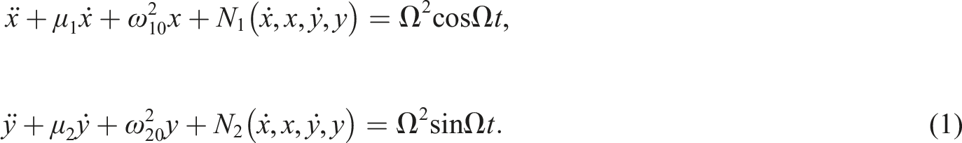
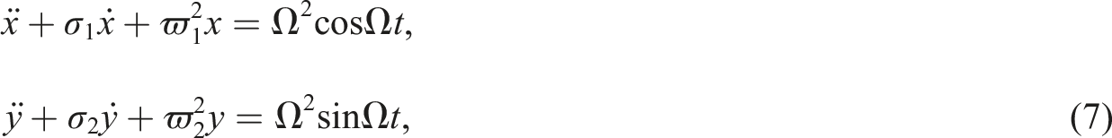
Modelling of the rotational motion of 6-DOF rigid body according to the Bobylev–Steklov is conditions demonstrated by He et al. Nonlinear vibration is an attendant phenomenon of rolling machinery. The rotor misalignments, the coupling imbalance, and the erode between the rotating parts and the stator are the main reasons for rotating machinery vibrations. We are interested in the dynamics of a forced system with two degrees of freedom of two damping linear oscillators with cubic stiffness nonlinearities. The oscillators are assumed to be coupled with conjugate cubic terms. Throughout this paper ${\mu }_1$ and ${\mu }_2$ as well as ${\omega }_{10\hspace{0.17em}}^2$ and ${\omega }_{20}^2$ are assumed to be nonnegative real numbers. A system of damped and forced Duffing oscillators is considered which satisfies the mixed value problem and has many engineering applications as mentioned in ³⁸ as follows

$\begin{array}{l}\ddot{x}+{\mu }_1\dot{x}+{\omega }_{10}^{2}x+N_1\left(\dot{x},x,\dot{y},y\right)={\mathrm{\Omega }}^2\cos \mathrm{\Omega }t,\\ \ddot{y}+{\mu }_2\dot{y}+{\omega }_{20}^{2}y+N_2\left(\dot{x},x,\dot{y},y\right)={\mathrm{\Omega }}^2\sin \mathrm{\Omega }t\end{array}.$

(1)

Here, the dynamic variables of the system, x(t) and y(t) stand for scaled displacements of the two oscillators, ${\mu }_1$ and ${\mu }_2$ play the roles of damping coefficients, ${\omega }_{10}^2$ and ${\omega }_{20}^2$ are two different squared linear natural frequencies, $\mathrm{\Omega }$ is the exciting frequency, and $N_1\left(\dot{x},x,\dot{y},y\right)$ and $N_2\left(\dot{x},x,\dot{y},y\right)$ represent two diffusive coupling functions between $x\left(t\right)$ and $y\left(t\right)$ whose derivatives of some coupled cubic nonlinear terms are given below

$\begin{array}{l}{N}_1\left(\dot{x},x,\dot{y},y\right)={\alpha }_1{x}^3+{\alpha }_2{x}^2\dot{x}+{\alpha }_{3}x{\dot{x}}^2+{\alpha }_{4}x{y}^2+{\alpha }_{5}xy\dot{y}+{\alpha }_{6}x{\dot{y}}^2+{\alpha }_7\dot{x}{y}^2+{\alpha }_{8}y\dot{x}\dot{y},\\ N_2\left(\dot{x},x,\dot{y},y\right)={\beta }_1{y}^3+{\beta }_2{y}^2\dot{y}+{\beta }_{3}y{\dot{y}}^2+{\beta }_{4}y{x}^2+{\beta }_{5}yx\dot{x}+{\beta }_{6}y{\dot{x}}^2+{\beta }_7\dot{y}{x}^2+{\beta }_{8}x\dot{x}\dot{y}.\end{array}$

(2)

This system is subject to the initial conditions defined as ³⁹

$\begin{array}{l}x\left(0\right)=A,\hspace{0.17em}\dot{x}\left(0\right)=0,\\ y\left(0\right)=B,\hspace{0.17em}\dot{y}\left(0\right)=0,\end{array}$

(3)

where $A$ and $B$ are the initial amplitudes of the oscillator.

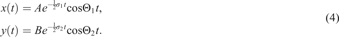
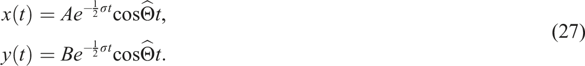
The main objective of this work revolves around obtaining a suitable solution to the case of the non-conservative system (1) in the simplest and least complicated way. The expected homogenous solution requires to be in the following form

$\begin{array}{l}x\left(t\right)=A{e}^{-\frac{1}{2}{\sigma }_{1}t}\cos {\mathrm{\Theta }}_{1}t,\\ y\left(t\right)=B{e}^{-\frac{1}{2}{\sigma }_{2}t}\cos {\mathrm{\Theta }}_{2}t.\end{array}$

(4)

where ${\sigma }_i>0$ represents all damping forces and ${\mathrm{\Theta }}_i$ denoted to the total frequencies. The above solutions are formulated through the exponential of the negative damping coefficients ${\sigma }_1$ and ${\sigma }_2$ that ensure the solution will avoid divergence and instability.

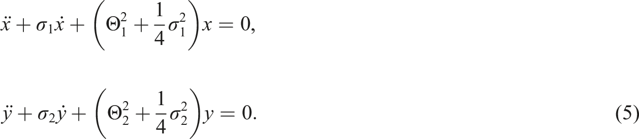
According to the hypothesis of the homogeneous solutions, as suggested by (4), whereas the homogenous differential equations of the system (1) must have the following linear forms

$\begin{array}{l}\ddot{x}+{\sigma }_1\dot{x}+\left({\mathrm{\Theta }}_1^2+\frac{1}{4}{\sigma }_1^2\right)x=0,\\ \ddot{y}+{\sigma }_2\dot{y}+\left({\mathrm{\Theta }}_2^2+\frac{1}{4}{\sigma }_2^2\right)y=0.\end{array}$

(5)

The disappearance of the exciting frequency $\mathrm{\Omega }$ from the system (1) becomes the autonomous case. The presence of an external force leads to the creation of a state of harmonic resonance case. The mathematical approach is based on how to obtain the nonlinear system predicted in (5).

The methodology

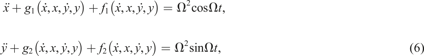
It can be regarded that the system is composed of four parts: two damping forces and two restoring forces, which can be rewritten in terms of these parts as follows

$\begin{array}{l}\ddot{x}+g_1\left(\dot{x},x,\dot{y},y\right)+f_1\left(\dot{x},x,\dot{y},y\right)={\mathrm{\Omega }}^2\cos \mathrm{\Omega }t,\\ \ddot{y}+g_2\left(\dot{x},x,\dot{y},y\right)+f_2\left(\dot{x},x,\dot{y},y\right)={\mathrm{\Omega }}^2\sin \mathrm{\Omega }t,\end{array}$

(6)

where the functions $g_1\left(\dot{x},x,\dot{y},y\right)$ and $g_2\left(\dot{x},x,\dot{y},y\right)$ are odd functions selected to have a common damping factor $\dot{x}$ and $\dot{y}$ , respectively. The chosen of $g_{\mathrm{1,2}}\left(\dot{x},x,\dot{y},y\right)$ will be the basis of the damping force in the linearized form. Similarly, the functions $f_1\left(\dot{x},x,\dot{y},y\right)$ and $f_2\left(\dot{x},x,\dot{y},y\right)$ are odd functions chosen to have the collective linear variables $x$ and $y$ , respectively. These functions are the essence of the nonlinear restoring forces and will generate the natural frequencies of the linearized system. Following El-Dib^34–36 the equivalent linear system is sought in the form

$\begin{array}{l}\ddot{x}+{\sigma }_1\dot{x}+{\varpi }_1^{2}x={\mathrm{\Omega }}^2\cos \mathrm{\Omega }t,\\ \ddot{y}+{\sigma }_2\dot{y}+{\varpi }_2^{2}y={\mathrm{\Omega }}^2\sin \mathrm{\Omega }t,\end{array}$

(7)

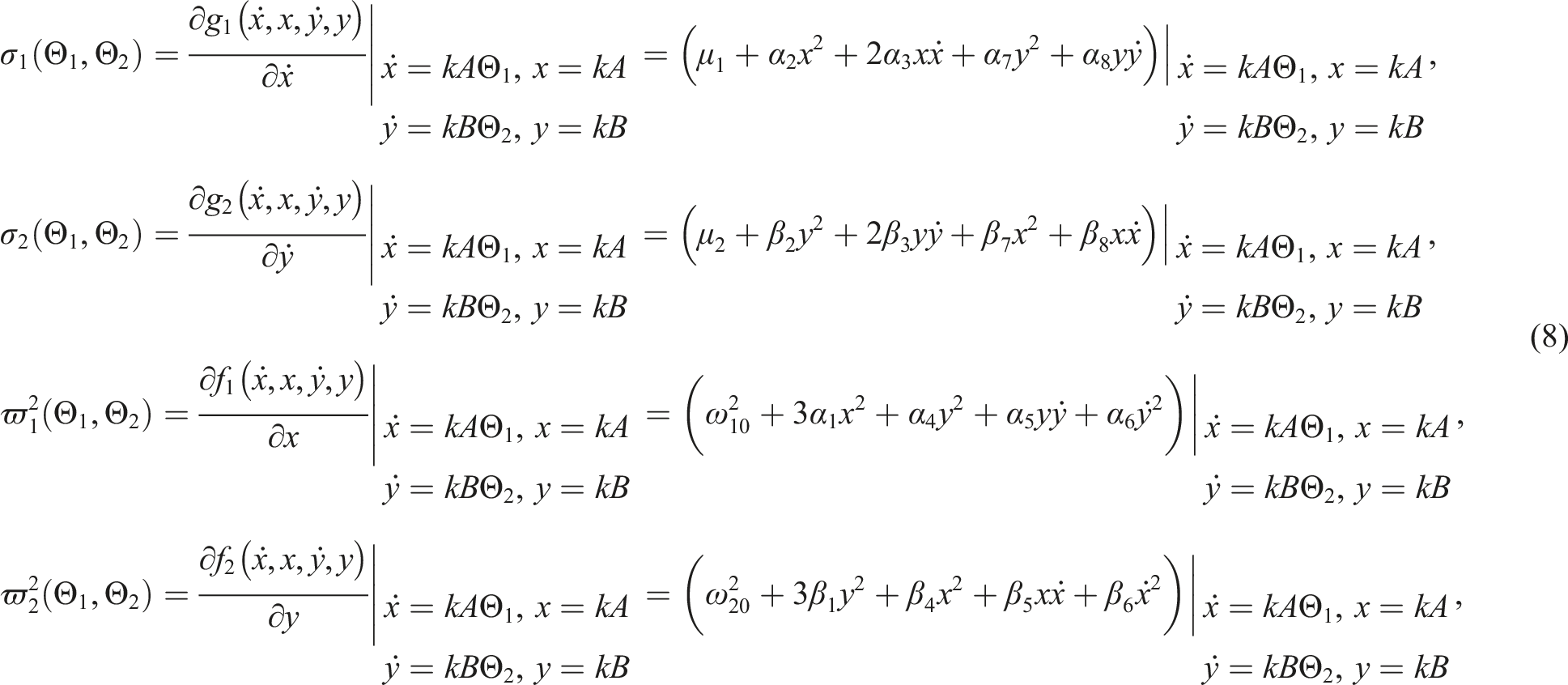
where ${\sigma }_1$ and ${\sigma }_2$ are the total damping coefficients. ${\varpi }_1^2$ and ${\varpi }_2^2$ indicate the natural frequencies of the linear system (7). These natural frequencies are readily obtained by a simplest method demonastrated by He.^23,24,29,30 However, the coefficients appearing in the above system should be estimated in terms of the total frequencies ${\mathrm{\Theta }}_1$ and ${\mathrm{\Theta }}_2$ . Follow El-Dib ³⁶ these coefficients are performed below

$\begin{array}{l}{\sigma }_1\left({\mathrm{\Theta }}_1,{\mathrm{\Theta }}_2\right)={\frac{\partial g_1\left(\dot{x},x,\dot{y},y\right)}{\partial \dot{x}}|}_{\begin{array}{l}\dot{x}=kA{\mathrm{\Theta }}_1,\hspace{0.17em}x=kA\\ \dot{y}=kB{\mathrm{\Theta }}_2,\hspace{0.17em}y=kB\end{array}}={\left({\mu }_1+{\alpha }_2{x}^2+2{\alpha }_{3}x\dot{x}+{\alpha }_7{y}^2+{\alpha }_{8}y\dot{y}\right)|}_{\begin{array}{l}\dot{x}=kA{\mathrm{\Theta }}_1,\hspace{0.17em}x=kA\\ \dot{y}=kB{\mathrm{\Theta }}_2,\hspace{0.17em}y=kB\end{array}},\\ {\sigma }_2\left({\mathrm{\Theta }}_1,{\mathrm{\Theta }}_2\right)={\frac{\partial g_2\left(\dot{x},x,\dot{y},y\right)}{\partial \dot{y}}|}_{\begin{array}{l}\dot{x}=kA{\mathrm{\Theta }}_1,\hspace{0.17em}x=kA\\ \dot{y}=kB{\mathrm{\Theta }}_2,\hspace{0.17em}y=kB\end{array}}={\left({\mu }_2+{\beta }_2{y}^2+2{\beta }_{3}y\dot{y}+{\beta }_7{x}^2+{\beta }_{8}x\dot{x}\right)|}_{\begin{array}{l}\dot{x}=kA{\mathrm{\Theta }}_1,\hspace{0.17em}x=kA\\ \dot{y}=kB{\mathrm{\Theta }}_2,\hspace{0.17em}y=kB\end{array}},\hspace{0.17em}\\ {\varpi }_1^2\left({\mathrm{\Theta }}_1,{\mathrm{\Theta }}_2\right)={\frac{\partial f_1\left(\dot{x},x,\dot{y},y\right)}{\partial x}|}_{\begin{array}{l}\dot{x}=kA{\mathrm{\Theta }}_1,\hspace{0.17em}x=kA\\ \dot{y}=kB{\mathrm{\Theta }}_2,\hspace{0.17em}y=kB\end{array}}={\left({\omega }_{10}^2+3{\alpha }_1{x}^2+{\alpha }_4{y}^2+{\alpha }_{5}y\dot{y}+{\alpha }_6{\dot{y}}^2\right)|}_{\begin{array}{l}\dot{x}=kA{\mathrm{\Theta }}_1,\hspace{0.17em}x=kA\\ \dot{y}=kB{\mathrm{\Theta }}_2,\hspace{0.17em}y=kB\end{array}},\hspace{0.17em}\\ {\varpi }_2^2\left({\mathrm{\Theta }}_1,{\mathrm{\Theta }}_2\right)={\frac{\partial f_2\left(\dot{x},x,\dot{y},y\right)}{\partial y}|}_{\begin{array}{l}\dot{x}=kA{\mathrm{\Theta }}_1,\hspace{0.17em}x=kA\\ \dot{y}=kB{\mathrm{\Theta }}_2,\hspace{0.17em}y=kB\end{array}}={\left({\omega }_{20}^2+3{\beta }_1{y}^2+{\beta }_4{x}^2+{\beta }_{5}x\dot{x}+{\beta }_6{\dot{x}}^2\right)|}_{\begin{array}{l}\dot{x}=kA{\mathrm{\Theta }}_1,\hspace{0.17em}x=kA\\ \dot{y}=kB{\mathrm{\Theta }}_2,\hspace{0.17em}y=kB\end{array}},\end{array}$

(8)

where the located displacements are assumed to be $x=kA,$ and $y=kB.$ On the other side, the located velocities are estimated as $\dot{x}=kA{\mathrm{\Theta }}_1,\hspace{0.17em}\dot{y}=kB{\mathrm{\Theta }}_2.$ The parameter $k$ is defined as $k=\frac{1}{2\sqrt{n-r}},$ where $n$ indicates the total order of the system and $r$ refers to the freedom degree in the system. Employing $n=4$ and $r=2$ ; therefore, the desired value $k$ is found to be

$k=\frac{1}{2\sqrt{2}}.$

(9)

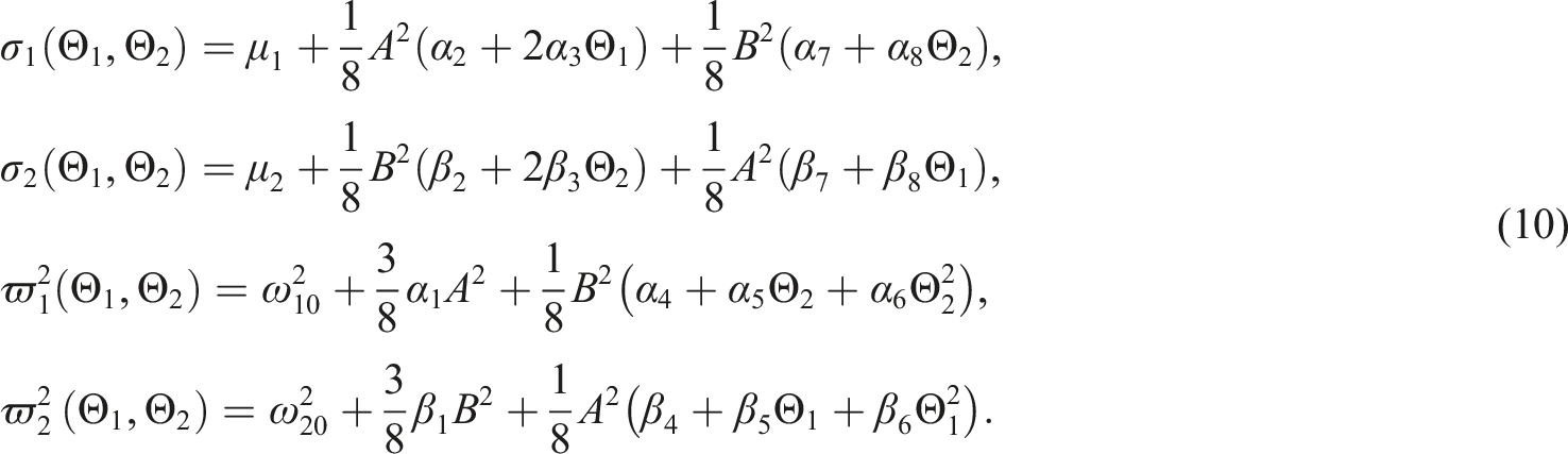
Consequently, the coefficients that appear in the system (7) have the following values

$\begin{array}{l}{\sigma }_1\left({\mathrm{\Theta }}_1,{\mathrm{\Theta }}_2\right)={\mu }_1+\frac{1}{8}{A}^2\left({\alpha }_2+2{\alpha }_3{\mathrm{\Theta }}_1\right)+\frac{1}{8}{B}^2\left({\alpha }_7+{\alpha }_8{\mathrm{\Theta }}_2\right),\\ {\sigma }_2\left({\mathrm{\Theta }}_1,{\mathrm{\Theta }}_2\right)={\mu }_2+\frac{1}{8}{B}^2\left({\beta }_2+2{\beta }_3{\mathrm{\Theta }}_2\right)+\frac{1}{8}{A}^2\left({\beta }_7+{\beta }_8{\mathrm{\Theta }}_1\right),\\ {\varpi }_1^2\left({\mathrm{\Theta }}_1,{\mathrm{\Theta }}_2\right)={\omega }_{10}^2+\frac{3}{8}{\alpha }_1{A}^2+\frac{1}{8}{B}^2\left({\alpha }_4+{\alpha }_5{\mathrm{\Theta }}_2+{\alpha }_6{\mathrm{\Theta }}_2^2\right),\\ {\varpi }_2^2\hspace{0.17em}\left({\mathrm{\Theta }}_1,{\mathrm{\Theta }}_2\right)={\omega }_{20}^2+\frac{3}{8}{\beta }_1{B}^2+\frac{1}{8}{A}^2\left({\beta }_4+{\beta }_5{\mathrm{\Theta }}_1+{\beta }_6{\mathrm{\Theta }}_1^2\right).\end{array}$

(10)

To this end, system (7) represents approximately a simple mathematical model for the coupled nonlinear damping oscillators that are considered in the system (1). The simplicity that system (6) displays lies in the fact that each equation is separately solvable. There appears to be a separation between its variables, but the duplication lies within the coefficients. The coupling is inherent in the formation of the coefficients as seen in the definitions (10). According to this structure, the solutions of the system (6) are easy to establish.

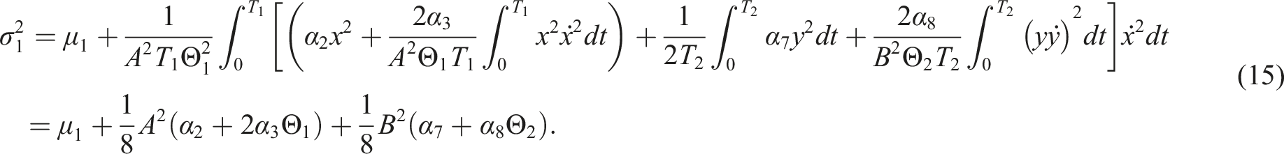
It is noted that the results obtained in (10) can be derived by applying the weighted residuals property^40,41 to estimate the frequencies ${\varpi }_1^2\left({\mathrm{\Theta }}_1,{\mathrm{\Theta }}_2\right)$ and ${\varpi }_2^2\hspace{0.17em}\left({\mathrm{\Theta }}_1,{\mathrm{\Theta }}_2\right)$ and to ensure that the parameter $k$ given by (9) is the suitable value to estimate the frequency through the derivative approach. The weighted residuals property can be applied twice to the two functions $f_1\left(\dot{x},x,\dot{y},y\right)$ and $f_2\left(\dot{x},x,\dot{y},y\right)$ since they are composed of coupled forces. Therefore, the first step on the function $f_1\left(\dot{x},x,\dot{y},y\right)$ is to evaluate the residual corresponding to the non-main variable given in equation (6) while the weighted residual is applied to the main variable as shown below:

Suppose the trial solutions of the un-forced case are given by $x\left(t\right)=A\cos \hspace{0.17em}{\mathrm{\Theta }}_{1}t\hspace{0.17em}$ and $y\left(t\right)=B\cos \hspace{0.17em}{\mathrm{\Theta }}_{2}t\hspace{0.17em},$ then the first step is given by

$R_{10}\left(t\right)={\alpha }_1{x}^3+\frac{x}{2T_2}{\int }_0^{T_2}\left({\alpha }_4{y}^2+{\alpha }_6{\dot{y}}^2\right)dt+\frac{2x{\alpha }_5}{B^2{\mathrm{\Theta }}_2{T}_2}{\int }_0^{T_2}{y}^2{\dot{y}}^{2}dt;\hspace{0.17em}{T}_2=\frac{\pi }{2{\mathrm{\Theta }}_2}.$

(11)

Similar, it can be written

$R_{20}\left(t\right)={\beta }_1{y}^3+\frac{y}{2T_1}{\int }_0^{T_1}\left({\beta }_4{x}^2+{\beta }_6{\dot{x}}^2\right)dt+\frac{2y{\beta }_5}{A^2{\mathrm{\Theta }}_1{T}_1}{\int }_0^{T_1}{x}^2{\dot{x}}^{2}dt;\hspace{0.17em}{T}_1=\frac{\pi }{2{\mathrm{\Theta }}_1}.$

(12)

The second step is the estimated of the frequencies of the nonlinear restoring forces ${\varpi }_1^2$ and ${\varpi }_2^2$ as given below

${\varpi }_1^2\left({\mathrm{\Theta }}_1,{\mathrm{\Theta }}_2\right)={\omega }_{10}^2+\frac{1}{A{T}_1}{\int }_0^{T_1}{R}_{10}\left(t\right)x\left(t\right)dt={\omega }_{10}^2+\frac{3}{8}{A}^2{\alpha }_1+\frac{1}{8}{B}^2\left({\alpha }_4+{\alpha }_5{\mathrm{\Theta }}_2+{\alpha }_6{\mathrm{\Theta }}_2^2\right),$

(13)

${\varpi }_2^2\left({\mathrm{\Theta }}_1,{\mathrm{\Theta }}_2\right)={\omega }_{20}^2+\frac{1}{B{T}_2}{\int }_0^{T_2}{R}_{20}\left(t\right)y\left(t\right)dt={\omega }_{20}^2+\frac{3}{8}{B}^2{\beta }_1+\frac{1}{8}{A}^2\left({\beta }_4+{\beta }_5{\mathrm{\Theta }}_1+{\beta }_6{\mathrm{\Theta }}_1^2\right).$

(14)

Also, it is found that the damping coefficients ${\sigma }_1^2$ a ${\sigma }_2^2$ re estimated on the same two steps of the integration as follows

$\begin{array}{l}{\sigma }_1^2={\mu }_1+\frac{1}{A^2{T}_1{\mathrm{\Theta }}_1^2}{\int }_0^{T_1}\left[\left({\alpha }_2{x}^2+\frac{2{\alpha }_3}{A^2{\mathrm{\Theta }}_1{T}_1}{\int }_0^{T_1}{x}^2{\dot{x}}^{2}dt\right)+\frac{1}{2T_2}{\int }_0^{T_2}{\alpha }_7{y}^{2}dt+\frac{2{\alpha }_8}{B^2{\mathrm{\Theta }}_2{T}_2}{\int }_0^{T_2}{\left(y\dot{y}\right)}^{2}dt\right]{\dot{x}}^{2}dt\\ ={\mu }_1+\frac{1}{8}{A}^2\left({\alpha }_2+2{\alpha }_3{\mathrm{\Theta }}_1\right)+\frac{1}{8}{B}^2\left({\alpha }_7+{\alpha }_8{\mathrm{\Theta }}_2\right).\end{array}$

(15)

$\begin{array}{l}{\sigma }_2^2={\mu }_2+\frac{1}{B^2{T}_2{\mathrm{\Theta }}_2^2}{\int }_0^{T_2}\left[\left({\beta }_2{y}^2+\frac{2{\beta }_3}{B^2{\mathrm{\Theta }}_2{T}_2}{\int }_0^{T2}{y}^2{\dot{y}}^{2}dt\right)+\frac{1}{2T_1}{\int }_0^{T_1}{\beta }_7{x}^{2}dt+\frac{2{\beta }_8}{A^2{\mathrm{\Theta }}_1{T}_1}{\int }_0^{T1}{\left(x\dot{x}\right)}^{2}dt\right]{\dot{y}}^{2}dt\\ ={\mu }_2+\frac{1}{8}{B}^2\left({\beta }_2+2{\beta }_3{\mathrm{\Theta }}_2\right)+\frac{1}{8}{A}^2\left({\beta }_7+{\beta }_8{\mathrm{\Theta }}_1\right).\end{array}$

(16)

It is observed that the results obtained by the differential forms assuming $k=\frac{1}{2\sqrt{2}}$ have coincided with the results derived through the integral forms.

Behavior of the unforced system

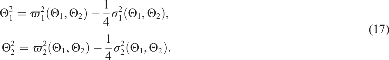
The autonomous case is the unforced system. This initial investigation analyzes the behavior of (7) for the case of $\mathrm{\Omega }\to 0$ . Therefore, the governing equations of the unforced case yield the solutions (4), where the total frequencies for the non-conservative system are defined as

$\begin{array}{l}{\mathrm{\Theta }}_1^2={\varpi }_1^2\left({\mathrm{\Theta }}_1,{\mathrm{\Theta }}_2\right)-\frac{1}{4}{\sigma }_1^2\left({\mathrm{\Theta }}_1,{\mathrm{\Theta }}_2\right),\\ \hspace{0.17em}{\mathrm{\Theta }}_2^2={\varpi }_2^2\left({\mathrm{\Theta }}_1,{\mathrm{\Theta }}_2\right)-\frac{1}{4}{\sigma }_2^2\left({\mathrm{\Theta }}_1,{\mathrm{\Theta }}_2\right).\end{array}$

(17)

The definitions given in the system (17) are two complicated coupled relations in the two non-conservative frequencies ${\mathrm{\Theta }}_1$ and ${\mathrm{\Theta }}_2$ . The linear natural frequencies ${\omega }_{10}^2$ and ${\omega }_{20}^2$ are included in the nonlinear natural frequencies ${\varpi }_1^2$ and ${\varpi }_2^2$ . Further, the last two frequencies are functions in the total frequencies ${\mathrm{\Theta }}_1$ and ${\mathrm{\Theta }}_2$ . If there is some relation between the two linear frequencies, it is known as the internal resonance case. On the other side, if a relation between ${\mathrm{\Theta }}_1$ and ${\mathrm{\Theta }}_2$ is found, then it is called the nonlinear resonance case.

The non-internal and without the nonlinear resonance case

The non-internal resonance is desired when there is no relationship between the two original natural frequencies ${\omega }_{10}^2$ and ${\omega }_{20}^2$ . When there is no relationship between the frequencies ${\mathrm{\Theta }}_1$ and ${\mathrm{\Theta }}_2$ , it is called a non-resonance case. ⁴¹

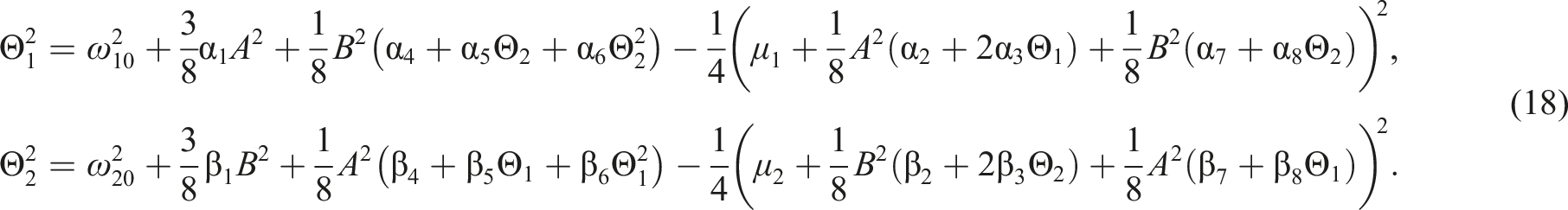
To study the behavior of the solution in the non-internal and free of the nonlinear resonance cases, (10) is inserted into (17) to give

$\begin{array}{l}{\mathrm{\Theta }}_1^2={\omega }_{10}^2+\frac{3}{8}{\alpha }_1{A}^2+\frac{1}{8}{B}^2\left({\alpha }_4+{\alpha }_5{\mathrm{\Theta }}_2+{\alpha }_6{\mathrm{\Theta }}_2^2\right)-\frac{1}{4}{\left({\mu }_1+\frac{1}{8}{A}^2\left({\alpha }_2+2{\alpha }_3{\mathrm{\Theta }}_1\right)+\frac{1}{8}{B}^2\left({\alpha }_7+{\alpha }_8{\mathrm{\Theta }}_2\right)\right)}^2,\\ {\mathrm{\Theta }}_2^2={\omega }_{20}^2+\frac{3}{8}{\beta }_1{B}^2+\frac{1}{8}{A}^2\left({\beta }_4+{\beta }_5{\mathrm{\Theta }}_1+{\beta }_6{\mathrm{\Theta }}_1^2\right)-\frac{1}{4}{\left({\mu }_2+\frac{1}{8}{B}^2\left({\beta }_2+2{\beta }_3{\mathrm{\Theta }}_2\right)+\frac{1}{8}{A}^2\left({\beta }_7+{\beta }_8{\mathrm{\Theta }}_1\right)\right)}^2.\end{array}$

(18)

These are two rigorous coupled equations in the two non-conservative frequencies ${\mathrm{\Theta }}_1$ and ${\mathrm{\Theta }}_2$ . This system contains coupled polynomials of the second degree in ${\mathrm{\Theta }}_1$ and ${\mathrm{\Theta }}_2$ . The application of the algebraic process to separation should lead to two separated polynomials of the fourth degree

$\begin{array}{l}{a}_4{\mathrm{\Theta }}_1^4+a_3{\mathrm{\Theta }}_1^3+a_2{\mathrm{\Theta }}_1^2+a_1{\mathrm{\Theta }}_1+a_0=0,\\ b_4{\mathrm{\Theta }}_2^4+b_3{\mathrm{\Theta }}_2^3+b_2{\mathrm{\Theta }}_2^2+b_1{\mathrm{\Theta }}_2+b_0=0.\end{array}$

(19)

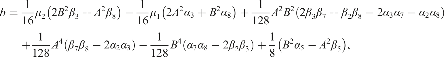
The coefficients $a_j$ and $b_j;\hspace{0.17em}j=0:4$ are straightforward and lengthy. To limit the length of the paper, they will be omitted.

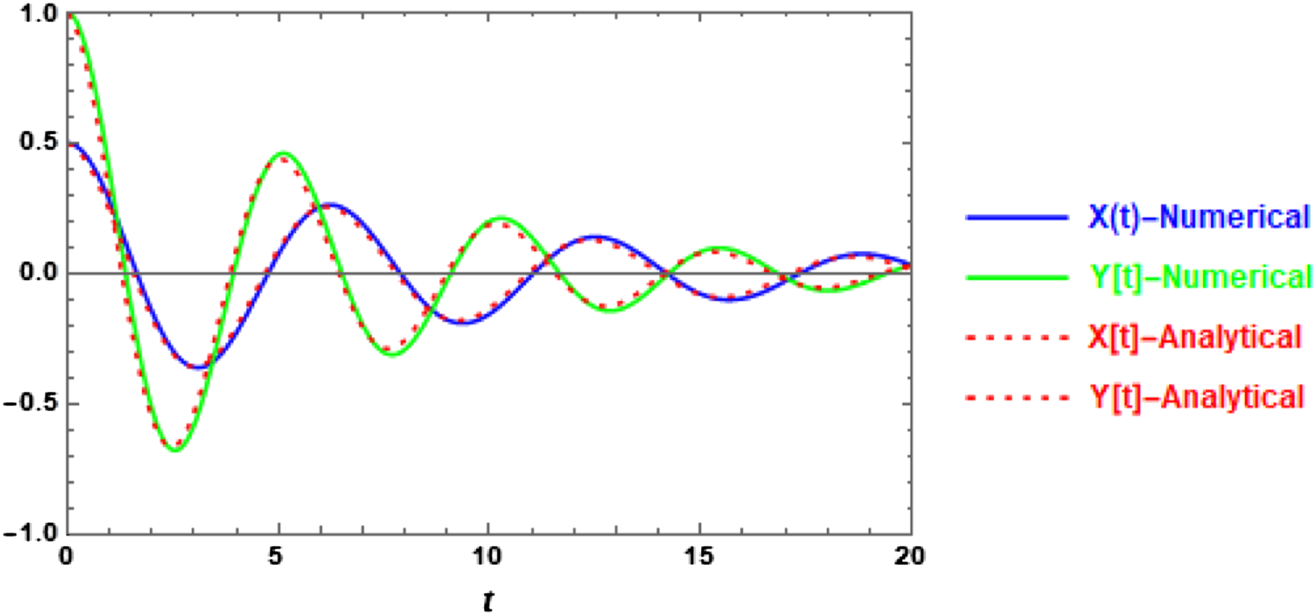
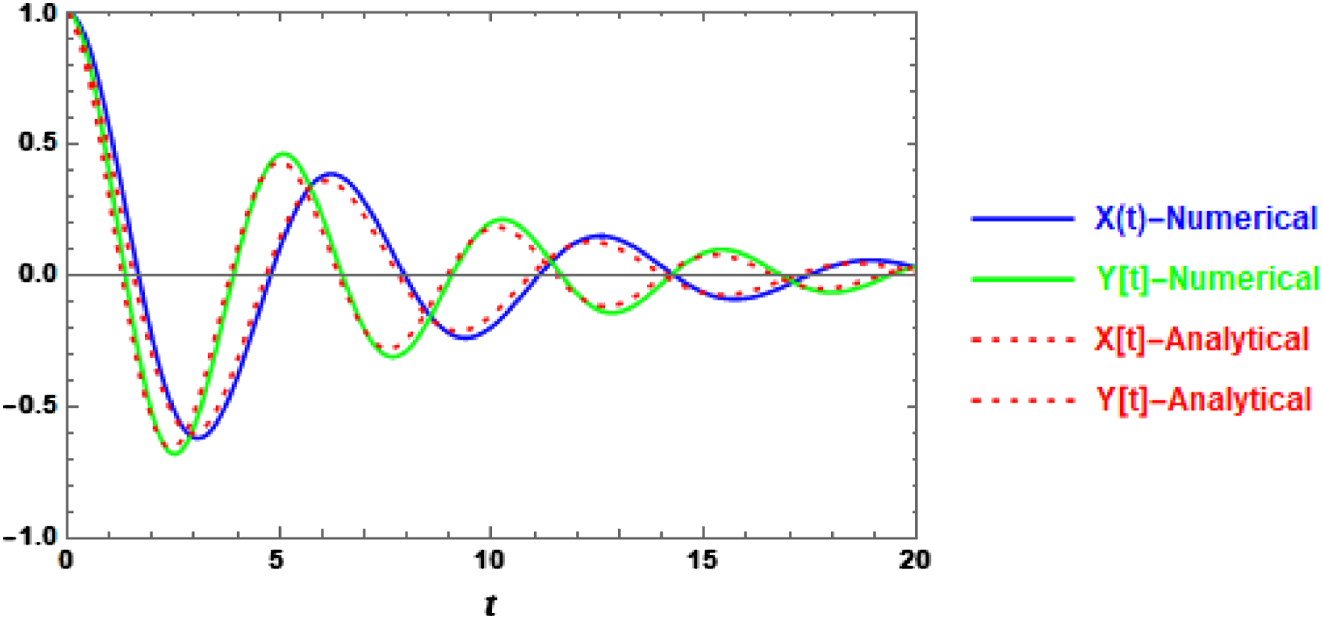
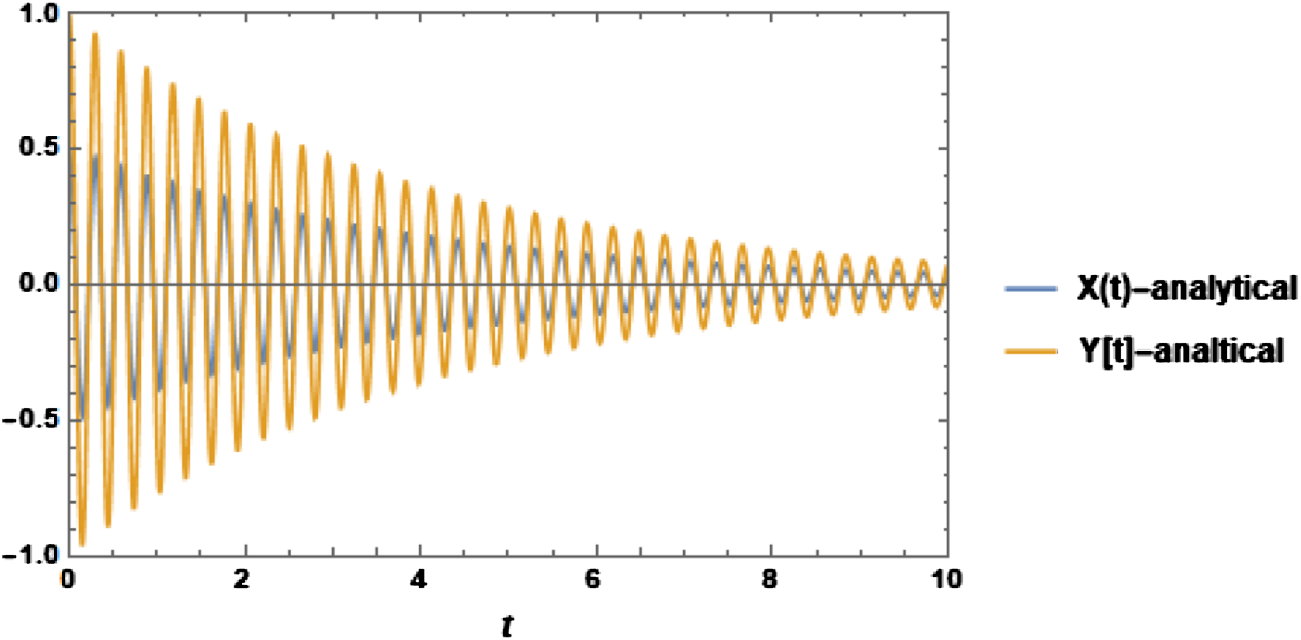
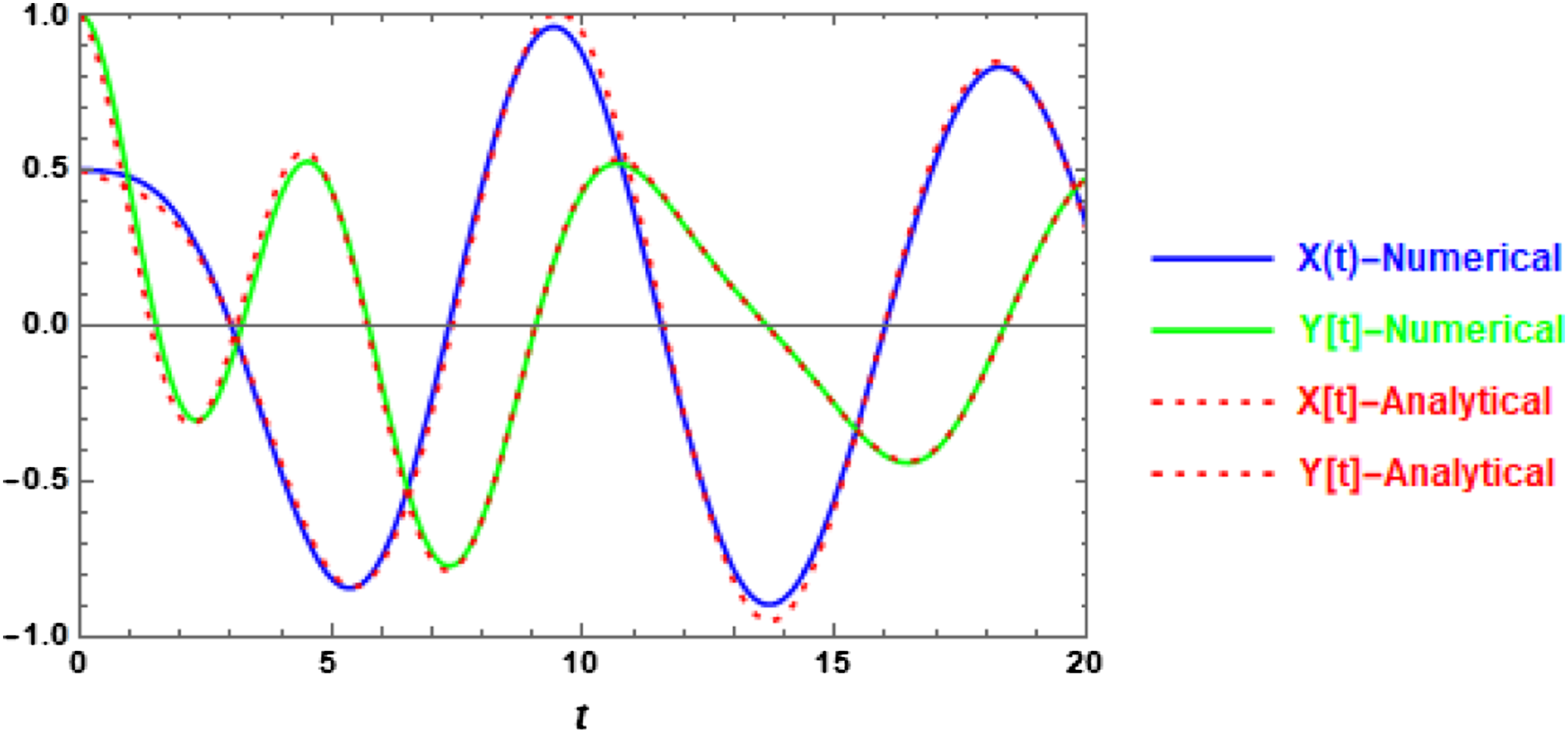
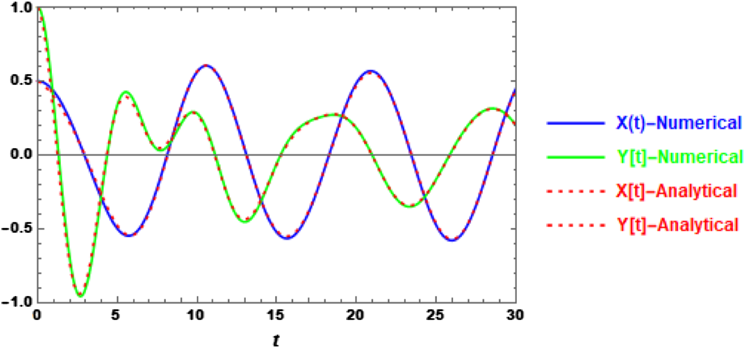
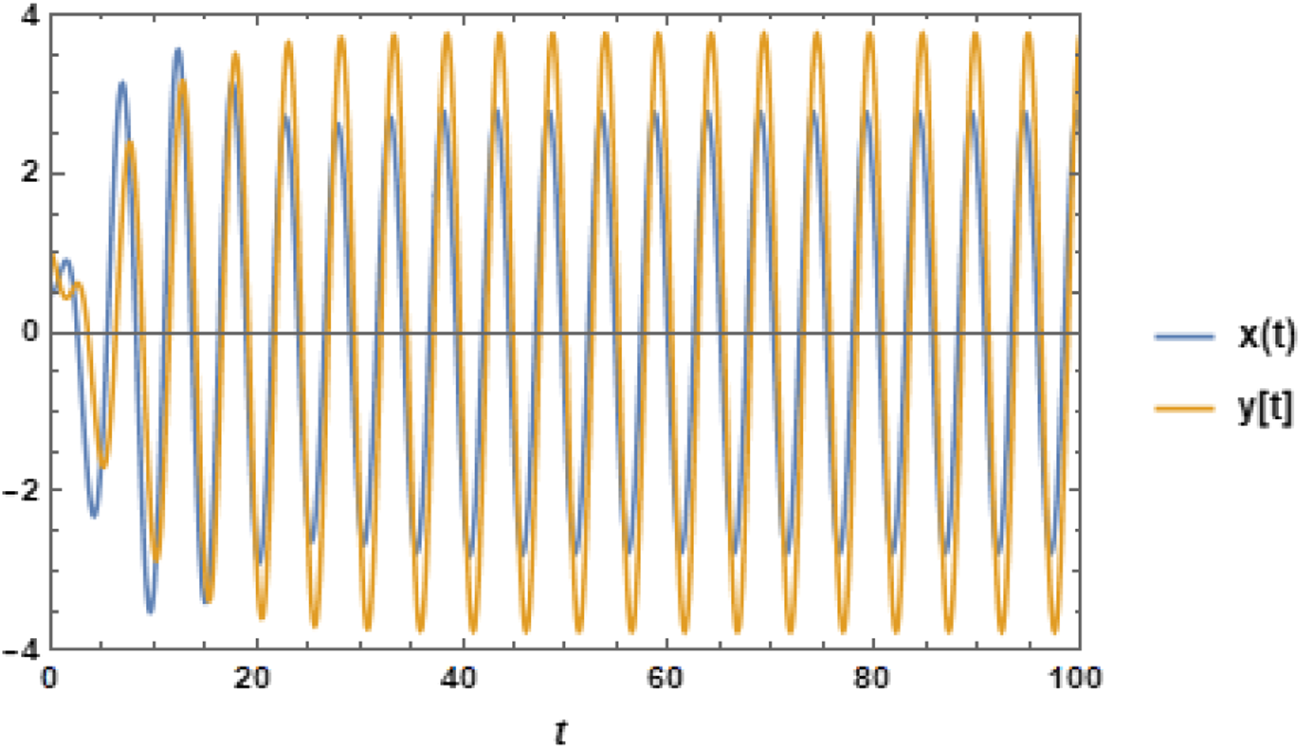
To ensure the effectiveness of the current technique, the results of the bounded solution given the system (4) are compared with the numerical solution of the considered unforced system (1). The analytical solution (4) mainly depends on the values of the frequencies (19). Therefore, Figure 1 is designed to demonstrate the analytical bounded solution together with the numerical solution given by the program built-in Mathematica. The calculations are made for a system having the particulars ${\mu }_1=0.2,\hspace{0.17em}{\mu }_2=0.3,\hspace{0.17em}{\omega }_{10}^2=1,\hspace{0.17em}{\omega }_{20}^2=1.5,$ and all the nonlinear coefficients take the same value of $0.05$ . The initial oscillation amplitudes are chosen to be $A=0.5$ and $B=1$ . Through this calculation, the use of the chosen system reveals that the approximate values of the frequencies are ${\mathrm{\Theta }}_1=1.00797$ and ${\mathrm{\Theta }}_2=1.22357.$ Also, the decaying parameters ${\sigma }_1=0.21861$ and ${\sigma }_2=0.324682$ . As shown from this figure, the amplitudes of the solutions $x\left(t\right)$ and $y\left(t\right)$ start from two different points. Over time, each wave-time solution is exhibited alone. It is shown that the amplitude of each wave gradually decreases until it decays. The validation of the accuracy through the numerical solution showed an excellent agreement between the two methodologies.

Figure 1.

The comparison between the numerical solution of the unforced system (1) and its analytical solution given in the system (4).

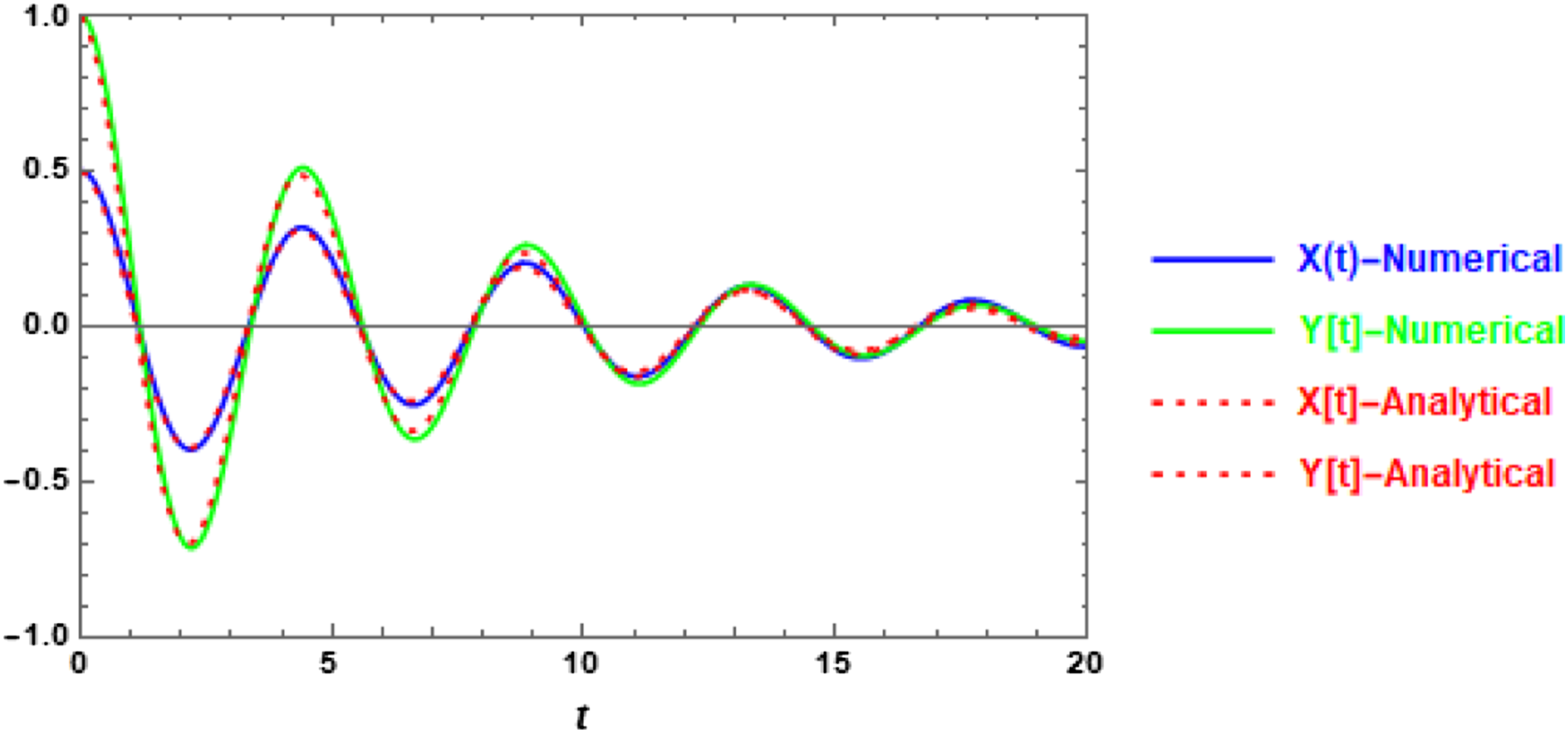
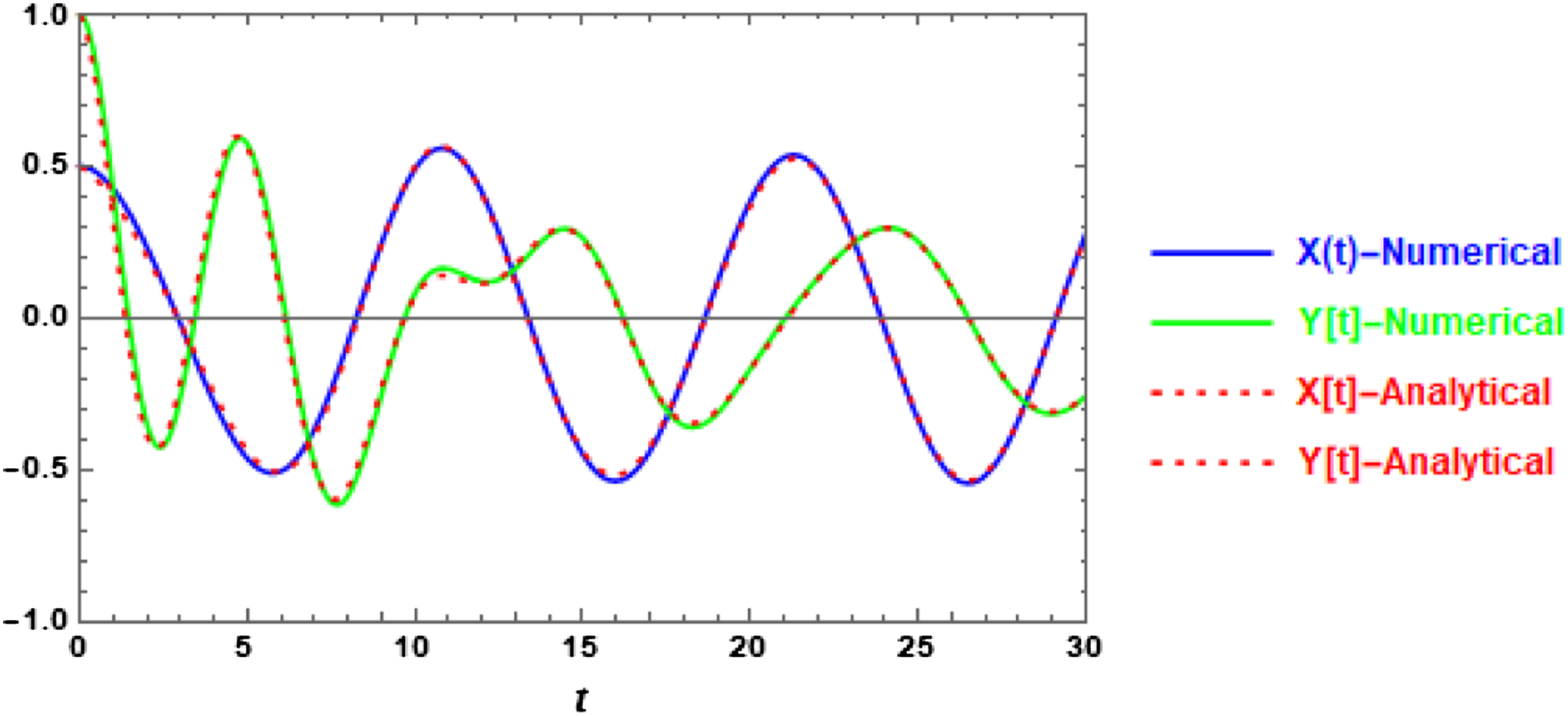
Figure 2 is designed for the exact internal resonance case, in which the initial amplitudes $A$ and $B$ are chosen to be the same $A=B=1$ , and the linear damping coefficient ${\mu }_1$ is taken to be the same ${\mu }_2$ ( ${\mu }_1={\mu }_2=0.3$ ). As shown from this figure, the amplitudes of the solutions $x\left(t\right)$ and $y\left(t\right)$ start from the same point, from which the natural frequencies are randomly distributed. It is observed that the two wave-time solutions $x\left(t\right)$ and $y\left(t\right)$ are exhibited alone as shown in Figure 1.

Figure 2.

The comparison between the numerical solution of the unforced system (1) and its analytical solution given in the system (4). The calculations are made for the same system given in Figure 1 except that $A=B=1$ and ${\mu }_1={\mu }_2=0.3$ .

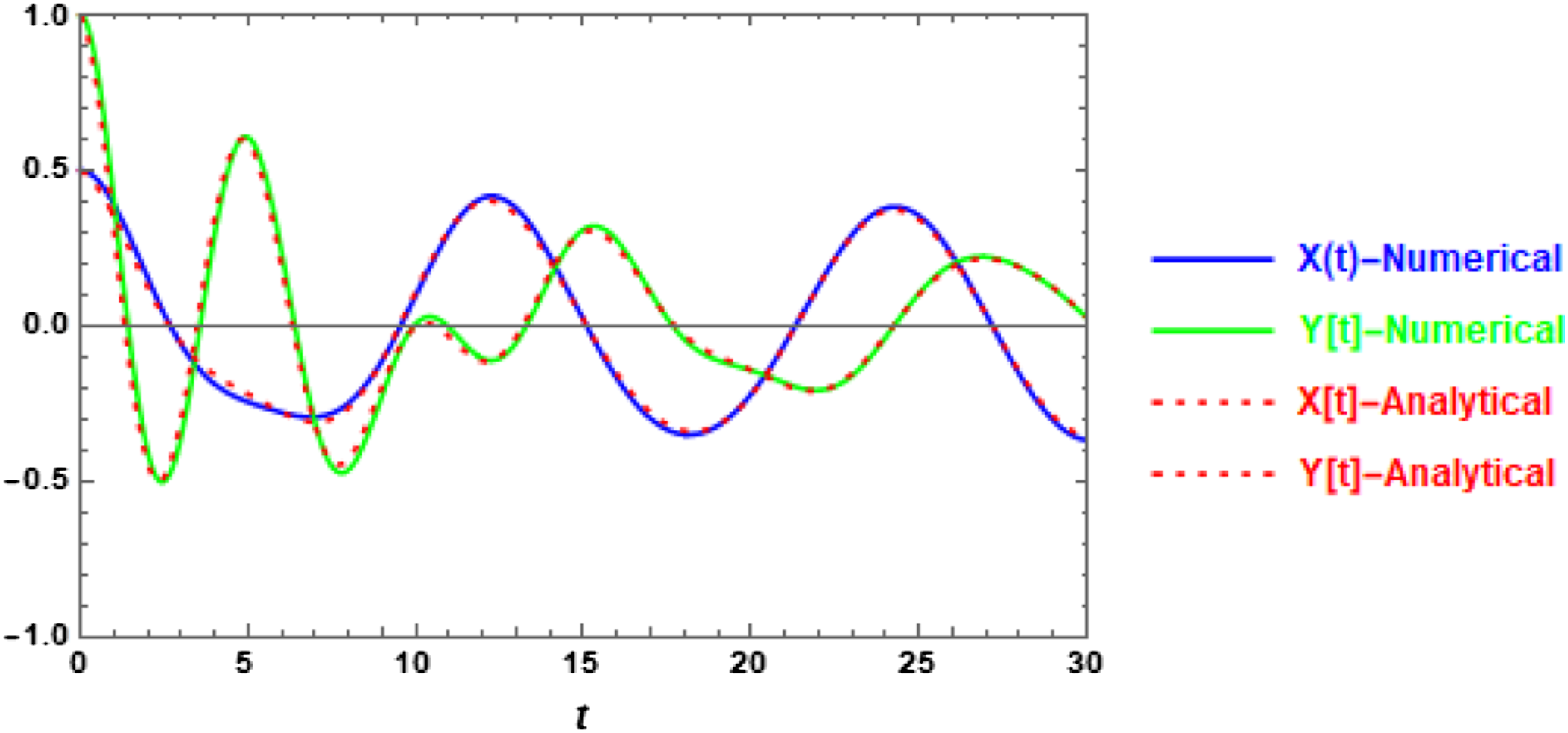
The examination of equal linear frequency ${\omega }_{10}^2={\omega }_{20}^2=2$ has been graphed as displayed in Figure 3. The calculations are made to the same system as given in Figure 1. This case is known as the sharp internal resonance case where ${\omega }_{10}^2$ is exactly equal to ${\omega }_{20}^2$ , and accordingly ${\mathrm{\Theta }}_1=1.42128\hspace{0.17em}\&\hspace{0.17em}{\mathrm{\Theta }}_2=1.4138$ and ${\sigma }_1=0.22109\hspace{0.17em}\&\hspace{0.17em}{\sigma }_2=0.327706$ . It is observed that the two wave solutions $x\left(t\right)$ and $y\left(t\right)$ firstly behave like standing waves to the extent that their amplitudes gradually decrease and decay together at the same time. Over time, the two waves behave in the same attitude.

Figure 3.

Perturbation solutions with the corresponding numerical solution of the unforced system (1) in the case of the sharp internal resonance case for the same system considered in Figure 1 except that ${\omega }_{10}^2={\omega }_{20}^2=2$ , with different amplitudes and different linear damping coefficients.

The nonlinear resonance case

The nonlinear resonance case is desired when there is a relationship between the two frequencies ${\mathrm{\Theta }}_1$ and ${\mathrm{\Theta }}_2$ . It can be observed that the graph displayed in Figure 3 has been established in case there is no relation between the two frequencies ${\mathrm{\Theta }}_1$ and ${\mathrm{\Theta }}_2$ .

Analytically, the behavior of the solutions in the case of the nonlinear resonance case can be studied by employing ${\mathrm{\Theta }}_1\cong {\mathrm{\Theta }}_2=\mathrm{\Theta }$ into the system (4). Consequently, the two definitions of (19) give the following frequency relationship

${\varpi }_2^2\left(\mathrm{\Theta }\right)\cong {\varpi }_1^2\left(\mathrm{\Theta }\right)+\frac{1}{4}\left({\sigma }_2^2\left(\mathrm{\Theta }\right)-{\sigma }_1^2\left(\mathrm{\Theta }\right)\right)$

(20)

To estimate the total frequency satisfied in the nonlinear resonance case, insert the limiting of (8) where ${\mathrm{\Theta }}_1={\mathrm{\Theta }}_2\to \mathrm{\Theta }$ may be inserted into (18) to yield

$a{\mathrm{\Theta }}^2+b\mathrm{\Theta }+c=0,$

(21)

where the coefficients $a,\hspace{0.17em}b\&\hspace{0.17em}c$ are listed below

$a=\frac{1}{64}{\left(B^2{\beta }_3+\frac{1}{2}{A}^2{\beta }_8\right)}^2-\frac{1}{64}{\left(A^2{\alpha }_3+\frac{1}{2}{B}^2{\alpha }_8\right)}^2+\frac{1}{8}\left(B^2{\alpha }_6-A^2{\beta }_6\right),$

$\begin{array}{l}b=\frac{1}{16}{\mu }_2\left(2B^2{\beta }_3+A^2{\beta }_8\right)-\frac{1}{16}{\mu }_1\left(2A^2{\alpha }_3+B^2{\alpha }_8\right)+\frac{1}{128}{A}^2{B}^2\left(2{\beta }_3{\beta }_7+{\beta }_2{\beta }_8-2{\alpha }_3{\alpha }_7-{\alpha }_2{\alpha }_8\right)\\ +\frac{1}{128}{A}^4\left({\beta }_7{\beta }_8-2{\alpha }_2{\alpha }_3\right)-\frac{1}{128}{B}^4\left({\alpha }_7{\alpha }_8-2{\beta }_2{\beta }_3\right)+\frac{1}{8}\left(B^2{\alpha }_5-A^2{\beta }_5\right),\end{array}$

$c={\omega }_{10}^2-{\omega }_{20}^2+\frac{1}{8}{A}^2\left(3{\alpha }_1-{\beta }_4\right)-\frac{1}{8}{B}^2\left(3{\beta }_1-{\alpha }_4\right)+\frac{1}{4}{\left({\mu }_2+\frac{1}{8}{A}^2{\beta }_7+\frac{1}{8}{B}^2{\beta }_2\right)}^2-\frac{1}{4}{\left({\mu }_1+\frac{1}{8}{B}^2{\alpha }_7+\frac{1}{8}{A}^2{\alpha }_2\right)}^2.$

To discuss the stability behavior in the present resonance case, there is an essential condition that must be satisfied

$b^2-4ac>0.$

(22)

Provided that the two exponentials ${\sigma }_1$ and ${\sigma }_2$ are positive.

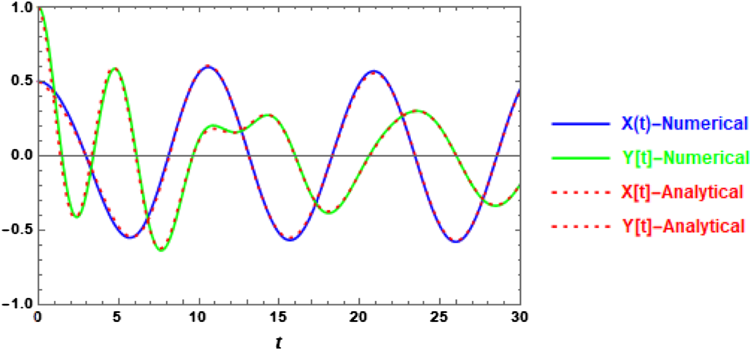
For more clarity, a drawing of the reached analytical solution is made. Employing the condition ${\mathrm{\Theta }}_1={\mathrm{\Theta }}_2$ , for the nonlinear resonance case, into the solution addressed by the system (4). Thus, it is appropriate to use the total frequency defined in (21) in the numerical calculation displayed in Figure 4. This figure illustrates the behavior of the solutions $x\left(t\right)$ and $y\left(t\right)$ in the nonlinear resonance case where the numerical calculation is made to the numerical parameters given in Figure 1, except that frequency-amplitudes relationship (21) is used in the present calculations. The investigation of Figure 4 shows that there is a standing wave behavior where the high of the wave solution $y\left(t\right)$ is larger than the height of the wave solution $x\left(t\right).$ s this calculation, the common total frequency is found to be $\mathrm{\Theta }=-10.9038$ and the total damping coefficients are ${\sigma }_1=0.10559$ and ${\sigma }_2=0.154478.$ It is noted that the linear frequencies ${\omega }_{10}^2\&{\omega }_{20}^2$ have been kept different in this calculation. Inspection of Figure 4 shows that at the sharp nonlinear resonance case, the two wave solutions $x\left(t\right)$ and $y\left(t\right)$ behave like standing waves with the same wavelength. The wavelength is constant over time. The major observation is a gradual decrease in the amplitudes. The amplitude of the $y\left(t\right)-$ solution decreases more rapidly than that of the $x\left(t\right)-$ solution until it decays with the same amplitude. In the sharp nonlinear resonance case, it is noted that there exists a small wavelength compared with the non-resonance case. It is generally observed that the amplitude of a vibrating body will decay exponentially untile until it rests.

Figure 4.

The behavior of the two wave solutions of (4) in the nonlinear resonance case of ${\mathrm{\Theta }}_1={\mathrm{\Theta }}_2$ , for the same system given in Figure 1 except that the total frequency (21) is used.

The internal resonance case

The present section is an attempt to generate the so-called internal resonance case from the nonlinear resonance case. It is known that an internal resonance case occurs when there is approaching of ${\omega }_{20}$ to ${\omega }_{10}$ This nearness is expressed by introducing a detuning parameter $\delta$ defined as follows

${\omega }_{20}^2={\omega }_{10}^2+\delta ,$

(23)

where the unknown $\delta$ needs to be determined. This can be accomplished below:

Following the structure of the approaching of the natural frequencies ${\varpi }_1^2\left(\mathrm{\Theta }\right)$ and ${\varpi }_2^2\left(\mathrm{\Theta }\right)$ , a detuning parameter $\eta$ is introduced in such a way that

${\varpi }_2^2\left(\mathrm{\Theta }\right)={\varpi }_1^2\left(\mathrm{\Theta }\right)+\eta \left(\mathrm{\Theta }\right),$

(24)

The comparison between (20) and (24) reveals that

$\eta \left(\mathrm{\Theta }\right)=\frac{1}{4}\left({\sigma }_2^2\left(\mathrm{\Theta }\right)-{\sigma }_1^2\left(\mathrm{\Theta }\right)\right).$

(25)

This means that the detuning parameter $\eta$ depends on the decaying parameters ${\sigma }_1$ and ${\sigma }_2$ . The exact nearness ${\varpi }_2^2\left(\mathrm{\Theta }\right)$ of ${\varpi }_1^2\left(\mathrm{\Theta }\right)$ occurs when the detuning parameter $\eta$ becomes zero. The disappearnce of $\eta$ causes ${\sigma }_1$ to become equal to ${\sigma }_2$ . Applying the case of ${\mathrm{\Theta }}_1={\mathrm{\Theta }}_2\to \widehat{\mathrm{\Theta }}$ in (8) where the equality ${\sigma }_1={\sigma }_2$ has generated the following value

$\widehat{\mathrm{\Theta }}=\frac{8\left({\mu }_1-{\mu }_2\right)+A^2\left({\alpha }_2-{\beta }_7\right)+B^2\left({\alpha }_7-{\beta }_2\right)}{A^2\left({\beta }_8-2{\alpha }_3\right)-B^2\left({\alpha }_8-2{\beta }_3\right)}.$

(26)

At this end, the solution given by the system (4) becomes

$\begin{array}{l}x\left(t\right)=A{e}^{-\frac{1}{2}\sigma t}\cos \widehat{\mathrm{\Theta }}t,\\ y\left(t\right)=B{e}^{-\frac{1}{2}\sigma t}\cos \widehat{\mathrm{\Theta }}t.\end{array}$

(27)

On the other side, the equality ${\varpi }_2^2={\varpi }_1^2$ should yield the following relationship of the original natural frequencies

${\omega }_{20}^2={\omega }_{10}^2+\frac{3}{8}\left({\alpha }_1{A}^2-{\beta }_1{B}^2\right)+\frac{1}{8}\left(B^2{\alpha }_4-A^2{\beta }_4\right)+\frac{1}{8}\left(B^2{\alpha }_5-A^2{\beta }_5\right)\widehat{\mathrm{\Theta }}+\frac{1}{8}\left(B^2{\alpha }_6-A^2{\beta }_6\right){\widehat{\mathrm{\Theta }}}^2.$

(28)

This is the internal resonance case of approaching the natural frequency ${\omega }_{20}^2$ to ${\omega }_{10}^2$ . Therefore, the comparison of (26) with (19) reveals that the detuning parameter $\delta$ has the following form:

$\delta =\frac{3}{8}\left({\alpha }_1{A}^2-{\beta }_1{B}^2\right)+\frac{1}{8}\left(B^2{\alpha }_4-A^2{\beta }_4\right)+\frac{1}{8}\left(B^2{\alpha }_5-A^2{\beta }_5\right)\widehat{\mathrm{\Theta }}+\frac{1}{8}\left(B^2{\alpha }_6-A^2{\beta }_6\right){\widehat{\mathrm{\Theta }}}^2.$

(29)

The illustration of the solution given in (27) is displayed in Figure 5. The numerical calculation estimated that the conman frequency due to the equality of the total damping coefficients ${\sigma }_1\&{\sigma }_2$ is $\widehat{\mathrm{\Theta }}=21.333$ . In addition, the damping coefficient has a value $\sigma =0.507812$ . For simplicity, ${\phi }_1={\phi }_2=0$ is considered. It is observed that decaying due to equality of the damping force is more rapid than decaying of the nonlinear resonance case as shown in Figure 4. In this case, the system will oscillate, but their amplitudes are rapidly gradually decreased until it loses all its restoring force due to damping.

Figure 5.

Graphing of the internal resonance case as defined by (27) for the same system given in Figure 1 except that ${\mu }_1=0.3,\hspace{0.17em}{\mu }_2=0.2$ .

Quasi exact solution for the non-autonomous case

In the non-autonomous case, the effect of the periodic force on the system is taken into account. Consequently, the full system (7) is considered. The general solutions of this system, are given below

$\begin{array}{l}x\left(t\right)=\frac{\left[A{\mathrm{\Theta }}_1^4+16\left({\mathrm{\Omega }}^2-{\mathrm{\Theta }}_1^2\right)\left({\mathrm{\Omega }}^2-A\left({\mathrm{\Omega }}^2-{\mathrm{\Theta }}_1^2\right)\right)+4{\sigma }_1^2\left(2A\left({\mathrm{\Omega }}^2+{\mathrm{\Theta }}_1^2\right)-{\mathrm{\Omega }}^2\right)\right]}{\left({\sigma }_1^2+4{\left(\mathrm{\Omega }-{\mathrm{\Theta }}_1\right)}^2\right)\left({\sigma }_1^2+4{\left(\mathrm{\Omega }+{\mathrm{\Theta }}_1\right)}^2\right)}{e}^{-\frac{1}{2}{\sigma }_{1}t}\cos {\mathrm{\Theta }}_{1}t\\ -\frac{2{\mathrm{\Omega }}^2{\sigma }_1\left({\sigma }_1^2+4\left({\mathrm{\Omega }}^2+{\mathrm{\Theta }}_1^2\right)\right)}{{\mathrm{\Theta }}_1\left({\sigma }_1^2+4{\left(\mathrm{\Omega }-{\mathrm{\Theta }}_1\right)}^2\right)\left({\sigma }_1^2+4{\left(\mathrm{\Omega }+{\mathrm{\Theta }}_1\right)}^2\right)}{e}^{-\frac{1}{2}{\sigma }_{1}t}\sin {\mathrm{\Theta }}_{1}t\\ +\frac{4{\mathrm{\Omega }}^2}{\left({\sigma }_1^2+4{\left(\mathrm{\Omega }-{\mathrm{\Theta }}_1\right)}^2\right)\left({\sigma }_1^2+4{\left(\mathrm{\Omega }+{\mathrm{\Theta }}_1\right)}^2\right)}\left[\left({\sigma }_1^2+4\left({\mathrm{\Theta }}_1^2-{\mathrm{\Omega }}^2\right)\right)\cos \mathrm{\Omega }t+4\mathrm{\Omega }{\sigma }_1\sin \mathrm{\Omega }t\right],\end{array}$

(30a)

$\begin{array}{l}y\left(t\right)=\frac{\left[B{\sigma }_2^4+16B{\left({\mathrm{\Omega }}^2-{\mathrm{\Theta }}_2^2\right)}^2+8B{\sigma }_2^2\left({\mathrm{\Omega }}^2+{\mathrm{\Theta }}_2^2\right)+16{\mathrm{\Omega }}^3{\sigma }_2\right]}{\left({\sigma }_2^2+4{\left(\mathrm{\Omega }-{\mathrm{\Theta }}_2\right)}^2\right)\left({\sigma }_2^2+4{\left(\mathrm{\Omega }+{\mathrm{\Theta }}_2\right)}^2\right)}{e}^{-\frac{1}{2}{\sigma }_{2}t}\cos {\mathrm{\Theta }}_{2}t\\ +\frac{4{\mathrm{\Omega }}^3{\sigma }_2\left({\sigma }_2^2+4\left({\mathrm{\Omega }}^2-{\mathrm{\Theta }}_2^2\right)\right)}{{\mathrm{\Theta }}_2\left({\sigma }_2^2+4{\left(\mathrm{\Omega }-{\mathrm{\Theta }}_2\right)}^2\right)\left({\sigma }_2^2+4{\left(\mathrm{\Omega }+{\mathrm{\Theta }}_2\right)}^2\right)}{e}^{-\frac{1}{2}{\sigma }_{2}t}\sin {\mathrm{\Theta }}_{2}t\\ -\frac{4{\mathrm{\Omega }}^2}{\left({\sigma }_2^2+4{\left(\mathrm{\Omega }-{\mathrm{\Theta }}_2\right)}^2\right)\left({\sigma }_2^2+4{\left(\mathrm{\Omega }+{\mathrm{\Theta }}_2\right)}^2\right)}\left[4\mathrm{\Omega }{\sigma }_2\cos \mathrm{\Omega }t-\left({\sigma }_2^2+4\left({\mathrm{\Theta }}_2^2-{\mathrm{\Omega }}^2\right)\right)\sin \mathrm{\Omega }t\right].\end{array}$

(30b)

where the non-conservative frequencies ${\mathrm{\Theta }}_1$ and ${\mathrm{\Theta }}_2$ are still defined as given in (17) and (19). The limiting case of $\mathrm{\Omega }\to 0$ and the solution of the autonomous case (4) will be obtained.

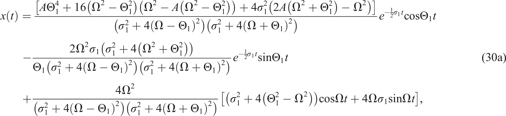
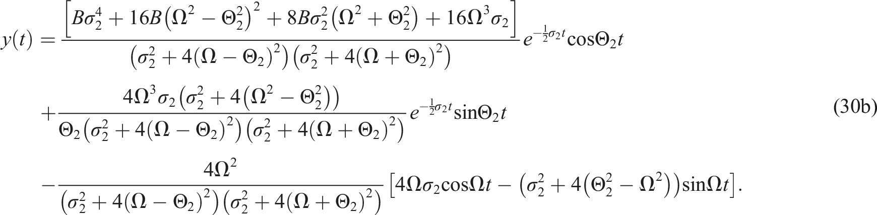
To examine the influence of the external forces on the behavior of the coupled Duffing nonlinear oscillator defined by the system (1), the solution of the full system (7) is derived as given by equations (30a,b). The graphing of these solutions together with the numerical solutions of the original system (1) is designed to allow studying the non-homogeneous system (7). The non-harmonic resonance case is desired when the exciting frequency $\mathrm{\Omega }$ is away from any primary frequencies ${\omega }_{10}^2\&{\omega }_{20}^2$ or away from the conservative frequencies ${\mathrm{\Theta }}_1$ and ${\mathrm{\Theta }}_2$ . In the graphed solutions (32-a,b), the forced frequency $\mathrm{\Omega }$ has been selected to be arbitrary and satisfy the non-harmonic resonance case. The calculations are done in the same system as given in Figure 1, choosing $\mathrm{\Omega }=0.7$ . The results of the numerical solution and the analytical solutions (32-a,b) are demonstrated in Figure 6, where ${\sigma }_1=0.21861,{\sigma }_2=0.324682, {\mathrm{\Theta }}_1=1.00797$ and ${\mathrm{\Theta }}_2=1.22357$ . The investigation of this figure reveals that the amplitude-time curves have a disturbance, where the amplitudes have jumped relatively to larger values. Further, it is observed that the wavelength is not fixed. It is also observed that the presence of $\mathrm{\Omega }$ has relatively suppressed the effect of the decaying rule of the damping coefficients.

Figure 6.

Perturbation solutions (30-a,b) (dotted red line) with the corresponding numerical solution of the forced system (1) (solid blue and green lines) for the same system given in Figure 1 with arbitrary $\mathrm{\Omega }=0.7$ .

If the harmonic resonance cases are considered, then there are some cases of how $\mathrm{\Omega }$ approaches the natural frequencies ${\omega }_{10}$ , ${\omega }_{20}$ and their combinations. The first case can be studied when $\mathrm{\Omega }$ is chosen to be near the linear frequency ${\omega }_{10}$ . This nearness is defined as $\mathrm{\Omega }={\omega }_{10}+{\epsilon }_1$ , where ${\epsilon }_i$ is called the detuning parameter. This parameter makes the analytical solutions very closer to the numerical results. The second harmonic resonance case is similar to the first case except that ${\omega }_{10}$ has been replaced by ${\omega }_{20}$ and ${\epsilon }_1$ replaced by ${\epsilon }_2$ . In the third case, $\mathrm{\Omega }=\frac{1}{2}\left({\omega }_{10}+{\omega }_{20}\right)+{\epsilon }_3$ , and finally in the fourth case $\mathrm{\Omega }=\frac{1}{2}\left({\omega }_{10}-{\omega }_{20}\right)+{\epsilon }_4$ . These four cases are demonstrated in Figure 7, Figure 8, Figure 9, and Figure 10. The suitable detaining parameter ${\epsilon }_i$ is found to be ${\epsilon }_1=-0.4$ , ${\epsilon }_3=-0.5$ and ${\epsilon }_4=-0.5$ . The major observation is that the analytical solutions (30-a,b) have an excellent agreement, even in the presence of the periodic forces. In these cases, the system will oscillate, but its amplitude gradually decreases until it rests.

Figure 7.

Perturbation solutions with the corresponding numerical solution in the harmonic resonance case of $\mathrm{\Omega }$ = ${\omega }_{10}+{\epsilon }_1$ for the same system given in Figure 1. The detuning parameter is ${\epsilon }_1=-0.4$ .

Figure 8.

Perturbation solutions with the corresponding numerical solution in the harmonic resonance case of $\mathrm{\Omega }$ = ${\omega }_{20}+{\epsilon }_2$ for the same system given in Figure 1. The detuning parameter is ${\epsilon }_2=-0.7$ .

Figure 9.

Perturbation solutions with the corresponding numerical solution in the harmonic resonance case of $\mathrm{\Omega }$ = $\frac{1}{2}\left({\omega }_{10}+{\omega }_{20}\right)+{\epsilon }_3$ for the same system given in Figure 1. The detuning parameter is ${\epsilon }_3=-0.5$ .

Figure 10.

Perturbation solutions with the corresponding numerical solution in the harmonic resonance case of $\mathrm{\Omega }$ = $\frac{1}{2}\left({\omega }_{10}-{\omega }_{20}\right)+{\epsilon }_4$ for the same system given in Figure 1. The detuning parameter is ${\epsilon }_4=-0.5$ .

The harmonic nonlinear resonance cases

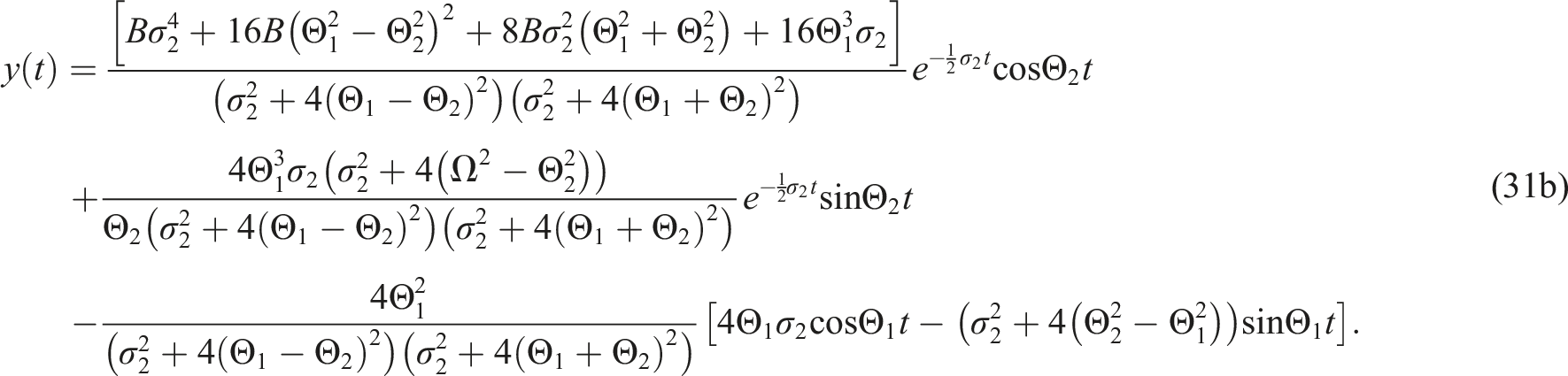
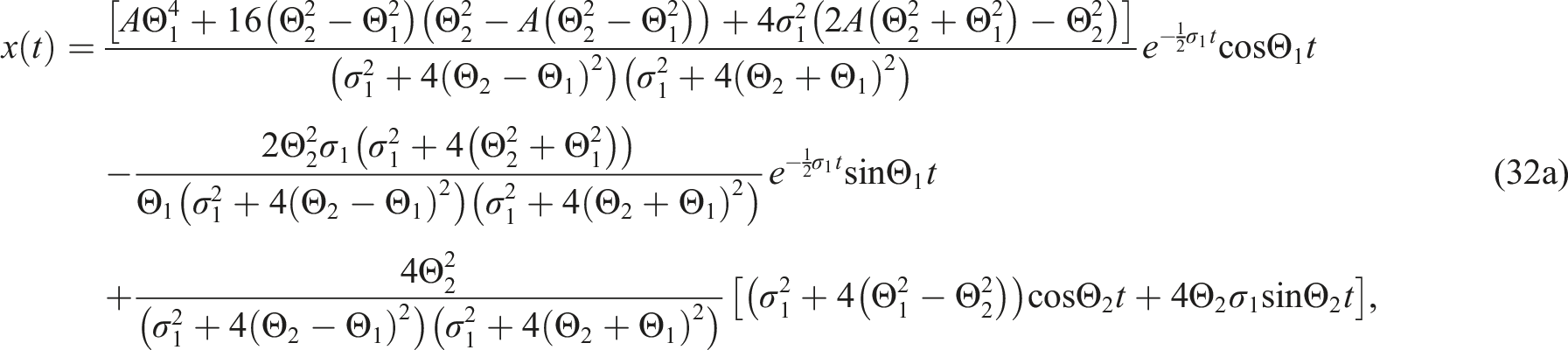
As the non-conservative frequencies ${\mathrm{\Theta }}_1$ and ${\mathrm{\Theta }}_2$ are analytically obtained, then the nonlinear harmonic resonance cases will be discussed only for the analytical solutions, where the numerical solutions in the present resonance cases will not be covered. To this end, the solutions (30-a,b) in the case of $\mathrm{\Omega }\to {\mathrm{\Theta }}_1$ becoming

$x\left(t\right)=\frac{{\mathrm{\Theta }}_1^2}{{\sigma }_1^2\left({\sigma }_1^2+16{\mathrm{\Theta }}_1^2\right)}\left[\left(A\left({\mathrm{\Theta }}_1^2+4{\sigma }_1^2\right)-4{\sigma }_1^2\right)e^{-\frac{1}{2}{\sigma }_{1}t}+4{\sigma }_1^2\right]\cos {\mathrm{\Theta }}_{1}t-\frac{2{\mathrm{\Theta }}_1}{{\sigma }_1\left({\sigma }_1^2+16{\mathrm{\Theta }}_1^2\right)}\left[\left({\sigma }_1^2+8{\mathrm{\Theta }}_1^2\right)e^{-\frac{1}{2}{\sigma }_{1}t}-8{\mathrm{\Theta }}_1^2\right]\sin {\mathrm{\Theta }}_{1}t,$

(31a)

$\begin{array}{l}y\left(t\right)=\frac{\left[B{\sigma }_2^4+16B{\left({\mathrm{\Theta }}_1^2-{\mathrm{\Theta }}_2^2\right)}^2+8B{\sigma }_2^2\left({\mathrm{\Theta }}_1^2+{\mathrm{\Theta }}_2^2\right)+16{\mathrm{\Theta }}_1^3{\sigma }_2\right]}{\left({\sigma }_2^2+4{\left({\mathrm{\Theta }}_1-{\mathrm{\Theta }}_2\right)}^2\right)\left({\sigma }_2^2+4{\left({\mathrm{\Theta }}_1+{\mathrm{\Theta }}_2\right)}^2\right)}{e}^{-\frac{1}{2}{\sigma }_{2}t}\cos {\mathrm{\Theta }}_{2}t\\ +\frac{4{\mathrm{\Theta }}_1^3{\sigma }_2\left({\sigma }_2^2+4\left({\mathrm{\Omega }}^2-{\mathrm{\Theta }}_2^2\right)\right)}{{\mathrm{\Theta }}_2\left({\sigma }_2^2+4{\left({\mathrm{\Theta }}_1-{\mathrm{\Theta }}_2\right)}^2\right)\left({\sigma }_2^2+4{\left({\mathrm{\Theta }}_1+{\mathrm{\Theta }}_2\right)}^2\right)}{e}^{-\frac{1}{2}{\sigma }_{2}t}\sin {\mathrm{\Theta }}_{2}t\\ -\frac{4{\mathrm{\Theta }}_1^2}{\left({\sigma }_2^2+4{\left({\mathrm{\Theta }}_1-{\mathrm{\Theta }}_2\right)}^2\right)\left({\sigma }_2^2+4{\left({\mathrm{\Theta }}_1+{\mathrm{\Theta }}_2\right)}^2\right)}\left[4{\mathrm{\Theta }}_1{\sigma }_2\cos {\mathrm{\Theta }}_{1}t-\left({\sigma }_2^2+4\left({\mathrm{\Theta }}_2^2-{\mathrm{\Theta }}_1^2\right)\right)\sin {\mathrm{\Theta }}_{1}t\right].\end{array}$

(31b)

In the case of $\mathrm{\Omega }\to {\mathrm{\Theta }}_2$ , the analytical solution yields

$\begin{array}{l}x\left(t\right)=\frac{\left[A{\mathrm{\Theta }}_1^4+16\left({\mathrm{\Theta }}_2^2-{\mathrm{\Theta }}_1^2\right)\left({\mathrm{\Theta }}_2^2-A\left({\mathrm{\Theta }}_2^2-{\mathrm{\Theta }}_1^2\right)\right)+4{\sigma }_1^2\left(2A\left({\mathrm{\Theta }}_2^2+{\mathrm{\Theta }}_1^2\right)-{\mathrm{\Theta }}_2^2\right)\right]}{\left({\sigma }_1^2+4{\left({\mathrm{\Theta }}_2-{\mathrm{\Theta }}_1\right)}^2\right)\left({\sigma }_1^2+4{\left({\mathrm{\Theta }}_2+{\mathrm{\Theta }}_1\right)}^2\right)}{e}^{-\frac{1}{2}{\sigma }_{1}t}\cos {\mathrm{\Theta }}_{1}t\\ -\frac{2{\mathrm{\Theta }}_2^2{\sigma }_1\left({\sigma }_1^2+4\left({\mathrm{\Theta }}_2^2+{\mathrm{\Theta }}_1^2\right)\right)}{{\mathrm{\Theta }}_1\left({\sigma }_1^2+4{\left({\mathrm{\Theta }}_2-{\mathrm{\Theta }}_1\right)}^2\right)\left({\sigma }_1^2+4{\left({\mathrm{\Theta }}_2+{\mathrm{\Theta }}_1\right)}^2\right)}{e}^{-\frac{1}{2}{\sigma }_{1}t}\sin {\mathrm{\Theta }}_{1}t\\ +\frac{4{\mathrm{\Theta }}_2^2}{\left({\sigma }_1^2+4{\left({\mathrm{\Theta }}_2-{\mathrm{\Theta }}_1\right)}^2\right)\left({\sigma }_1^2+4{\left({\mathrm{\Theta }}_2+{\mathrm{\Theta }}_1\right)}^2\right)}\left[\left({\sigma }_1^2+4\left({\mathrm{\Theta }}_1^2-{\mathrm{\Theta }}_2^2\right)\right)\cos {\mathrm{\Theta }}_{2}t+4{\mathrm{\Theta }}_2{\sigma }_1\sin {\mathrm{\Theta }}_{2}t\right],\end{array}$

(32a)

$y\left(t\right)=\frac{1}{{\sigma }_2\left({\sigma }_2^2+16{\mathrm{\Theta }}_2^2\right)}\left[e^{-\frac{1}{2}{\sigma }_{2}t}\left(B{\sigma }_2^3+16B{\sigma }_2{\mathrm{\Theta }}_2^2+16{\mathrm{\Theta }}_2^3{\sigma }_2\right)-16{\mathrm{\Theta }}_2^3\right]\cos {\mathrm{\Theta }}_{2}t+\frac{4{\mathrm{\Theta }}_2^2}{\left({\sigma }_2^2+16{\mathrm{\Theta }}_2^2\right)}\left({\sigma }_2{e}^{-\frac{1}{2}{\sigma }_{2}t}+1\right)\sin {\mathrm{\Theta }}_{2}t.$

(32b)

In the case of $\mathrm{\Omega }$ approach ${\mathrm{\Theta }}_1={\mathrm{\Theta }}_2=\mathrm{\Theta }$ , the analytical solution yields

$x\left(t\right)=\frac{{\mathrm{\Theta }}^2}{{\sigma }_1^2\left({\sigma }_1^2+16{\mathrm{\Theta }}^2\right)}\left(\left(A{\mathrm{\Theta }}^2+4{\sigma }_1^2\left(4A-1\right)\right)e^{-\frac{1}{2}{\sigma }_{1}t}+4{\sigma }_1^2\right)\cos \mathrm{\Theta }t-\frac{2\mathrm{\Theta }{\sigma }_1}{{\sigma }_1^2\left({\sigma }_1^2+16{\mathrm{\Theta }}^2\right)}\left(\left({\sigma }_1^2+8{\mathrm{\Theta }}^2\right)e^{-\frac{1}{2}{\sigma }_{1}t}-8{\mathrm{\Theta }}^2\right)\sin \mathrm{\Theta }t,$

(33a)

$y\left(t\right)=\frac{1}{{\sigma }_2\left({\sigma }_2^2+16{\mathrm{\Theta }}^2\right)}\left(\left(B{\sigma }_2^3+16B{\sigma }_2{\mathrm{\Theta }}^2+16{\mathrm{\Theta }}^3\right)e^{-\frac{1}{2}{\sigma }_{2}t}-16{\mathrm{\Theta }}^3\right)\cos \mathrm{\Theta }t+\frac{4{\mathrm{\Theta }}^2}{\left({\sigma }_2^2+16{\mathrm{\Theta }}^2\right)}\left({\sigma }_2{e}^{-\frac{1}{2}{\sigma }_{2}t}+1\right)\sin \mathrm{\Theta }t.$

(33b)

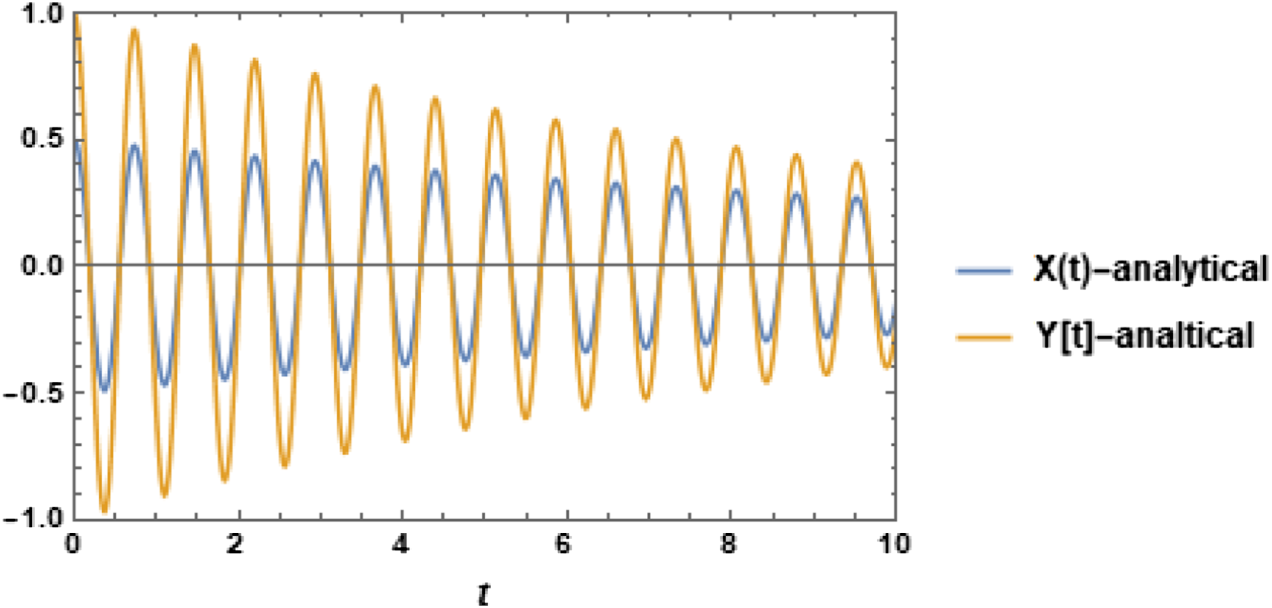
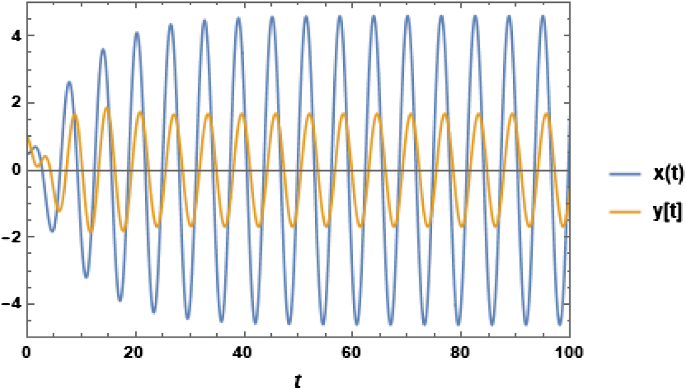
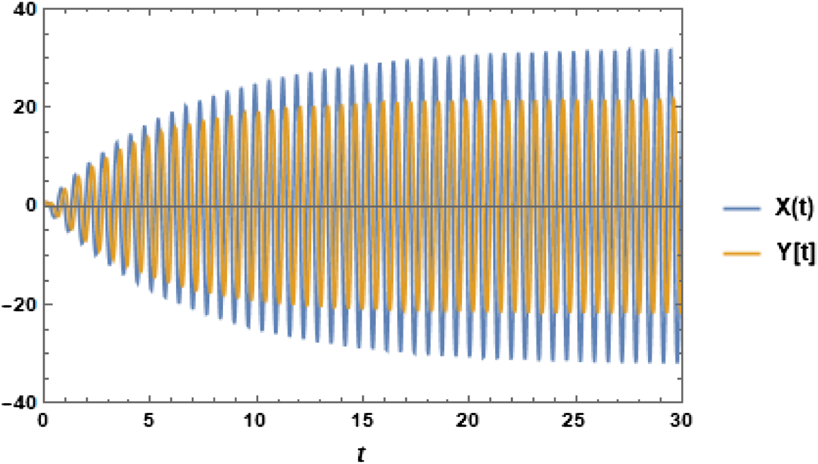
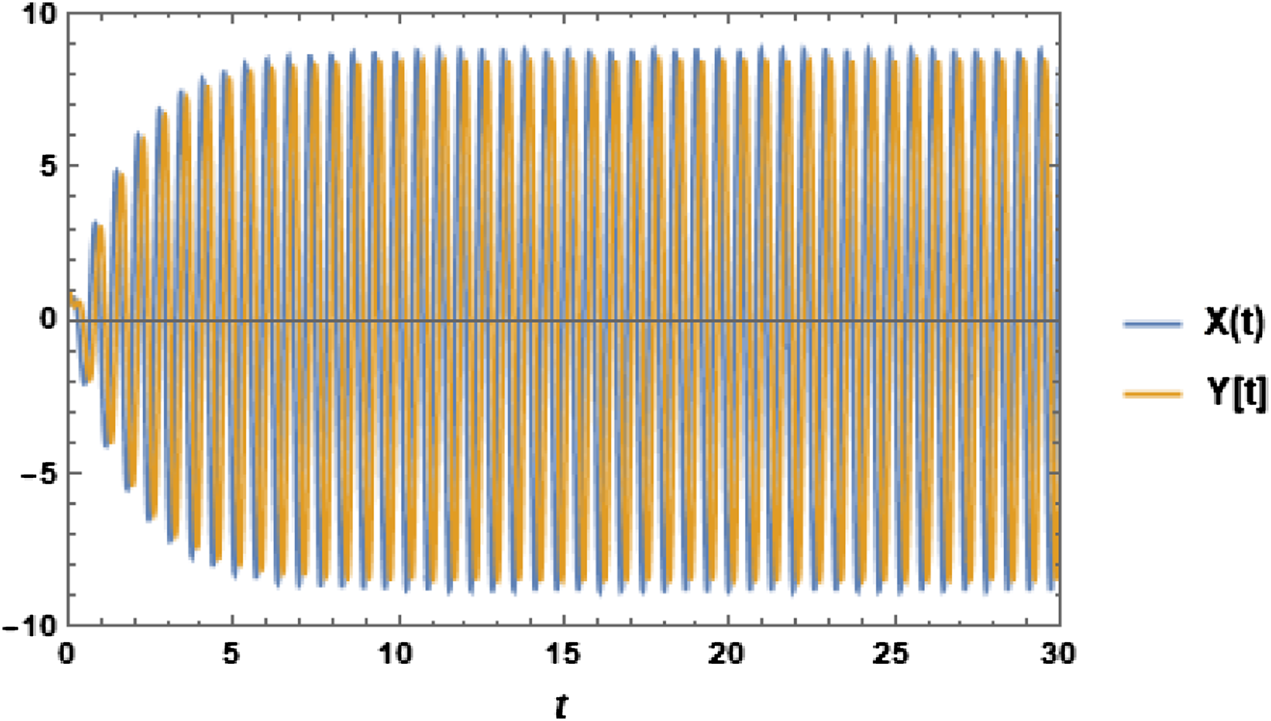
The approaching of the forced frequency $\mathrm{\Omega }$ to the non-conservative frequencies ${\mathrm{\Theta }}_1$ and ${\mathrm{\Theta }}_2$ has been graphed and displayed in Figure 11 in the case $\mathrm{\Omega }={\mathrm{\Theta }}_1$ and $\mathrm{\Omega }={\mathrm{\Theta }}_2$ , respectively. The calculations have been done for the analytical solutions (31-a,b) and (32-a,b). It is shown that both amplitude-time curves have increased to a specific larger value and oscillated at a fixed value so that periodic solutions can be revealed over time. The amplitude-time curve $x\left(t\right)$ is larger than the amplitude-time curve $x\left(t\right)$ as shown in Figure 11, while in Figure (12), the opposite case is observed. These behaviors indicate that the application of the periodic force to the nonlinear harmonic cases has suppressed the influence of decaying parameters ${\sigma }_1$ and ${\sigma }_2$ . In addition, the periodic behavior will continue without damping. The graph in Figure 13 is concerned with the analytical solution (35-a,b), where the case $\mathrm{\Omega }={\mathrm{\Theta }}_1={\mathrm{\Theta }}_2$ is considered for the same system given in Figure 1. It shows that the wave-time amplitude has gradually increased to a high value and then has a constant magnitude so that the periodic behavior can be disclosed. This high amplitude can be suppressed by increasing the damping coefficients as displayed in Figure 14. When non-weak damping is present, the general picture does not change much, but small amplitudes are gained. It is noted that the height of the amplitude-time wave has decreased when ${\mu }_1=1$ and ${\mu }_2=1$ . Also, the wavelength has decreased as the linear damping coefficient increases. The graph shows that the amplitude does not decrease further, and never stops oscillating, and behaves like an undamped system. The periodic behavior observed in these graphs occurs in the resonance cases and is due to applying the external periodic forces. In the absence of external forces, the system will oscillate and gradually stop due to frictional damping.

Figure 11.

The graph for the solutions (31-a,b) at the harmonic resonance case of $\mathrm{\Omega }$ = ${\mathrm{\Theta }}_1$ for the same system is given in Figure 1.

Figure 12.

The graph for the solutions (32-a,b) at the harmonic resonance case of $\mathrm{\Omega }$ = ${\mathrm{\Theta }}_2$ for the same system is given in Figure 1.

Figure 13.

The graph for the solutions (33-a,b) at the harmonic resonance case of $\mathrm{\Omega }={\mathrm{\Theta }}_1={\mathrm{\Theta }}_2$ , for the same system is given in Figure 1.

Figure 14.

The graph for the solutions (33-a,b) at the harmonic resonance case of $\mathrm{\Omega }={\mathrm{\Theta }}_1={\mathrm{\Theta }}_2$ , for the same system given in Figure 1 except that ${\mu }_1={\mu }_2=1$ .

Conclusion

Without using perturbation techniques, a novel method of identification of the damping nonlinear coupled oscillations has been proposed. It is mainly based on obtaining an equivalent linear damping system. Each equation has a new damping coefficient, which is estimated depending on all the linear and nonlinear damping effects of the original system. The non-conservative frequency for each equation is achieved. The resulting linear system has an exact solution containing coefficients performed in terms of the original coefficients of the coupled nonlinear oscillators. The exact solutions are performed in both forced and unforced systems. In the unforced system, two kinds of self-resonances are distinguished. The internal resonance case and the nonlinear resonance case are discussed and compared with the numerical solutions. Further, the harmonic resonance cases approaching the frequency of the periodic force to each natural frequency and their combinations are discussed and compared with the numerical solutions. The harmonic resonance case arising as the applied frequency approaches the analytical non-conservative frequencies is illustrated and studied. We have demonstrated how the two degrees of freedom dynamical equations may be solved analytically with an excellent agreement with the numerical solutions. We think that this approach approximates the exact solution quickly and has great potential, and then can be applied to other non-conservative nonlinear oscillators. Therefore, we can conclude that the quasi exact method is more available and effective.