
Abstract
Large redundant metal structures have high stability with large cost. An excellent mechanical structure should have the lower weight when satisfying its stability. Aiming at the large redundancy of the main beam metal structure of the double-beam bridge crane, the paper extracts six important parameters to determine its quality, and the corresponding value is set. The orthogonal test table is designed to calculate the strength and stiffness. In order to avoid resonance, the fixed vibration frequency and excitation frequency are calculated. The experimental results are fitted to obtain the six parameters of the quality, strength, stiffness, and natural frequency. Moreover, particle swarm optimization algorithm is used to solve the multi-objective optimization mathematical model with the design quality as the goal and the stiffness, strength, and easy resonance interval as constraints. In view of the long calculation time and poor convergence of particle swarm optimization algorithm, a module that limits the particle forward speed is added and the generation conditions of particles are redefined. The improved particle swarm algorithm shows that the first-order vibration frequency of the main beam increases from 18 Hz to 27.55 Hz. It improves the stability of the overall structure and avoids resonance with the motor frequency. Under the condition of satisfying the stability of the main beam, the quality of the main beam is reduced from 1.23 tons to 0.53 tons, with a reduction of 6%.
Keywords
Introduction
Bridge crane is an important lifting and handling equipment that widely used in heavy machinery workshop. 1 Early mechanical structure design of cranes mostly relies on experience. In order to be safe, mechanical structures with large redundant coefficients are usually designed. 2 Metal structures with large redundancy tend to have optimal stability, and their cost is relatively high. This is a burden for heavy machinery manufacturers such as agricultural machinery and steelmaking industries, where cranes are in high demand. With the outbreak of the third industrial Revolution in the 1940s and 1950s, the high-tech industry represented by electronic computer technology rose rapidly. After decades of development, computers have been widely used in mechanical design and optimization. 3 Zhu and Liu 4 used HyperMesh pre-processing software and OptiStruct solver to optimize the main beam design of bridge cranes for multiple working conditions. Based on an embedded disturbance mechanism, Lu et al. 5 used an improved artificial fish swarm algorithm to optimize the main beam dosing of a bridge crane. Based on the finite element analysis of the strength, stiffness, and stability of the main beam of the overhead traveling crane, Yu et al. 6 used an intelligent optimization algorithm-mirror reflection algorithm to optimize the design parameters of the crane metal structure to reduce the quality of the structure.
The main beam of the overhead traveling crane is a box structure that contains several size factors. Each size will affect the strength and weight of the structure. In recent years, many optimization algorithms such as swarm algorithms and bat algorithms 7–8 are widely used in the optimization of crane structures. How to design the optimization algorithm and reduce the mass of the main beam by adjusting the parameters so as to ensure the stability of the structure in the state is the key idea of optimization. Based on the response surface method, the lightweight design of an open hydraulic pre-bending machine was carried out, and the quality of the pre-bending machine was reduced by 8330 kg after optimization. 9 Based on the same method, the lightweight design of the main beam of the bridge crane was carried out, and the quality of the main beam is reduced by 17% after optimization. Therefore, lightweight design reduces the quality under the premise of ensuring stability and has great economic benefits. 10
Aiming at the problems of low efficiency and low precision of traditional optimization methods in the structural optimization of the crane beam, a structural optimization method based on an improved particle swarm optimization algorithm is proposed. Under the condition of satisfying the deformation and stress, the structure is optimized and the lightweight design is carried out to reduce the production cost. Moreover, based on the original particle swarm algorithm, an improved particle swarm optimization algorithm is designed to improve the running speed and optimization effect. It can effectively ensure the stability of the structure and adjust various parameters to minimize the quality of the main beam.
First, the software SOLIDWORKS is used to establish the main beam, end beam, and car model of the crane. Second, the static mechanical analysis of the bridge crane is carried out to verify the structural stiffness in static state. Third, the modal analysis, weak part searching, optimal parameter selection, and orthogonal experiment design are carried out. Finally, the mathematical model is established, and the improved particle swarm optimization algorithm is used for fitting. On the basis of ensuring the dynamic and static performance, the quality of the main beam and the maximum deformation are reduced, and the natural frequency is improved. In addition, the performance of the whole machine is also improved accordingly.
Static mechanical analysis of the bridge crane
Introduction of the bridge crane structure
The drawing of a double-beam bridge crane in this study is the production drawing of a crane manufacturer in Changyuan City, Henan Province. The general assembly drawing is shown in Figure 1, and the main beam drawing is shown in Figure 2. General assembly drawing. Main girder drawing.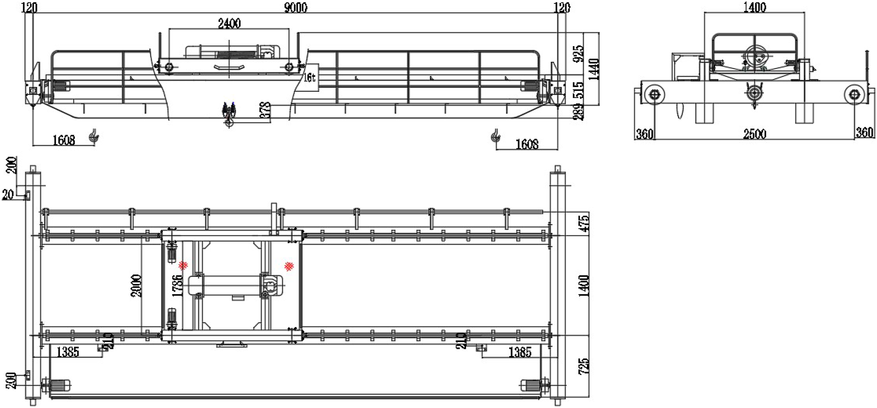
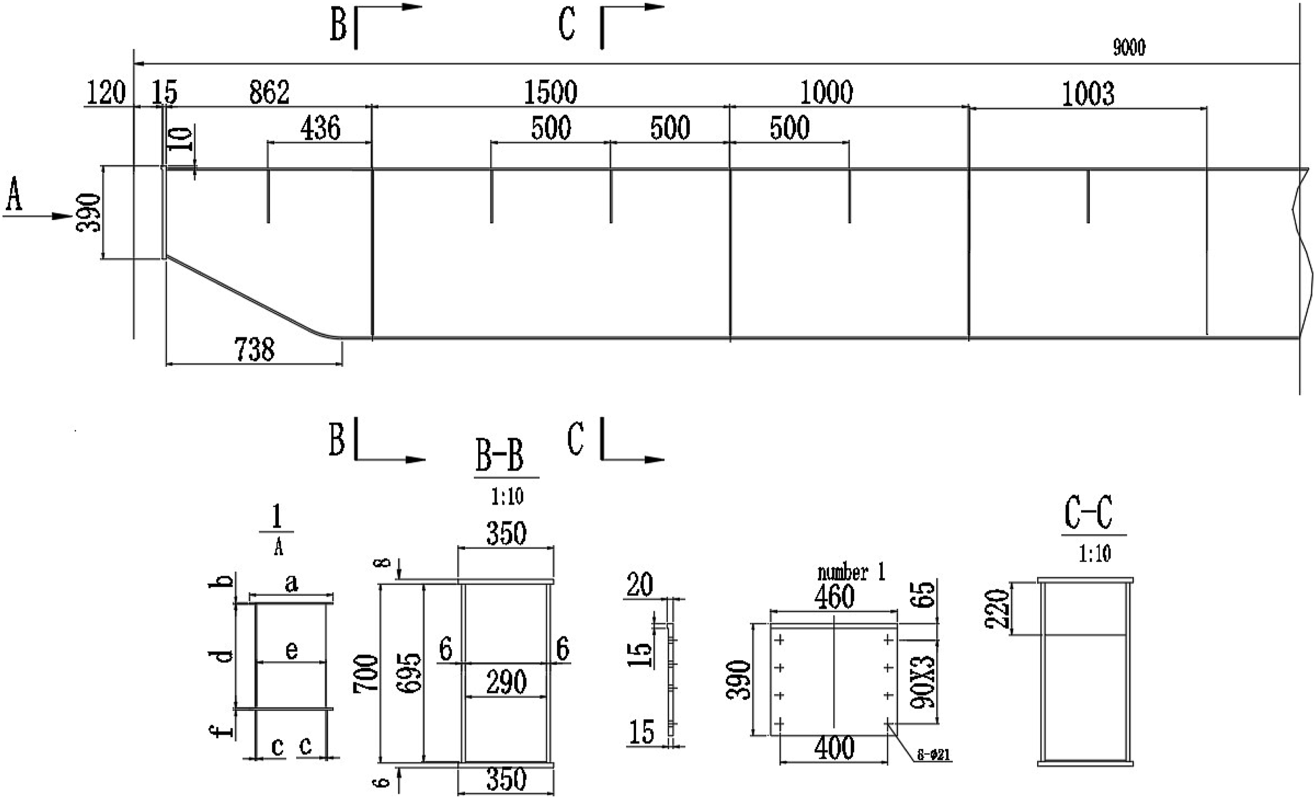
As the optimization target, the section size of the main beam structure is shown in Figure 3. The six parameters of the section are extracted, that is, the length of the upper wing is a; the thickness of the upper wing is b; the thickness of the web is c; the height of the web is d; the spacing between the two webs is e; and the thickness of the lower wing is f. Parameterization diagram of main beam section size.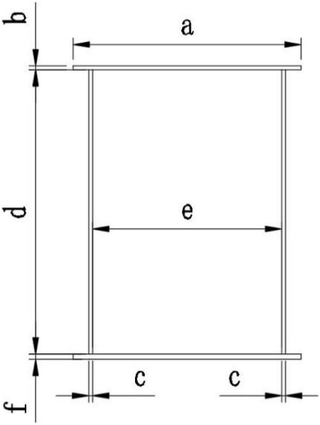
Static stiffness analysis of the bridge crane
The stiffness of crane structure can be divided into the static stiffness and the dynamic stiffness. In this section, this section mainly analyzes the static stiffness. The static stress analysis model of the main beam can be simplified into a simply supported beam model with fixed ends, as shown in Figure 4. Simplified diagram of main girder.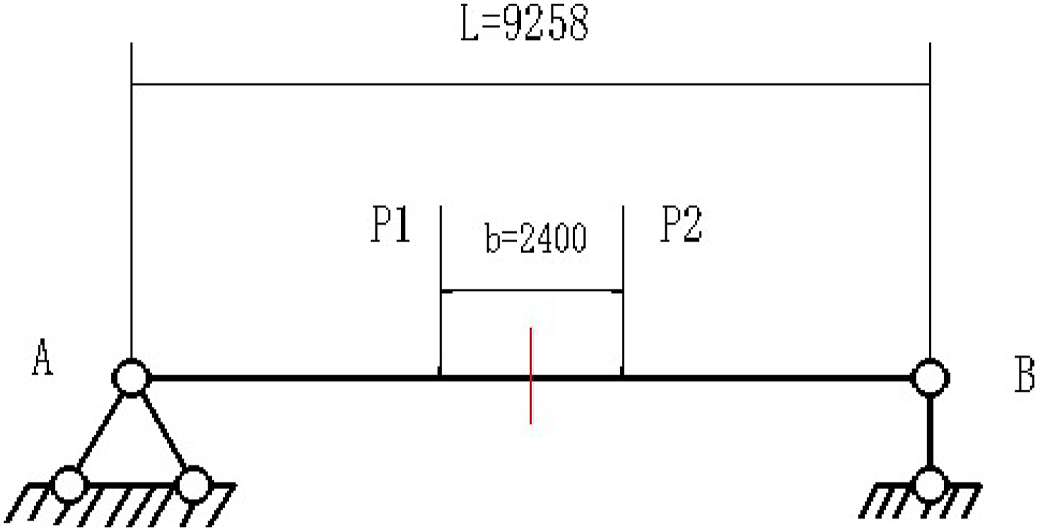
Aiming at the situation that the concentrated load is concentrated in the center, the effective stiffness method under the concentrated load is established. In this paper, the load is concentrated in the center of two symmetrical loads. Therefore, the two loads are equivalent to the loads at the midpoint. The calculation equation of the effective stiffness method needs to be modified, and the equivalent calculation equation of the static deflection theory can be used for calculation.
11
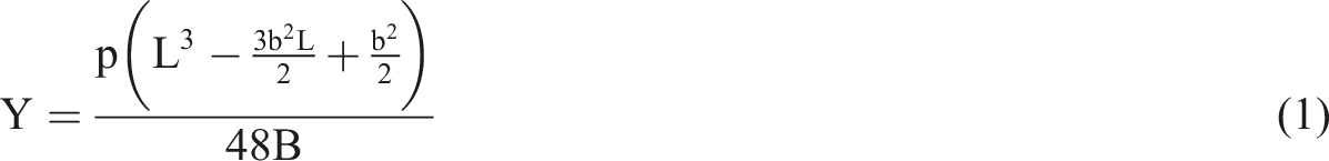
In equation (1),the sizes of L and B are shown in Figure 4. B is the effective stiffness of the section.
12
The effective stiffness calculation equation is defined as follows:

In equation (2), λ is the reduction coefficient in the range of 0–1, λ mainly considers the impact of shear deformation of web on stiffness.
According to the drawings, the three-dimensional drawing software SOLIDWORKS is used to accurately model the crane beam, end beam, and trolley. The general assembly diagram is shown in Figure 5. General assembly drawing.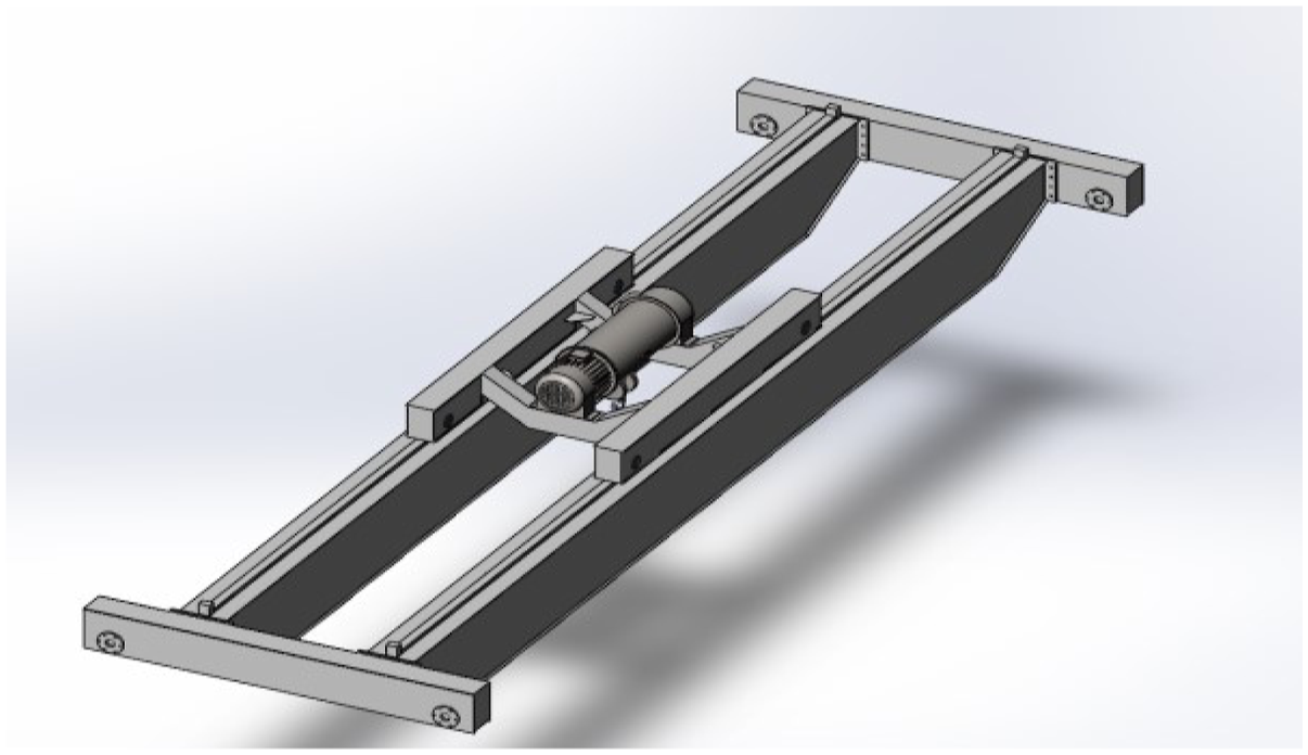
Using the quality evaluation function of SolidWorks, the mass of the main beam, end beam and trolley frame is 1.23 tons, 0.24 tons, and is 0.66 tons, respectively, it is 98% similar to the weight marked on the drawing.
Section parameters and deflection values of crane beam.
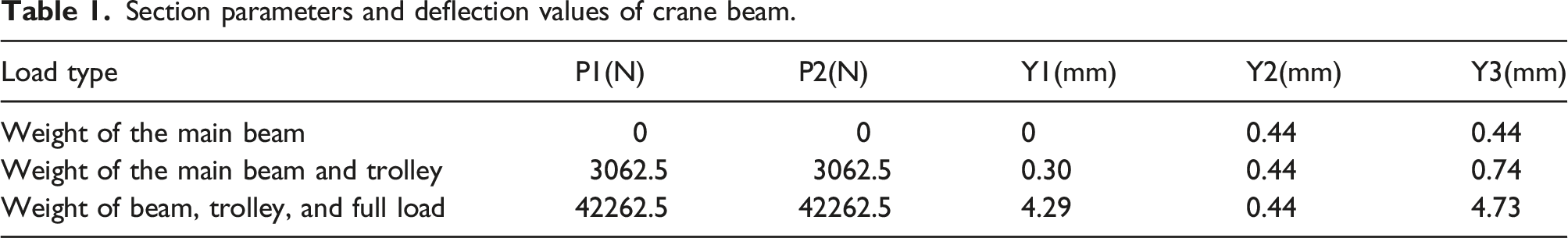
The dead weights of the single main beam and trolley running mechanism are 1.23 tons and 1.25 tons, respectively. The length of the upper wing plate is a = 350 mm; the thickness of the upper wing plate is B = 8 mm; the thickness of the web plate is C = 6 mm; the height of the web plate is D = 700 mm; the distance between the two webs is E = 290 mm; and the thickness of the lower wing plate is F = 6 mm. The distance in the longitudinal center plane of the beams at both ends is L = 9258 mm, and Q is 1964N/m under uniform distributed load.
Static strength analysis of the bridge crane
The stress concentration point near the center where the maximum stress may exist is selected for analysis. Three stress concentration points were selected for calculation. 13 The first is carried out on the lower edge Angle of the lower flange plate near the mid-span of the main beam. The second is carried out on the weld between the lower flange plate and the lower edge of the web near the mid-span of the main beam. The third is carried out on the upper edge of the web near the mid-span and the wheel pressure of the main beam and the wheel pressure.
The force diagram of the simply supported beams is established, as shown in Figure 6. Force diagram of the simply supported beam.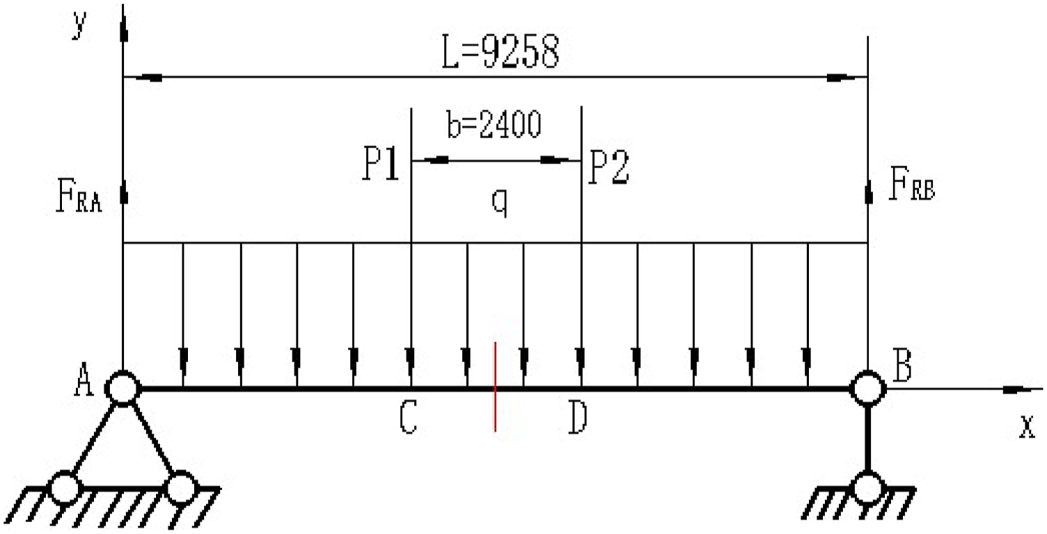
According to relevant knowledge of material mechanics, the equation of shear force and bending moment of this model is obtained as follows:
The shear force:
The bending moment:
The central section of the main beam X =4.629 is put into the above two equations when Fs=3064 N and M = 129903.17 N/m.
The maximum stress at the lower edge Angle of the lower flange plate near the mid-span of the main beam is calculated as:
The shear stress should be considered when calculating the strength of the second stress concentration point so that the static moment S
z
of the lower flange plate to the neutral axis should be calculated first. The static moment is the product of the area of a graph and its centroid to a coordinate axis, shown as equation (3).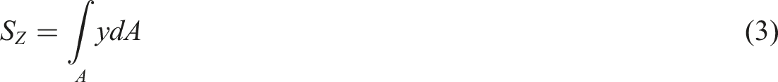
The shear stress of the section in equation (4)is as follows:
The shear stress at this point is calculated as follows:
According to the fourth strength theory, the total stress at this point is
The third stress concentration should not only consider the normal stress and shear stress but also the local compressive stress produced by the car wheel. The bending moment of point C, Mc = 153709.074 N/m and the shear force Fc = 41555 N are calculated according to the equations of shear force and moment. The normal stress and shear stress at this point are 
Substituting the data, it can be concluded that:
In this case, equation (6) can be obtained according to the combined stress theory
Substituting the data into equation (6), it can be obtained that
The third dangerous point also meets the strength requirements.
Vibration reliability analysis of the bridge structure
Modal analysis of the bridge structure
In order to prevent the bridge crane from resonating during operation, the modal m analysis of the bridge structure in Workbench is used for modal analysis.
16
The first-order modal analysis is shown in Figure 7. The first vibration mode of the bridge structure.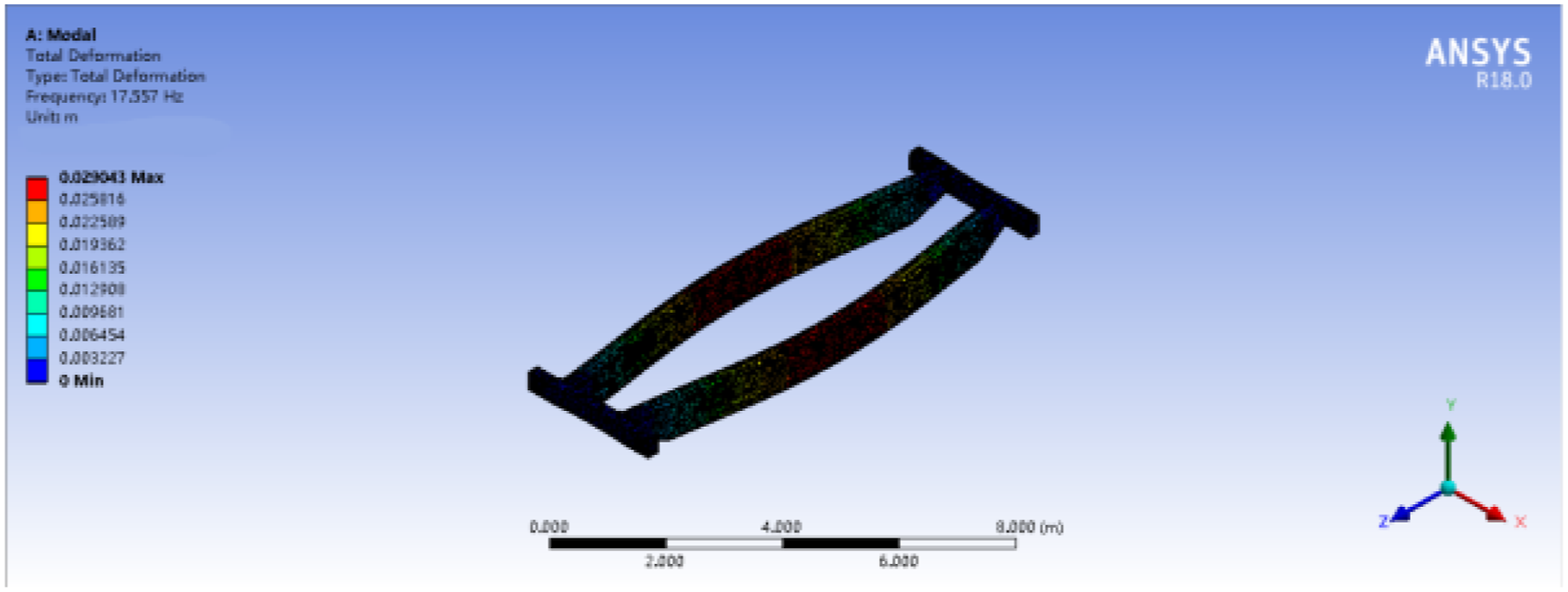
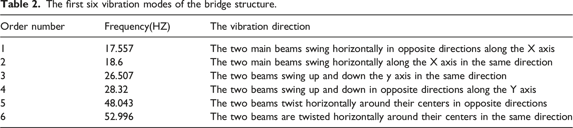
The first six vibration modes of the bridge structure.
Harmonic response analysis of bridge structure
Harmonic response analysis is mainly used to determine whether a metal structure can successfully overcome resonance-induced fatigue damage under successive cycles of external force. 17
Finite element analysis can be used to analyze the harmonic response of the structure. The vertical and horizontal frequency response curves are shown in Figure 8 and Figure 9, respectively. Vertical frequency response curve. Horizontal frequency response curve.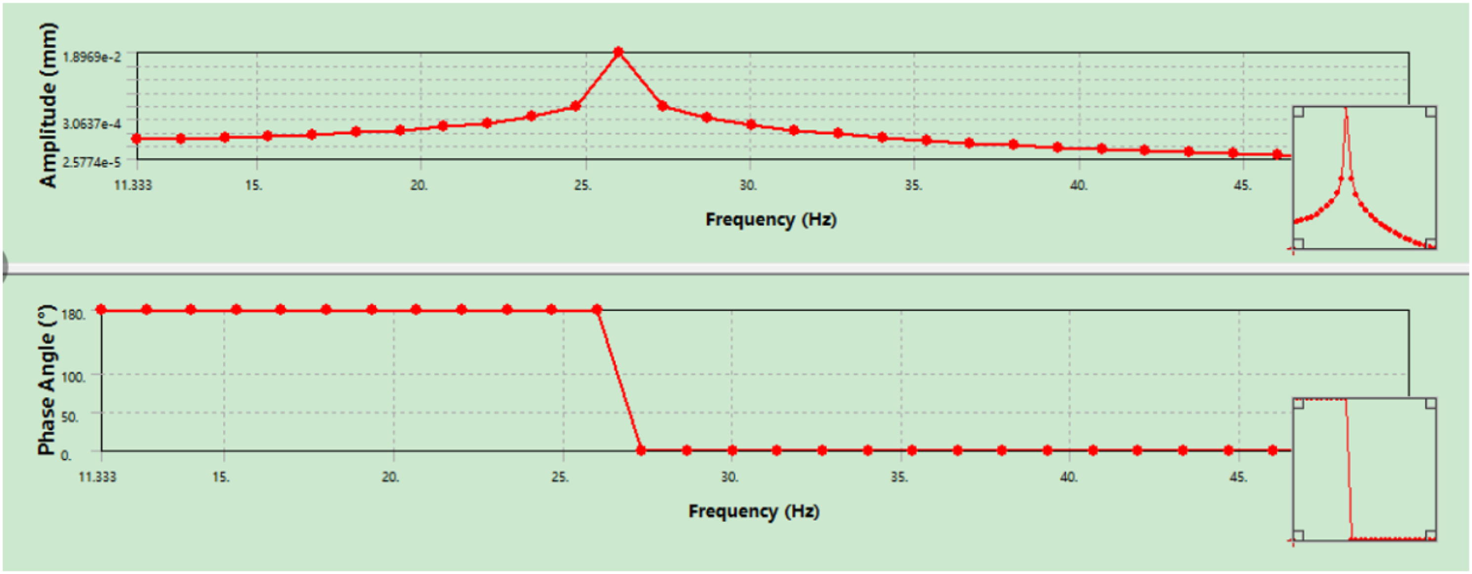
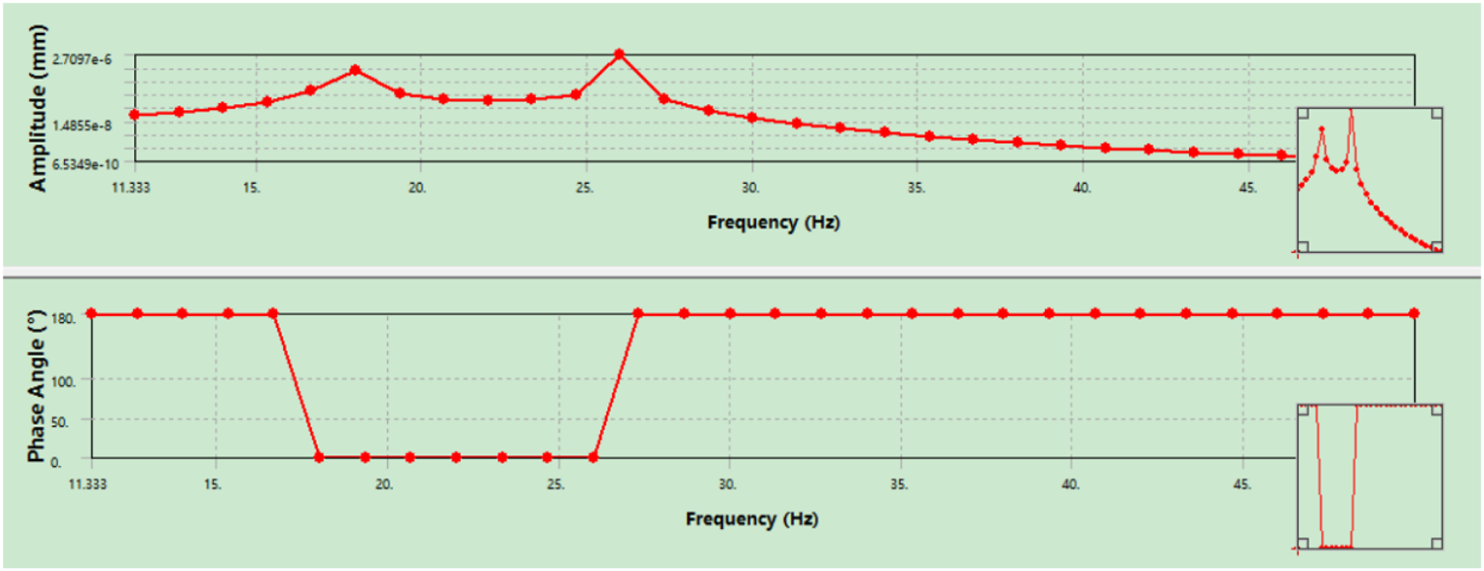
When the vibration frequency reaches 26 Hz, the amplitude reaches it speak and the mechanism vibrates violently. When the amplitude reaches 18 Hz and 26 Hz, the amplitude reaches it speak, and the mechanism produces severe left-right vibration, as shown in Figures 8 and 9. Therefore, motors around 18 Hz and 26 Hz should not be selected in the design or the natural vibration frequency of the designed structure should be away from 18 Hz and 28 Hz.
Optimization of key parts of the bridge crane
Determine the range of optimization parameters
According to the crane drawings of the upper wing length of 350 mm, and referring to the actual production of cranes, the lifting weight is 5 tons, and the crane girder width is about 10 centimeters. In order to guarantee the precision of the optimal solution, in the range of 10 cm, a value on the length of the wing is [300,400]; the thickness b of the upper wing is 3,10; the thickness c of the two webs is 3,10; the thickness d of the webs is [400,900]; the distance e between the two webs is [240,350]; and the thickness f of the lower wing is.3,10 On this basis, the design of subsequent experiments is carried out.
Design orthogonal experiment
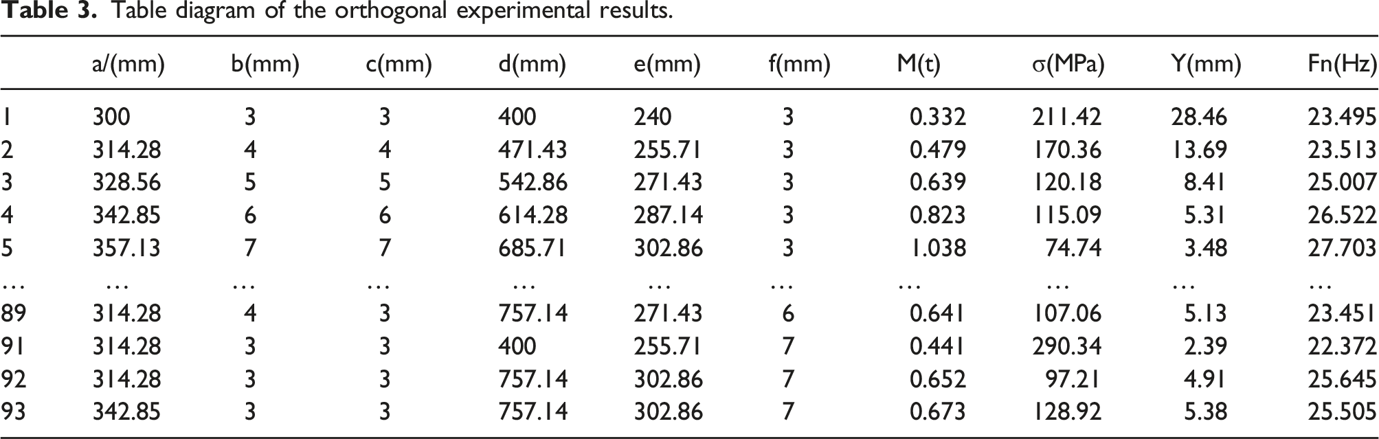
Table diagram of the orthogonal experimental results.
Acquisition and analysis of experimental results
A total of 93 groups of experiments are required for this orthogonal test table, as shown in Table 3. The quality is calculated by SOLIDWORKS with the above mentioned method, and the maximum stress and deformation are calculated by the above finite element analysis method. The similar solid vibration frequencies are obtained by the above modal analysis and harmonic response analysis. The experimental results are filled in Table 3, and the orthogonal experimental results are also shown in Table 3.
It can be seen from Table 3 that the quality, the maximum stress, maximum deformation, and natural vibration frequency of the main beam under load have a certain relationship with the six structural parameters. But the greatest influencing factors on the quality, the maximum stress, the maximum deformation, and the natural vibration frequency can only be drawn after analyzing the orthogonal experimental results.
Regression fitting is performed on the test results by MATLAB.
19
The scatter diagram of mass M with respect to the independent variable is obtained, as shown in Figure 10. Scatter diagram of the independent variables in M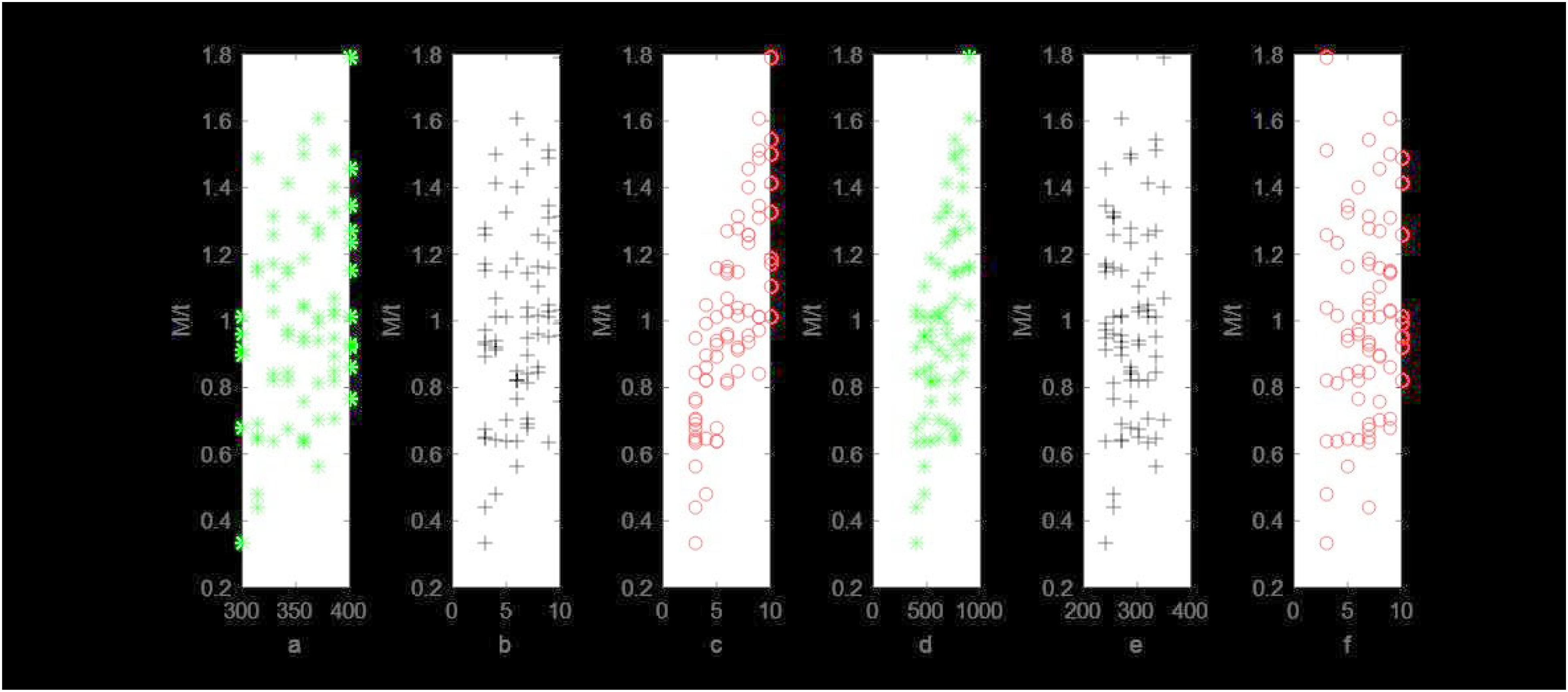
The distribution of mass M relative to all factors can be roughly expressed linearly, as shown in Figure 10. So it is linearly fitted to obtain a fitting equation: Residual diagram of M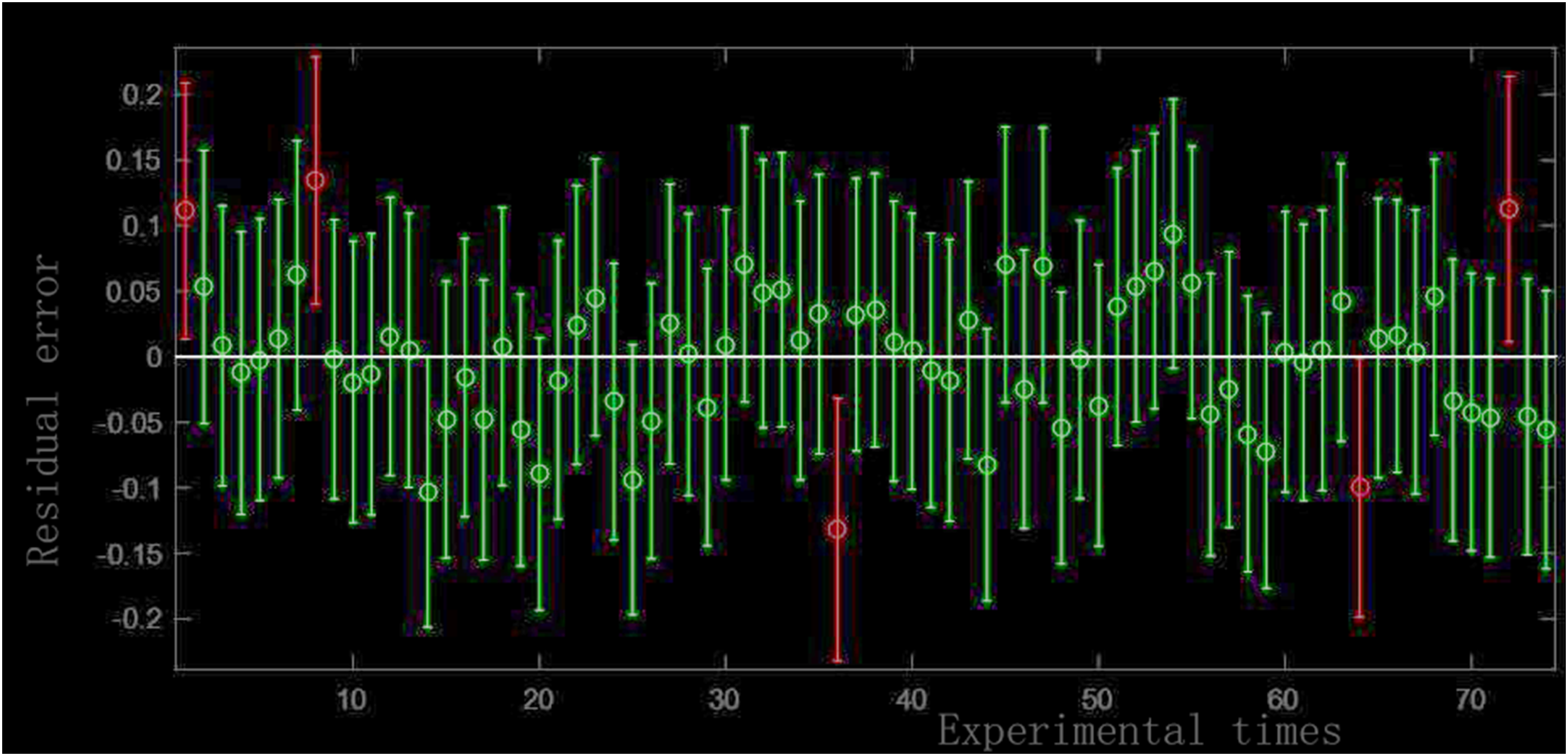
In Figure 11, only a few points have large residuals, and the residuals of other test points meet the requirements, indicating a good degree of fitting. In the same way, the regression analysis is performed on the maximum stress σ, maximum deformation Y, and the solid vibration frequency Fn in the same direction, and the fitting is obtained as follows:
Analysis and optimization of the mathematical model
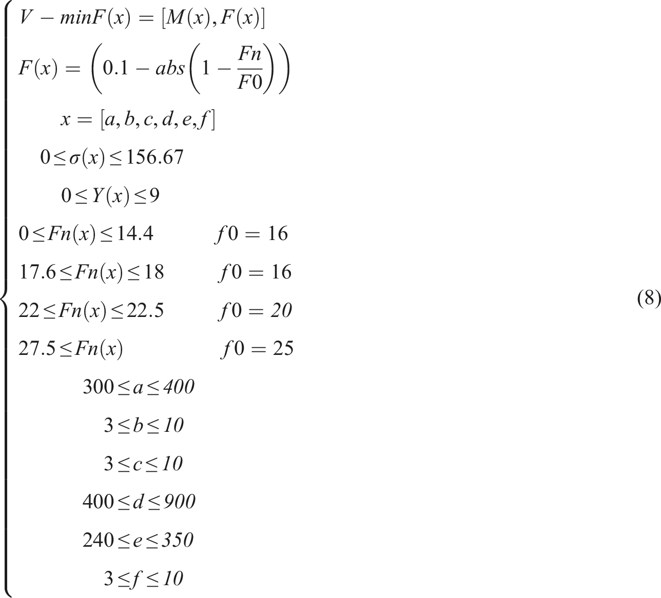
The optimization of the mathematical model generally consists of three parts: optimization objective, design variables, and constraint conditions. Using this mathematical model, the multi-condition discrete variable optimization problem can be transformed into a multi-objective and multi-constraint optimization problem.
20
The following is the three parts of the determination. 1. Determination of the objective function. It can be seen from the above, the study aims to make the main beam has lighter weight while ensuring the stability of the structure. Therefore, the main beam mass M is the first objective function. After optimization, it is also necessary to ensure that the natural frequency is far away from the excitation frequency. It is defined that the ratio of solid vibration frequency Fn to the excitation frequency F0 is between 0.9 and 1.1 and the resonance is strong so that the ratio should be as far as away from the range.
21
Then the dual problem can be expressed as follows: 2. Determination of the design variables. It can be seen from the above, the design variables are the upper wing length a, the upper wing thickness b, the web thickness c, the web height d, the spacing between the two webs e, and the thickness of the lower wing f. 3. Determination of the constraint conditions. It can be seen from the above, there are many constraint conditions in this paper, including the value range of variables a, b, c, d, e, and f, and the limit range of σ and Y, respectively. From Table 3, the variables a, b, c, d, e, and f is in the range of [300,400], [3,10], [3,10] [400,900], [240,350], and [3,10], respectively. If the safety factor of the mechanism is 1.5, the metal structure is Q235 B, and the yield stress σs is 235 MPa. The allowable stress is156.67 MPa, and the limit range of σ is 0 < σ ≤ 156.67 MPa. The bridge crane is lifting equipment with high accuracy requirements, and its deflection is required to be less than 1/1000. Since the span of the main beam is 9m, its maximum allowable deformation is 9 mm, and its maximum deformation range is 0 < Y ≤ 9 mm. For Fn, it is the solid vibration frequency with the same vibration direction and similar vibrations. The frequencies of the three vibration sources are 16 Hz, 20 Hz, and 25 Hz, respectively. When Fn is at (0,18) Hz, the limiting condition is 1.1 ≤ Fn/16 and Fn/16 ≤ 0.9. When Fn is between (18, 22.5), the limiting condition is 1.1 ≤ Fn/20 and Fn/20 ≤ 0.9. When Fn is between (22.5, ∞), the limiting condition is 1.1 ≤ Fn/25 and Fn/25 ≤ 0.9. Therefore, the value of Fn is in the range of (0,14.4) ∪ (17.6,18) ∪ (22,22.5) ∪ (27.5,∞).The mathematical model is established as equation (8):
Design of the optimization method
There are many algorithms for solving the multi-objective mathematical models, such as genetic algorithm,
22
particle swarm optimization,
23
fruit fly algorithm,
24
and ant colony algorithm.
25
This paper tends to use particle swarm optimization algorithm (PSO) to solve equation (8). In the PSO algorithm, different particles have individual fitness corresponding to the objective function, and each particle will be close to the optimal particle according to a specific law. When PSO is used to solve the constrained function optimization problems, it is often transformed into unconstrained optimization problems. Penalty functions are generally constructed by using the interior point penalty function method, and the expression of the penalty functions is as equation (9):

The main flow chart of improved particle swarm optimization is shown in Figure 12 Improved particle swarm algorithm flow chart.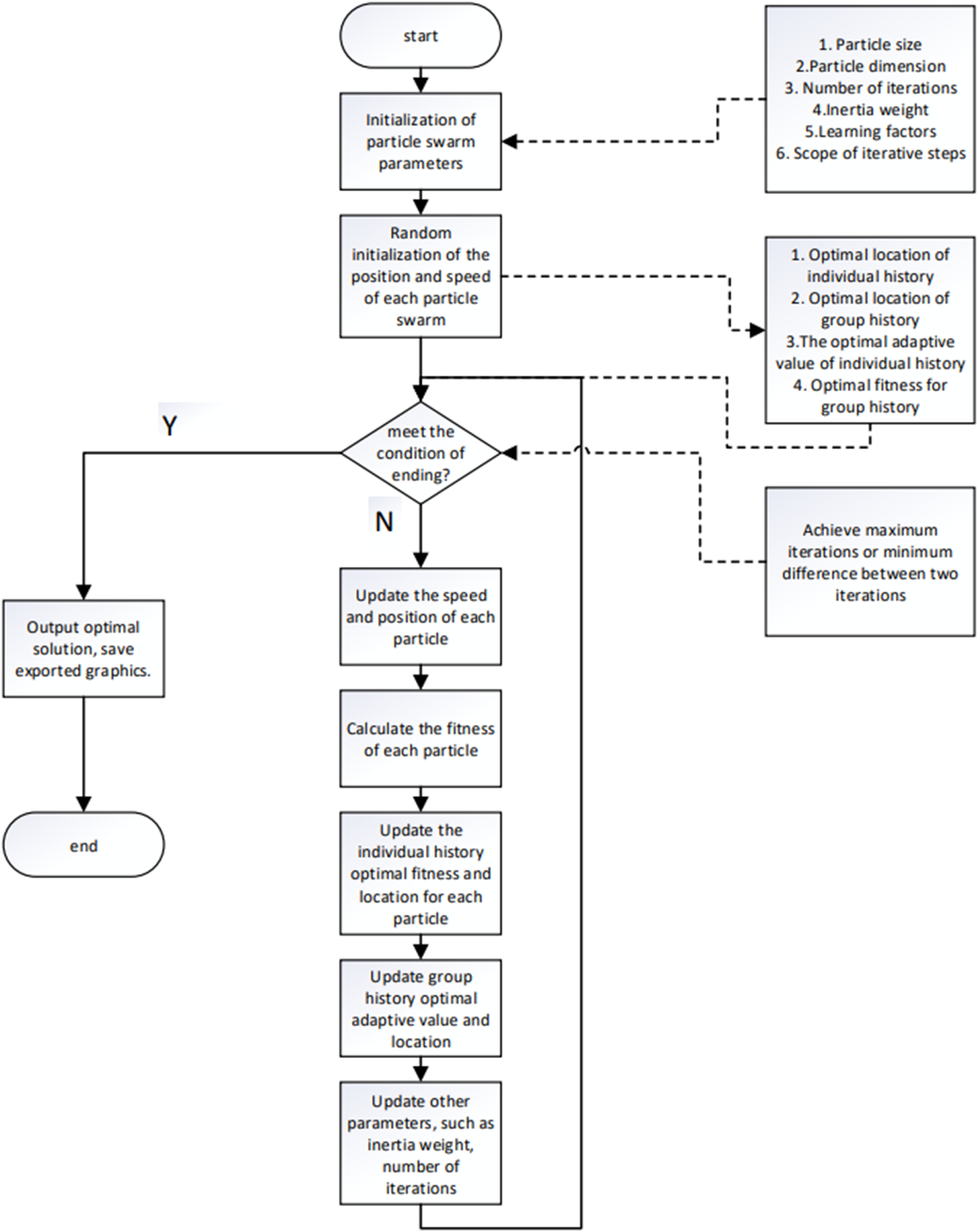
The calculation time of PSO algorithm increases with the increase of constraint functions and design variables. In this paper, there are 6 design variables and 16 constraint functions. Therefore, in the early stages of the algorithm, an approximate optimal solution by generating random numbers takes a long time and requires multiple runs. In order to solve the problem that PSO algorithm runs for a long time, and sometimes it is easy to fall into local optimal solution and cannot continue to iterate, the PSO algorithm is optimized.
During the optimization, there are two important conditions. The first is to have a sufficiently large particle swarm. The size of the result directly influences the quality of particle swarm optimization. If the particle swarms have small number, poor quality, high optimization starting point, and large optimal type of the local optimal solution in the later stage. The impact on the global optimization is also large and it is easy to find the optimal solution. The second is that the speed of the particles is appropriate, and the local optimization is obtained by setting the speed of particle swarm. If the speed is small, its optimal quality is high. If the speed is big, it is difficult to find the local optimal solution. Therefore, the right particle speed is the key to optimization. In order to optimize the original PSO algorithm, this paper first changes the way that the swarm finds the correct particles, replacing the original model of randomly generated particles. Then, the particle swarm that satisfies the constraints is converted into a particle swarm that first constrained and then judges whether each constraint is satisfied. This change will greatly improve the efficiency of obtaining suitable particles. Large quantities of high-quality particles can be obtained in a short time. This paper also adds a new function module to limit the forward speed of particles. This module aims to limit the speed of the particle swarm to a range that not too high, while maintaining its forward speed.
The original PSO algorithm is to optimize the multiple repeated operations of a small initial population, and the newly generated particle swarm has small cycles. If the initial population is more or the new particle swarm has a large number of loop traversals, the operation result is slow. The improved PSO algorithm limits the generation speed of new particles. It can carry out more initial population and more circular traversals for new particle swarms so as to optimize multiple qualified particle swarm optimization, improve the operation efficiency, and avoid falling into local optimum(see appendix for specific code)
The improved particle swarm optimization algorithm has slow convergence in the early stage and mainly pays attention to the global search ability. In order to avoid falling into the local optimum area, the convergence speed in the middle stage will be focused first and then the gentle convergence so as to achieve a balance between the global search ability and the local search ability.
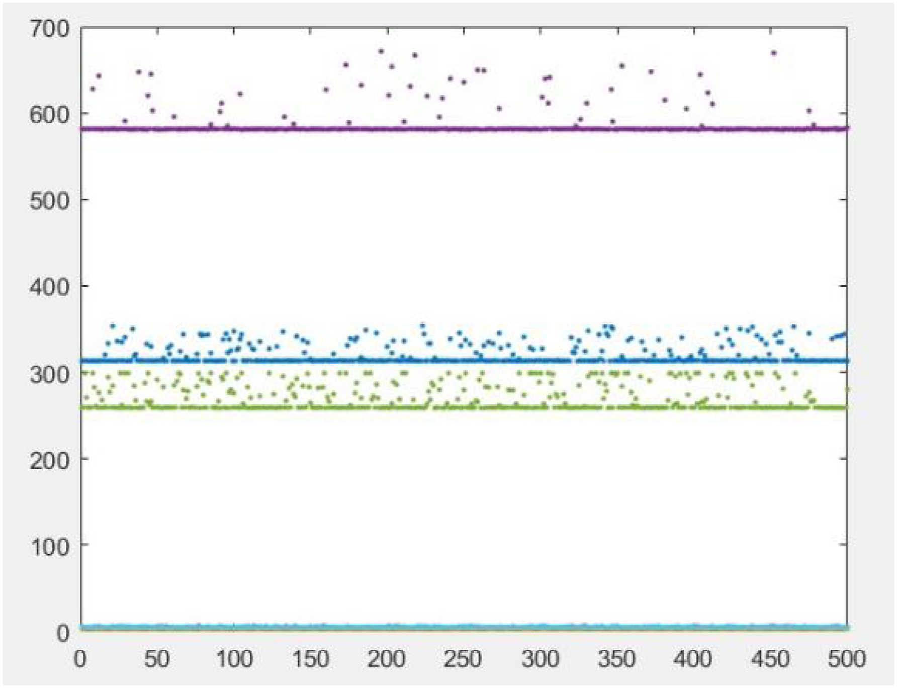
The iteration curve of the optimal solution of the PSO algorithm before modification is shown in Figure 13, and the distribution of it is shown in Figure 14. It can be seen that the optimized algorithm not only takes less time but also obtains a better optimal solution. The running time of the modified code is only 8.6 seconds. The iteration curve of its optimal solution is shown in Figure 15, and the distribution of particle swarm is shown in Figure 16. Iteration curve of the optimal solution before optimization. Distribution range of the particle swarm before optimization. Iteration curve of the optimal solution after optimization. Distribution range of the particle swarm after optimization.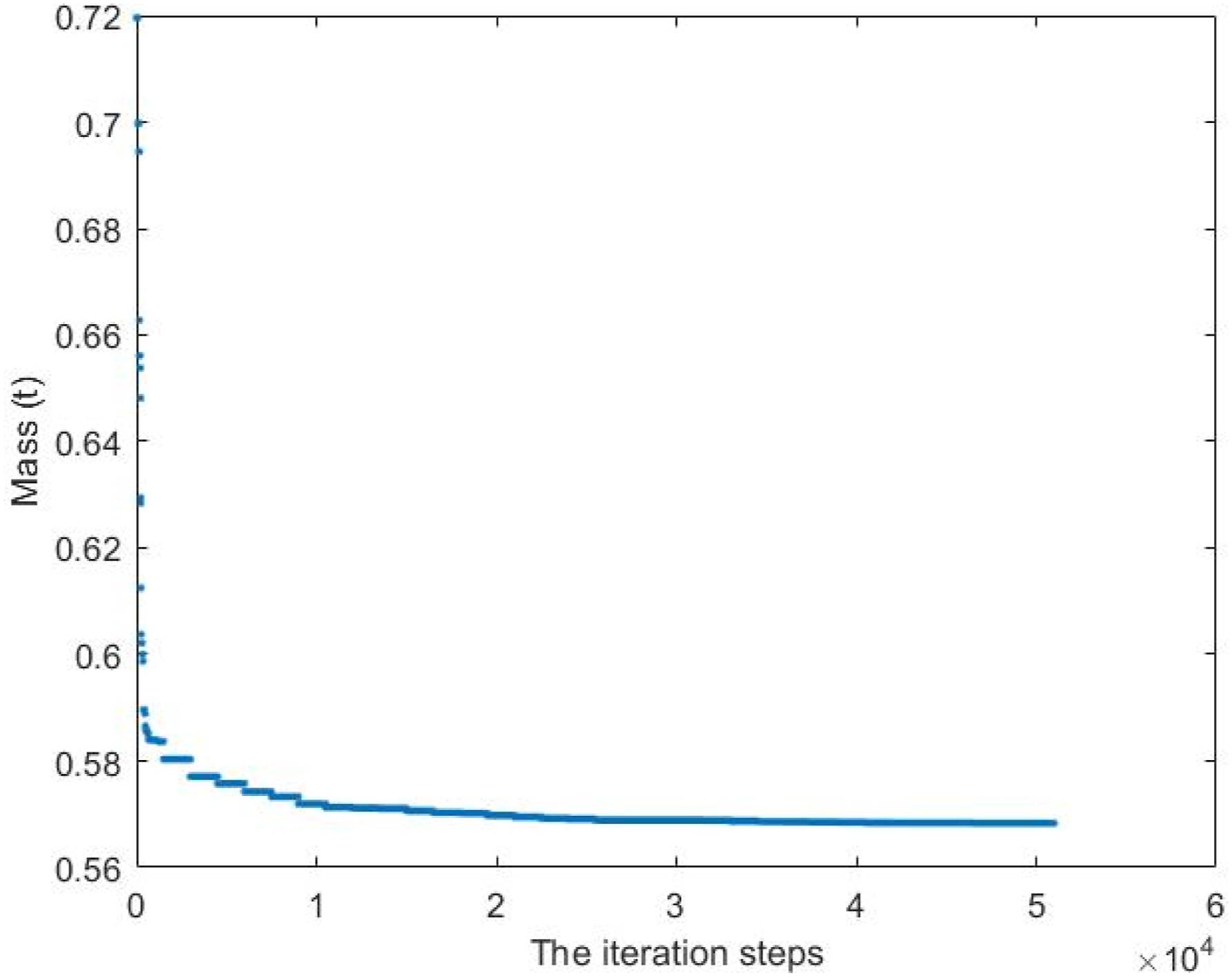
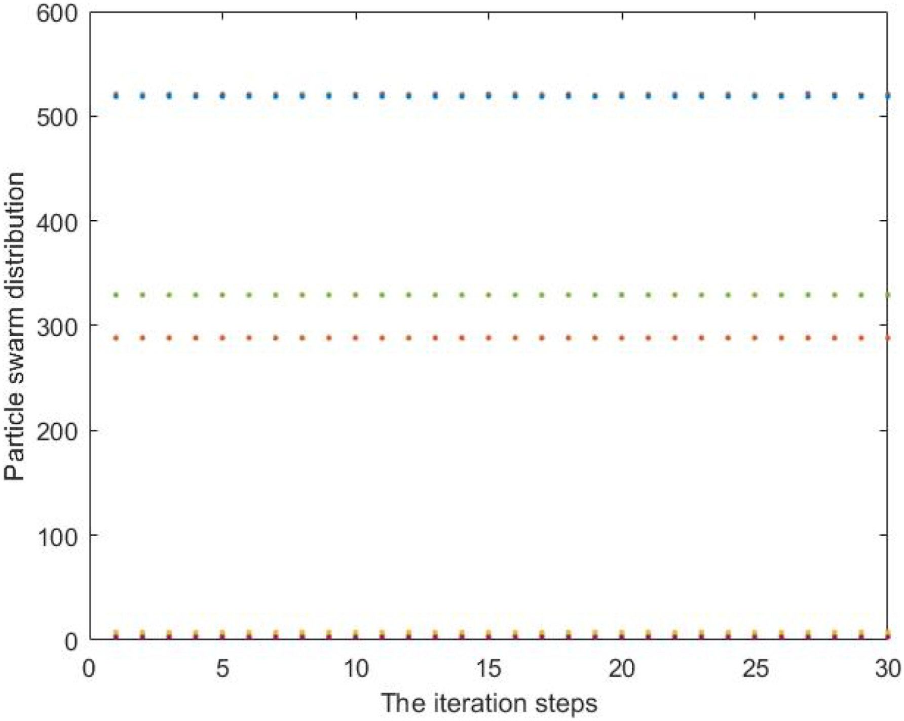
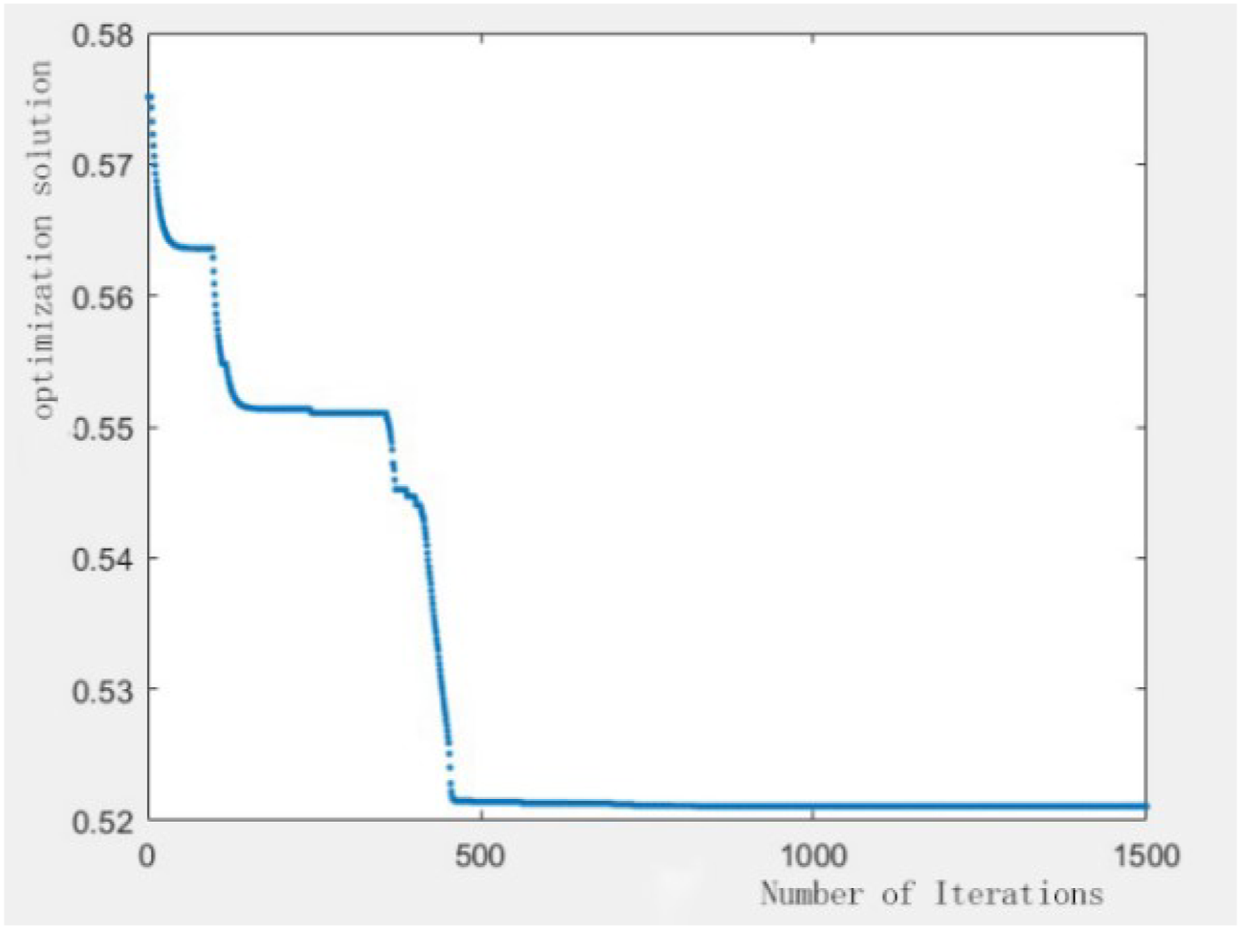
The original algorithm has fewer initial populations and low evolutionary generation, and mainly relies on repeated calculations for optimization. It has many iterations and long running time. The improved algorithm selects a large initial population and sets a larger number of evolutions. Particle swarm optimization has strong local optimization ability, fewer program iterations, shorter running time, and higher quality of the optimal solution.
The first step is to design the orthogonal test, and use the Workbench platform to calculate the simulation data under each case of the orthogonal test to obtain the simulation test data. The second step is to fit the data according to the results of the orthogonal test. The independent variables of the fitting function are six design variables, and the dependent variables of the fitting function are mass, natural frequency and maximum deformation. Three fitting functions are fitted respectively. The third step, the optimization objectives are determined, including six design variables and constraints, upon using the improved particle swarm optimization algorithm, after iterative optimization for getting the optimal solution under the improved particle swarm optimization, which are the optimized six independent variables, as shown in Figure17. Optimal solution of six independent variables after optimization.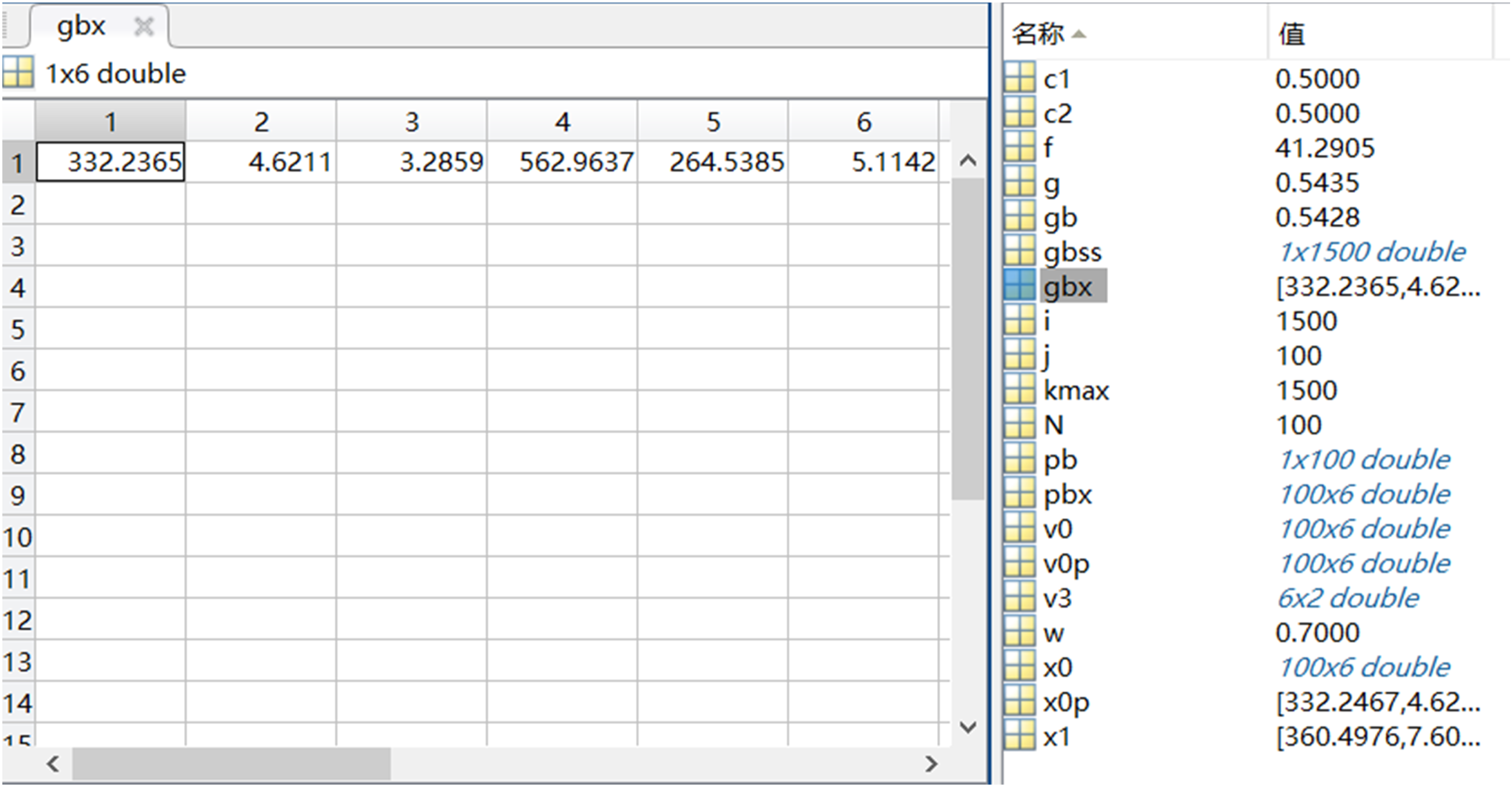
Parameters before and after optimization.
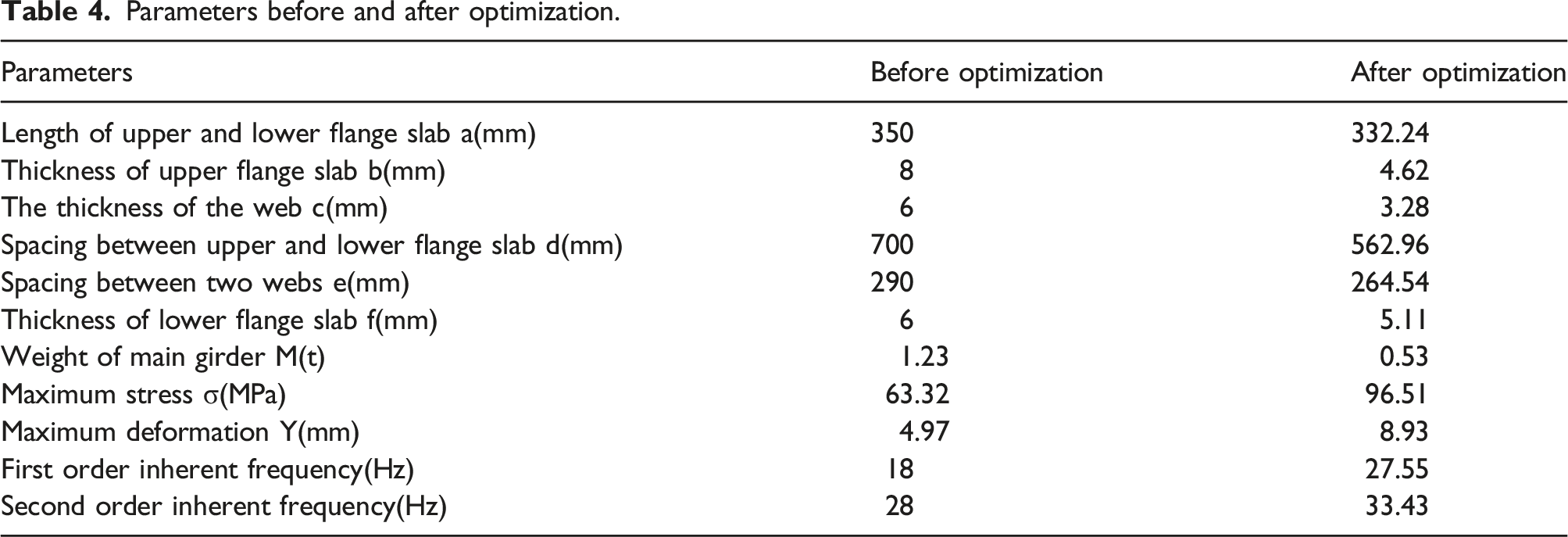
It can be seen from Table 4, the mass of the optimized main beam is 0.52 tons, which decreases by 58% compared with before optimization. Meanwhile, the maximum stress of the main beam increases to 96.78 MPa, and the maximum deformation of the main beam increases to 9 mm. The natural vibration frequency avoids the excitation frequency, and the structural redundancy is greatly reduced.
The model is carried out according to the optimized data, and the finite element analysis and modal analysis are conducted according to the above method. The maximum deformation results are shown in Figure 18; the maximum stress results are shown in Figure 19, and the modal analysis results are shown in Figure 20. Maximum deformation of the main beam after optimization. Maximum stress of the main beam after optimization. Mode of the main beam after optimization.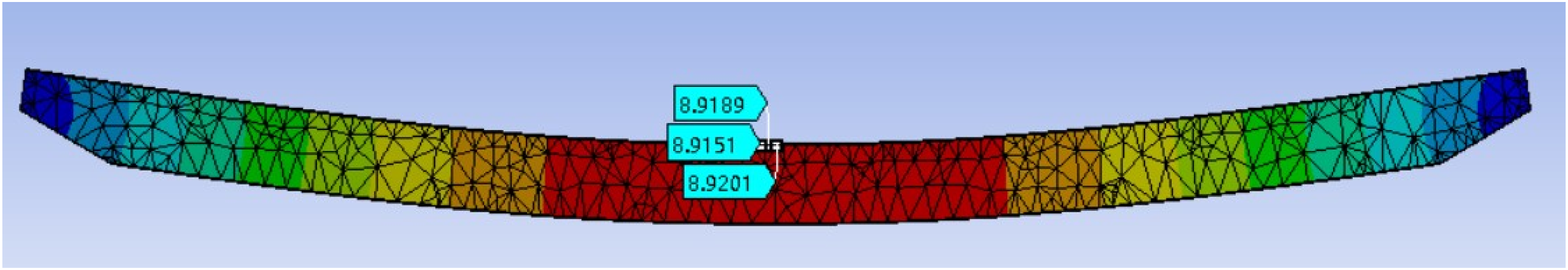
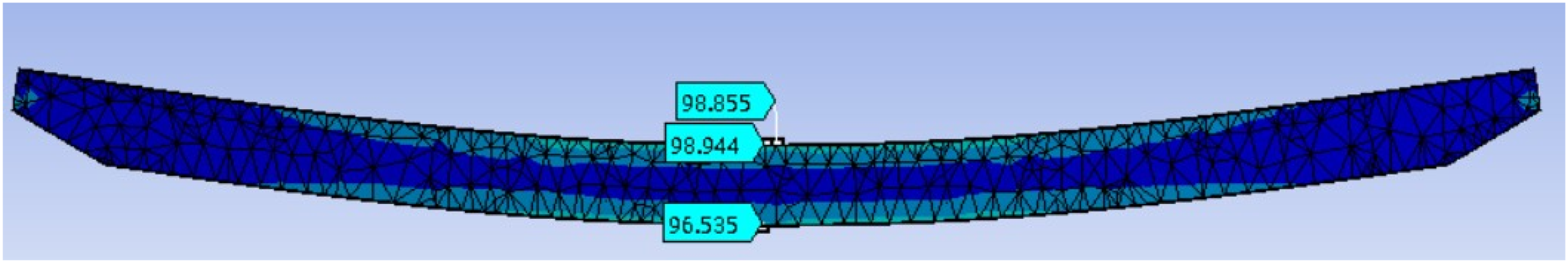
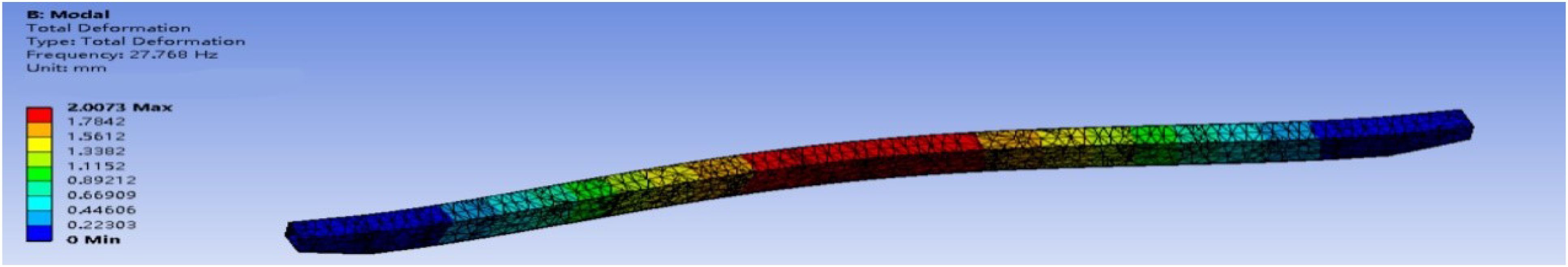
From Figure 18, Figure 19 and Figure 20, the maximum deformation and maximum stress of the optimized main beam are about 8.92 mm and 98.94 MPa, respectively. The solid vibration frequency is 27.77 Hz, which is not much different from the fitting calculation data. The accuracy of the previous optimization results is verified. At the same time, the vibration frequency of the main beam is higher than the excitation frequency of the motor, which can effectively avoid the resonance.
Conclusion
In this paper, in order to solve the problem of the large redundant coefficient of the main beam structure of the bridge crane, an orthogonal test table is designed. The required data are obtained by combining the calculation with finite element analysis, and the data are fitted. The functional relationship between the dependent and respective variables is obtained, and the optimization mathematical model is designed. Finally, the improved particle swarm algorithm is used to solve this model, and the optimal fitness value and a set of optimal independent variables are obtained. The analysis and solution results show that the maximum stress of the main beam increases from 63.32 MPa to 96.51 MPa, and the maximum deformation of the main beam increases from 4.97 mm to 8.93 mm. The first-order vibration frequency of the main beam increases from 18 Hz to 27.55 Hz, and the second-order vibration frequency of the main beam increases from 28 Hz to 33.43 Hz. The mass of the main beam decreases from 1.23 tons to 0.53 tons. The analysis and optimization results show that the quality, cost, and steel waste of the main beam are reduced largely when the parameters of the main beam meet the stability requirements.
Footnotes
Declaration of conflicting interests
The author(s) declared no potential conflicts of interest with respect to the research, authorship, and/or publication of this article.
Funding
The author(s) disclosed receipt of the following financial support for the research, authorship, and/or publication of this article: The project was supported by Henan Province Science and Technology Project (212102210051), Research on Key Technologies of Digital Design of High-speed Horizontal Machining Center.
Appendix
clear;
clc;
global c1 c2 wkmax N
c1=0.;
c2=0.5;
w=0.9;
kmax=1500;
N=500;
gbs=[];
v3=[300 400;3 10;3 10;400 900;240 350;3 10];
i=0;
while i<N
x1(1)=300+100*rand;
x1(2)=3+7*rand;
x1(3)=3+7*rand;
x1(4)=400+500*rand;
x1(5)=240+110*rand;
x1(6)=3+7*rand;
if0.2637*x1(1)+5.2318*x1(2)+5.8853*x1(3)+0.1762*x1(4)+0.0271*x1(5)+1.2212*x1(6)338.8933<0&&0.014*x1(1)
+0.1961*x1(2)+0.2994*x1(3)+0.0172*x1(4)+0.0074*x1(5)+0.3139*x1(6)-28.7872<0&&0.2637*x1(1)+5.2318
*x1(2)+5.8853*x1(3)+0.1762*x1(4)+0.0271*x1(5)+1.2212*x1(6)-338.8933<0&&0.014*x1(1)+0.1961*x1(2)
+0.2994*x1(3)+0.0172*x1(4)+0.0074*x1(5)+0.3139*x1(6)-28.7872<=0&&-0.2637*x1(1)-5.2318*x1(2)-5.8853*x1(3)-0.1762*x1(4)-0.0271*x1(5)-1.2212*x1(6)+338.8933-156<0&&-0.014*x1(1)-0.1961*x1(2)
0.2994*x1(3)-0.0172*x1(4)-0.0074*x1(5)-0.3139*x1(6)+28.7872-9<0 %Particles are generated under the conditions of stiffness and strength
i=i+1;
x0(i,1)=x1(1);
x0(i,2)=x1(2);
x0(i,3)=x1(3);
x0(i,4)=x1(4);
x0(i,5)=x1(5);
x0(i,6)=x1(6);
v0(i,1)=rand;
v0(i,2)=rand;
v0(i,3)=rand;
v0(i,4)=rand;
v0(i,5)=rand;
v0(i,6)=rand;
end
end
gbss=[];
pbx=x0;
gbx=x0(1,:);
gb=goal(gbx);
fori=1:N
pb(i)=goal(pbx(i,:)); if pb(i)<gb
gb=pb(i); gbx=pbx(i,:); end
end
fori=1:kmax
for j=1:N
v0p(j,:)=w*v0(j,:)+c1*rand*(pbx(j,:)-x0(j,:))+c2*rand*(gbx-x0(j,:)); %Update speed
v0p(j,:)=restrain(v0p(j,:),v3); %Limit the speed value to prevent excessive step size
x0p=x0(j,:)+v0p(j,:); %Update the individual
if fpen_in_fun1(x0p)
x0(j,:)=x0p; v0(j,:)=v0p(j,:);
end
g=goal(x0(j,:));
f=fn(x0(j,:));
if 0<f<14.4||17.6<f<18||22<f<22.5||27.5<f %Limited resonance interval
if g<pb(j)
pb(j)=g;
pbx(j,:)=x0(j,:);
if g<gb
gb=g;
gbx=x0(j,:);
end
end
end
end
gbss=[gbssgb];
end
plot(gbss,‘;.’)
x=gbx
result=gb
xlabel(‘Number of Iterations’)
ylabel(‘Optimization solution’)
plot(x0,‘.’)
function fc=fpen_in_fun1(x)
c=[ 0.2637*x(1)+5.2318*x(2)+5.8853*x(3)+0.1762*x(4)+0.0271*x(5)+1.2212*x(6)-338.8933
0.014*x(1)+0.1961*x(2)+0.2994*x(3)+0.0172*x(4)+0.0074*x(5)+0.3139*x(6)-28.7872
-0.2637*x(1)-5.2318*x(2)-5.8853*x(3)-0.1762*x(4)-0.0271*x(5)-1.2212*x(6)+182.8933
-0.014*x(1)-0.1961*x(2)-0.2994*x(3)-0.0172*x(4)-0.0074*x(5)-0.3139*x(6)+19.7872
x(1)-400
x(2)-10
x(3)-10
x(4)-900
x(5)-350
x(6)-10
-x(1)+300
-x(2)+3
-x(3)+3
-x(4)+400
-x(5)+240
-x(6)+3
];
ifisempty(find(c>=0)) %See if any of them are greater than or equal to 0
fc=1;
else
fc=0;
end
function f=goal(x) %Calculate the fitness value
f=0.0011*x(1)+0.0234*x(2)+0.0896*x(3)+0.000982*x(4)+0.0003994*x(5)+0.0214*x(6)-0.9931; end
function f=fn(x) %Calculate the frequency of solid vibration
f=0.013*x(1)-0.0467*x(2)+0.3905*x(3)+0.059*x(4)-0.0542*x(6)+2.9638; %Vibration model
end
function x=restrain(x1,xgate) %Put a speed limit on it
fori=1:length(x1)
x(i)=max(min((xgate(i,2)-xgate(i,1))/1000,x1(i)),-(xgate(i,2)-xgate(i,1))/1000);
end