Acoustic field characteristic analysis of the rotary acoustic cavity coupled system

Abstract

The rotary acoustic cavity coupled system can be generated in working conditions of aviation, aerospace, ship, machinery, and other fields. The rotary acoustic cavity includes cylindrical, spherical, and conical acoustic cavities, which integrates into the unified analysis model by iso-parametric transformation in finite element method. To study the acoustic field characteristic of rotary acoustic cavity coupled system, a unified analysis model of rotary acoustic cavity coupled system is established: First, the acoustic field characteristic of the coupled system is researched by improved Fourier series method, and the admissible sound pressure function is constructed by three-dimensional modified Fourier series. Then, the acoustic field domain energy functional is established, and the coupled domain energy functional including the coupled potential energy between the sound cavities is introduced to acquire the total energy functional of the coupled system. Finally, the energy equation is solved by Rayleigh–Ritz method, and the natural frequency and corresponding mode of the coupled system are obtained. The unified analysis model demonstrates excellent convergence and accuracy, which is verified by the results of finite element method. Sound pressure responses of the coupled system are obtained by introducing the internal point sound source excitation. The effect of relevant parameters of the coupled system on natural frequency and sound pressure response is investigated, which can provide theoretical guidance for vibration and noise reduction.

Introduction

The rotary cavity with arbitrary impedance wall is the basic structural element in aviation, aerospace, marine, and other fields. In addition to the single cavity structure, the cavity coupled system can also be generally used in actual engineering applications. Taking the aircraft as an instance, such as the cockpit and cabin, the complex space in the aircraft can be regarded as the irregular region formed by the coupling of several rotary cavities. The variation of sound pressure generated by excitation in the cockpit will change the sound pressure in the cabin, which in turn affects the sound pressure in the cockpit, forming a complex rotary acoustic cavity coupled system. To provide theoretical foundation for structural optimization and low noise design, it is indispensable to conduct intensive research on the unified analysis modeling of the rotary acoustic cavity coupled system which can reveal the acoustic field coupling mechanism.

In an idealized acoustic modeling, the acoustic walls of the cavity are assumed to be rigid walls, which provides a basis for the in-depth investigation of acoustic field characteristics. Compared with the acoustic cavity with rigid walls, the analytical model of dissipative walled acoustic cavity is closer to the practical engineering applications. In related studies, the acoustic analysis model of the rectangular acoustic cavity and prism acoustic cavity with dissipative acoustic walls have been researched by many scholars. Bistafa and Morrissey ¹ studied two numerical procedures to obtain the eigenvalues in the rectangular cavity with arbitrary wall impedances. Li and Cheng ² developed a fully coupled vibro-acoustic model to characterize the structural and acoustic coupling of a flexible panel backed by a rectangular-like cavity with a slight geometrical distortion, which is introduced through a tilted wall. By the Fourier series method, Du et al. ³ researched the acoustic analysis of a rectangular cavity with impedance boundary conditions arbitrarily specified on any of the walls, and present several numerical examples to demonstrate the effectiveness and reliability of the current method for various impedance boundary conditions. Zhao ⁴ developed a real-time algorithm for characterizing perforated liners damping at multiple mode frequencies, and comparison is made between the results from the algorithm and those from the short-time fast Fourier transform (FFT)–based techniques. Jin et al.^5,6 presented a general Chebyshev–Lagrangian method to obtain the analytical solution for a rectangular acoustic cavity with arbitrary impedance walls. The interior two-dimensional acoustic modeling and modal analysis are presented in the framework of iso geometric analysis (IGA). Bilbao et al. ⁷ incorporated general locally reactive impedance boundary conditions into a 3D finite volume time domain formulation, which may be specialized to the various types of finite difference time domain method under fitted boundary termination. Shi et al. ⁸ proposed a method for the analysis of acoustic modals and steady-state responses of arbitrary triangular prism and quadrangular prism acoustic cavities with impedance walls based on the three-dimensional improved Fourier series. Within the framework of Hamilton’s principle, Shao et al. ⁹ established a simple and unified process for transient vibration analysis of functionally graded material (FGM) sandwich plates in thermal environment.

Numerous models of the rotary acoustic cavity are applied to analyze many practical engineering environments. Therefore, an increasing number of researchers have concentrated on the investigation of the rotary acoustic cavity analysis model. From classical linearized acoustics, Rona ¹⁰ conducted on the acoustic resonance that develops in rectangular and cylindrical cavities, and an analytical model for the small amplitude acoustic perturbations inside an enclosure with rigid walls is constructed. Bennett ¹¹ investigated the interaction between the shear layer over a circular cavity and the flow-excited acoustic response of the volume to shear layer instability modes. Jeong et al. ¹² presented an analytical model for acoustic transmission characteristics of a cylindrical cavity system with radiation impedance walls representing the acoustic resonance conditions of a Korean bell. Through simulation and experimental studies, Blimbaum et al. ¹³ have analyzed the multi-dimensional acoustic field excited by transverse acoustic disturbances interacting with an annular side branch to emulate a fuel/air mixing nozzle. Lee ¹⁴ presented a semi-analytical approach to solve the eigenproblem of a 2D acoustic cavity with multiple elliptical boundaries, and then he ¹⁵ solved acoustic eigenproblems of 3D elliptical cylindrical cavities having multiple elliptical cylinders by means of a 3D semi-analytical formulation based on a multipole expansion. Chen et al. ¹⁶ investigated the structural–acoustic radiation problem of cylindrical shell structures with complex acoustic boundary conditions. The structural–acoustic radiation problem of a cylindrical shell is solved by using the double reflection method. Li et al. ¹⁷ derived the analytical solutions of the acoustic field in annular combustion chambers with both varying cross-sectional surface area and average radius sustaining a mean flow. Shao et al. ¹⁸ investigated the damping performances of seven single- and one double-layer perforated liners with different open area ratios experimentally. Meanwhile, a cold-flow pipe with a lined section is designed. It can be found from the existing literature that studies about analysis model of the rotary acoustic cavity coupled system which have been attempted are concentrated on the cylindrical cavity, while spherical and conical acoustic cavities are seldom involved. Particularly, there are few investigations of the unified analysis model of rotary acoustic cavity.

In many engineering practices, a single cavity structure cannot represent an integrated complex engineering structure such as aircraft and submarine. Hence the acoustic cavity coupled system has come into the field of scholars. Lee ¹⁹ proposed an advanced analytical method that can be applied to obtain acoustical modal properties of multiple three-dimensional (3D) rectangular cavities and the modal properties of a 3D coupled structural–acoustic system including the multiple cavities, where cavities are connected in series by necks. Unnikrishnan et al. ²⁰ presented a simplified modeling approach for numerical simulation of a coupled cavity–resonator system which is validated by experiments. Tanaka et al. ²¹ derived explicitly the eigenpairs of a coupled rectangular cavity comprising five rigid walls and one flexible panel, which are yet to be found in much literature. Birk et al. ²² presented a high-order doubly asymptotic open boundary for modeling scalar wave propagation in two-dimensional unbounded media. By using a circular boundary to divide these into near field and far field, the present method is capable of handling domains with arbitrary geometry. Using the Lagrange multiplier technique, Chen et al. ²³ proposed a domain decomposition method to predict the acoustic characteristics of an arbitrary enclosure made up of any number of sub-spaces, which avoided involving extra coupling parameters and theoretically ensures the continuity conditions of both sound pressure and particle velocity at the coupling interface. Shi et al. ²⁴ concerned with the modeling and acoustic eigenanalysis of coupled rectangular spaces with a coupling aperture of variable size. Based on the energy principle, a modeling method for this problem is developed in combination with a 3D modified Fourier cosine series approach. Moores et al. ²⁵ demonstrated an acoustical analog of a circuit quantum electrodynamics system that leverages acoustic properties to enable strong multimode coupling in the dispersive regime while suppressing spontaneous emission to unconfined modes. Although many investigations of acoustic cavity coupled system have been conducted, the shape of acoustic cavities in coupled system is mainly rectangular, while the rotary acoustic cavity coupled system is rarely involved. Meanwhile, sectional literature purely refers to the analysis of the coupling mechanism between acoustic cavities, but do not specifically establish a unified analysis model, especially a unified analysis model of the rotary acoustic cavity coupled system.

Contrapose the shortcomings of the existing studies, a unified analysis model of the rotary acoustic cavity coupled system is established in this paper, and its acoustic field characteristics are analyzed. First, the expression of the admissible sound pressure functions in the coupled system is constructed. Second, the energy functional of acoustic field is established, and the coupling potential energy between acoustic cavities is added to obtain the energy functional of the whole coupled system. Then, the solution equation of acoustic field coupling mechanism in the coupled system is acquired by Rayleigh–Ritz method, and the acoustic field characteristics of the system can be obtained by solving the equation. Finally, based on the verification of the fast convergence and accuracy of the model, the effect of relevant parameters on the acoustic field characteristics is analyzed, and the point acoustic source excitation is introduced to research the acoustic pressure response of the coupled system.

Unified analysis modeling process

Model description

Rotary cylindrical, spherical, and conical acoustic cavities can be represented by the special cases of double curvature cavity elements. It is demonstrated in Figure 1 that an orthogonal coordinate system is established with the base plane of the element (z = 0) as the reference plane. R _α and R _β denote the reference radius of curvature along the α axis and β axis. L _α and L _β represent length dimensions along the α axis and β axis, and L _z represents the height dimensions along the z axis of the acoustic cavity.

Figure 1.

Cross-section geometrical parameters and coordinate system of double curvature cavity element.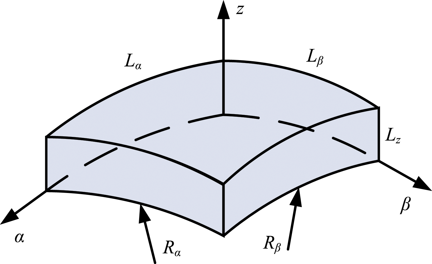

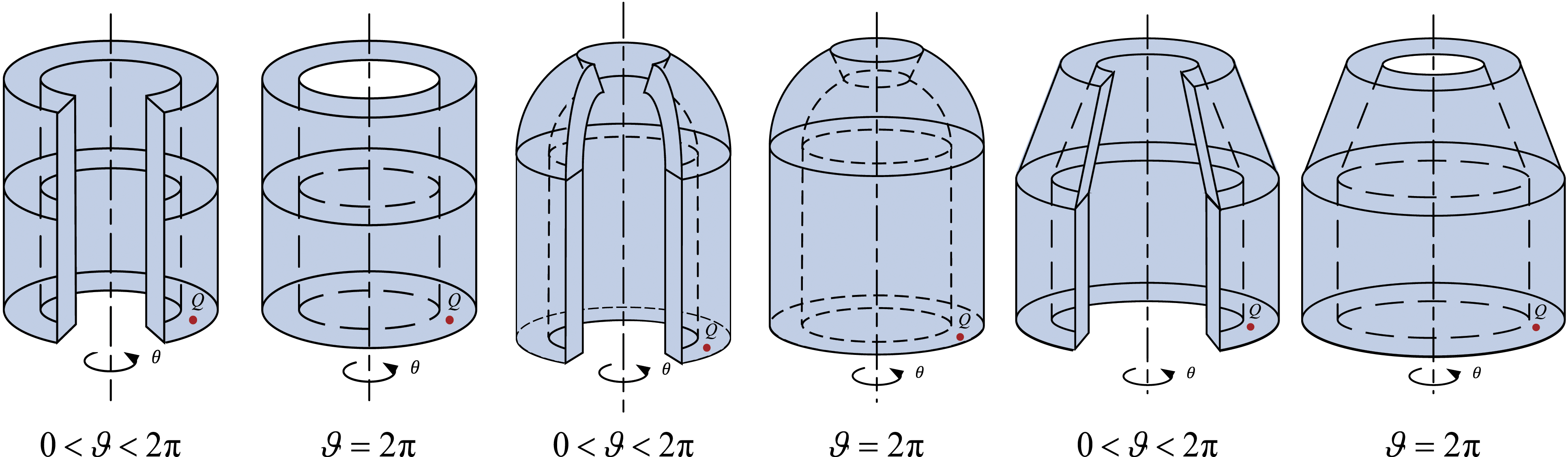
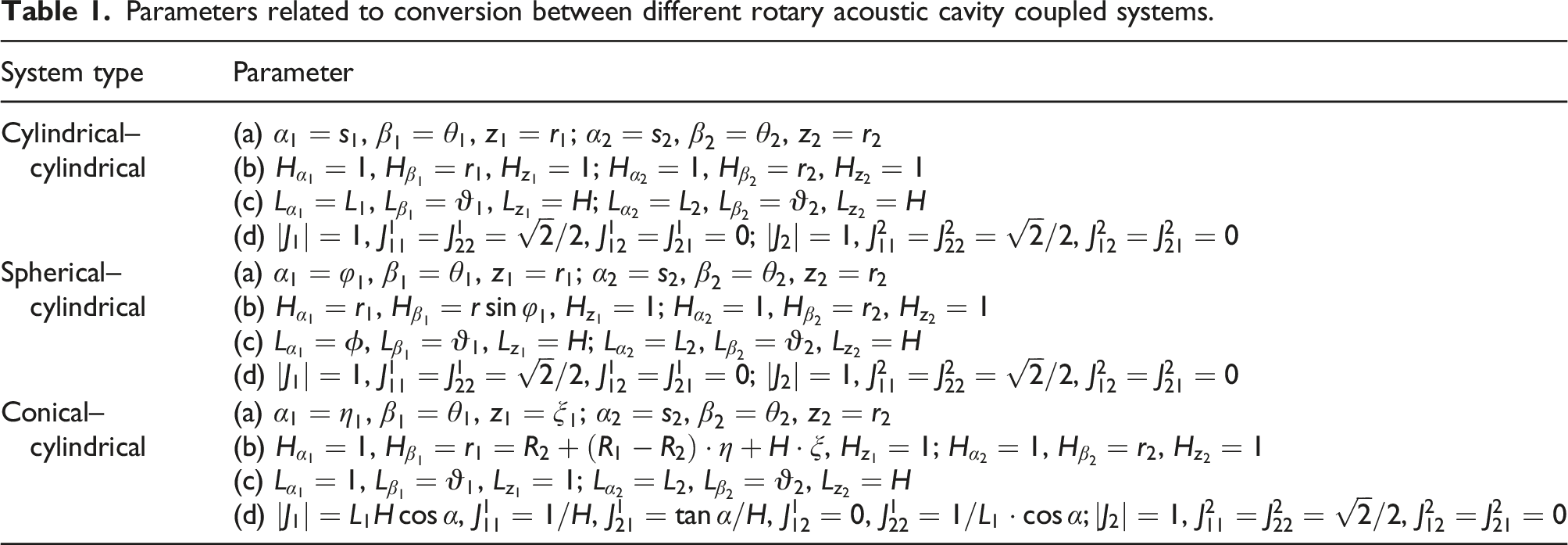
Figure 2 demonstrates the cross-section geometrical parameters and coordinate system of rotary acoustic cavity coupled systems: (a) The cylindrical–cylindrical acoustic cavity coupled system consists of two local coordinate systems (o-s₁, θ₁, r₁) and (o-s₂, θ₂, r₂). The inner radius and outer radius of cylindrical cavities are denoted by R₁ and R₂, the thickness is represented by H, and the height of two cavities is marked as L₁ and L₂, respectively. (b) The spherical–cylindrical acoustic cavity coupled system consists of two local coordinate systems (o-φ₁, θ₁, r₁) and (o-s₂, θ₂, r₂). R₁ and R₂ separately represent the inner radius and outer radius of spherical cavity and cylindrical cavity, and H is their thickness. The apex angle of spherical cavity can be represented by ϕ, where ϕ = ϕ₂ − ϕ₁. The height of cylindrical cavity is denoted by L. (c) The conical–cylindrical acoustic cavity coupled system consists of two local coordinate systems (o-s₁, θ₁, r₁) and (o-s₂, θ₂, r₂). R₁ and R₂ are the short radius and long radius of conical cavity, α and L₁ are the cone–apex angle and the length of generatrix of conical cavity. The inner radius and outer radius of cylindrical cavity are denoted by R₂ and R₃, and the height is denoted by L₂. H is the thickness of the whole coupled system. Figure 3 shows the shapes of rotary acoustic cavity coupled system at different rotation angles, in which ϑ is the rotation angle of the coupled system. When ϑ = 2π, the coupled systems have two walls coupling which causes the reduction of two walls. To investigate the acoustic response characteristics, a monopole point acoustic source Q is placed in the coupled system.

Figure 2.

Cross-section geometrical parameters and coordinate system of the rotary acoustic cavity coupled system. (a) Cylindrical–cylindrical acoustic cavity coupled system (b) Spherical–cylindrical acoustic cavity coupled system (c) Conical–cylindrical acoustic cavity coupled system.

Figure 3.

Unified model of the rotary acoustic cavity coupled system.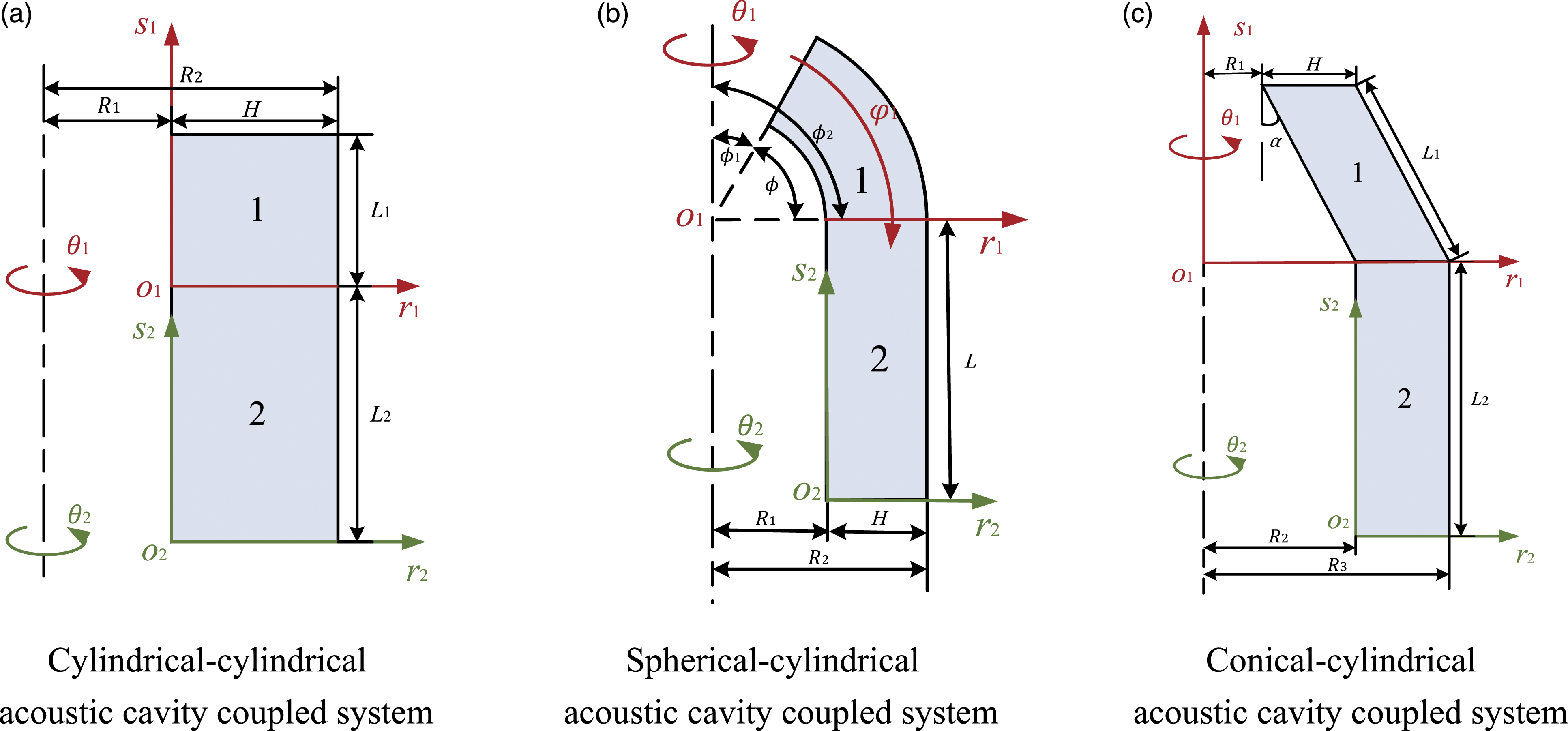

Related parameters

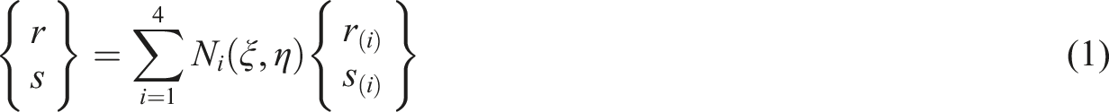
To establish the coupling mechanism between two acoustic cavities, the parallelogram section in rotary acoustic cavity coupled system is necessary to be transformed into a square section. As is shown in Figure 4, the plane ξoη coordinate system is transformed from plane ros coordinate system by iso-parametric transformation.

Figure 4.

Schematic diagram of coordinate transformation of parallelogram section.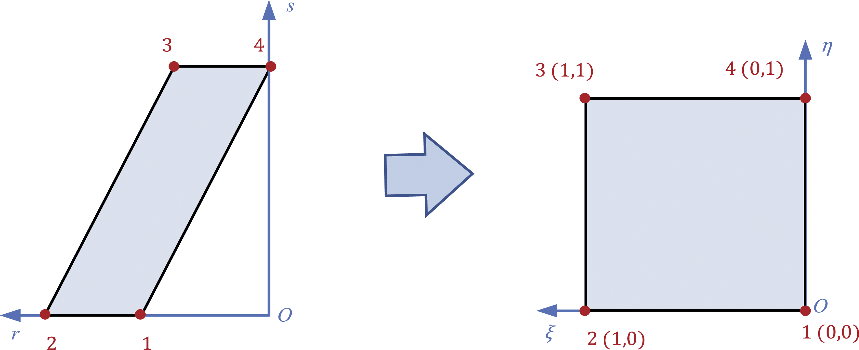

The coordinate transformation equation and the shape function expression are shown in equations (1) and (2)

$$\left\{\begin{array}{l}r\\ s\end{array}\right\}={\displaystyle \sum _{i=1}^4{N}_i\left(\xi ,\eta \right)}\left\{\begin{array}{l}{r}_{\left(i\right)}\\ s_{\left(i\right)}\end{array}\right\}$$

(1)

$$N_i\left(\xi ,\eta \right)={\left(-1\right)}^{i+1}\left(1-{\xi }_{\left(i\right)}-\xi \right)\left(1-{\eta }_{\left(i\right)}-\eta \right)$$

(2)

where (r_(i), s_(i)) and (ξ_(i), η_(i)) are separately the coordinate of the i ^th vertex of the plane ros coordinate system and plane ξoη coordinate system, N _i (ξ, η) represents the shape function of the i ^th vertex of the plane ros coordinate system.

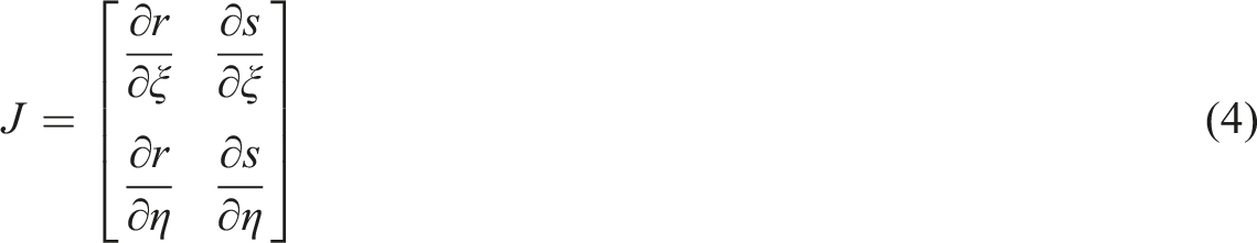
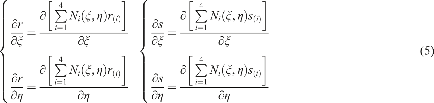
The transformation of coordinates is written in matrix form equations (3) and (4)

$${\left[\begin{array}{cc}\frac{\partial }{\partial \xi }& \frac{\partial }{\partial \eta }\end{array}\right]}^{\mathrm{T}}=J{\left[\begin{array}{cc}\frac{\partial }{\partial r}& \frac{\partial }{\partial s}\end{array}\right]}^{\mathrm{T}}$$

(3)

$$J=\left[\begin{array}{cc}\frac{\partial r}{\partial \xi }& \frac{\partial s}{\partial \xi }\\ \frac{\partial r}{\partial \eta }& \frac{\partial s}{\partial \eta }\end{array}\right]$$

(4)

in which $\frac{\partial r}{\partial \xi }$ , $\frac{\partial r}{\partial \eta }$ , $\frac{\partial s}{\partial \xi }$ and $\frac{\partial s}{\partial \eta }$ can be denoted by equation (5)

$$\{\begin{array}{l}\frac{\partial r}{\partial \xi }=\frac{\partial \left[{\displaystyle \sum _{i=1}^4{N}_i\left(\xi ,\eta \right)r_{\left(i\right)}}\right]}{\partial \xi }\\ \frac{\partial r}{\partial \eta }=\frac{\partial \left[{\displaystyle \sum _{i=1}^4{N}_i\left(\xi ,\eta \right)r_{\left(i\right)}}\right]}{\partial \eta }\end{array}\hspace{0.17em}\hspace{0.17em}\hspace{0.17em}\hspace{0.17em}\{\begin{array}{l}\frac{\partial s}{\partial \xi }=\frac{\partial \left[{\displaystyle \sum _{i=1}^4{N}_i\left(\xi ,\eta \right)s_{\left(i\right)}}\right]}{\partial \xi }\\ \frac{\partial s}{\partial \eta }=\frac{\partial \left[{\displaystyle \sum _{i=1}^4{N}_i\left(\xi ,\eta \right)s_{\left(i\right)}}\right]}{\partial \eta }\end{array}$$

(5)

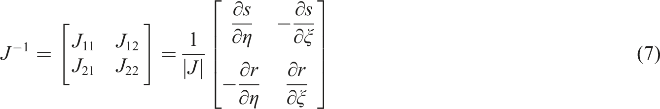
Equation (3) can also be expressed in the inverse form

$${\left[\begin{array}{cc}\frac{\partial }{\partial r}& \frac{\partial }{\partial s}\end{array}\right]}^{\mathrm{T}}=J^{-1}{\left[\begin{array}{cc}\frac{\partial }{\partial \xi }& \frac{\partial }{\partial \eta }\end{array}\right]}^{\mathrm{T}}$$

(6)

$$J^{-1}=\left[\begin{array}{cc}{J}_{11}& J_{12}\\ J_{21}& J_{22}\end{array}\right]=\frac{1}{\left|J\right|}\left[\begin{array}{cc}\frac{\partial s}{\partial \eta }& -\frac{\partial s}{\partial \xi }\\ -\frac{\partial r}{\partial \eta }& \frac{\partial r}{\partial \xi }\end{array}\right]$$

(7)

where $\left|J\right|$ is the determinant of the Jacobian matrix.

Table 1 shows the parameters referential to conversion between different rotary acoustic cavity coupled systems: (a) The relation between the local coordinate system and the coordinate system of double curvature cavity element; (b) the Lame coefficient; (c) the maximum value of each coordinate axis; (d) coordinate transformation parameter.

Table 1.

Parameters related to conversion between different rotary acoustic cavity coupled systems.

System type	Parameter
Cylindrical–cylindrical	(a) ${\alpha }_1=s_1,{\beta }_1={\theta }_1,z_1=r_1;{\alpha }_2=s_2,{\beta }_2={\theta }_2,z_2=r_2$
	(b) $H_{{\alpha }_1}=1,H_{{\beta }_1}=r_1,H_{z_1}=1;H_{{\alpha }_2}=1,H_{{\beta }_2}=r_2,H_{z_2}=1$
	(c) $L_{{\alpha }_1}=L_1,L_{{\beta }_1}={\vartheta }_1,L_{z_1}=H;L_{{\alpha }_2}=L_2,L_{{\beta }_2}={\vartheta }_2,L_{z_2}=H$
	(d) $\left|J_1\right|=1,J_{11}^1=J_{22}^1=\sqrt{2}/2,J_{12}^1=J_{21}^1=0;\left|J_2\right|=1,J_{11}^2=J_{22}^2=\sqrt{2}/2,J_{12}^2=J_{21}^2=0$
Spherical–cylindrical	(a) ${\alpha }_1={\phi }_1,{\beta }_1={\theta }_1,z_1=r_1;{\alpha }_2=s_2,{\beta }_2={\theta }_2,z_2=r_2$
	(b) $H_{{\alpha }_1}=r_1,H_{{\beta }_1}=r\sin {\phi }_1,H_{z_1}=1;H_{{\alpha }_2}=1,H_{{\beta }_2}=r_2,H_{z_2}=1$
	(c) $L_{{\alpha }_1}=\varphi ,L_{{\beta }_1}={\vartheta }_1,L_{z_1}=H;L_{{\alpha }_2}=L_2,L_{{\beta }_2}={\vartheta }_2,L_{z_2}=H$
	(d) $\left|J_1\right|=1,J_{11}^1=J_{22}^1=\sqrt{2}/2,J_{12}^1=J_{21}^1=0;\left|J_2\right|=1,J_{11}^2=J_{22}^2=\sqrt{2}/2,J_{12}^2=J_{21}^2=0$
Conical–cylindrical	(a) ${\alpha }_1={\eta }_1,{\beta }_1={\theta }_1,z_1={\xi }_1;{\alpha }_2=s_2,{\beta }_2={\theta }_2,z_2=r_2$
	(b) $H_{{\alpha }_1}=1,H_{{\beta }_1}=r_1=R_2+\left(R_1-R_2\right)\cdot \eta +H\cdot \xi ,H_{z_1}=1;H_{{\alpha }_2}=1,H_{{\beta }_2}=r_2,H_{z_2}=1$
	(c) $L_{{\alpha }_1}=1,L_{{\beta }_1}={\vartheta }_1,L_{z_1}=1;L_{{\alpha }_2}=L_2,L_{{\beta }_2}={\vartheta }_2,L_{z_2}=H$
	(d) $\left|J_1\right|=L_{1}H\cos \alpha ,J_{11}^1=1/H,J_{21}^1=\tan \alpha /H,J_{12}^1=0,J_{22}^1=1/L_1\cdot \cos \alpha ;\left|J_2\right|=1,J_{11}^2=J_{22}^2=\sqrt{2}/2,J_{12}^2=J_{21}^2=0$

Construction of admissible sound pressure functions

The rotary acoustic cavity coupled system can be divided into two sound field domains and the coupling domain represented by the contact surfaces of two enclosed acoustic cavities, hence two sound pressure admissible functions are established, respectively. The expression of the admissible sound pressure function expressed by three-dimensional modified Fourier series method is the superposition of one multiplied cosine function and six multiplied sines and cosines

$$P_n\left({\alpha }_n,{\beta }_n,z_n\right)=P_n^{\mathrm{\Omega }}\left({\alpha }_n,{\beta }_n,z_n\right)+{\displaystyle \sum _{q=1}^6{P}_n^{{\mathrm{\Theta }}_q}\left({\alpha }_n,{\beta }_n,z_n\right)}$$

(8)

in which n is introduced here to represent the sequence number of acoustic cavities in the coupled system. The expression of sound pressure inside the n ^th cavity of the coupled system is denoted by $P_{\mathrm{\Omega }}^n\left({\alpha }_n,{\beta }_n,z_n\right)$ , and $P_{{\mathrm{\Theta }}_q}^n\left({\alpha }_n,{\beta }_n,z_n\right)$ is the q ^th supplementary polynomial of the n ^th cavity. The specific expressions are demonstrated as equations. (9)–(12)

$$P_1^{\mathrm{\Omega }}\left({\alpha }_1,{\beta }_1,z_1\right)={\displaystyle \sum _{m=0}^{+\infty }{\displaystyle \sum _{n=0}^{+\infty }{\displaystyle \sum _{l=0}^{+\infty }{G}_{mnl}^1\cos \left({\lambda }_{{\alpha }_1}{\alpha }_1\right)}\cos \left({\lambda }_{{\beta }_1}{\beta }_1\right)}}\cos \left({\lambda }_{z_1}{z}_1\right)$$

(9)

$$P_1^{{\mathrm{\Theta }}_1}\left({\alpha }_1,{\beta }_1,z_1\right)={\displaystyle \sum _{m=-2}^{-1}{\displaystyle \sum _{n=0}^{+\infty }{\displaystyle \sum _{l=0}^{+\infty }{G}_{mnl}^2\sin \left({\lambda }_{{\alpha }_1}{\alpha }_1\right)}}\cos \left({\lambda }_{{\beta }_1}{\beta }_1\right)}\cos \left({\lambda }_{z_1}{z}_1\right)$$

(10a)

$$P_1^{{\mathrm{\Theta }}_2}\left({\alpha }_1,{\beta }_1,z_1\right)={\displaystyle \sum _{m=0}^{+\infty }{\displaystyle \sum _{n=-2}^{-1}{\displaystyle \sum _{l=0}^{+\infty }{G}_{mnl}^3\cos \left({\lambda }_{{\alpha }_1}{\alpha }_1\right)}\sin \left({\lambda }_{{\beta }_1}{\beta }_1\right)}}\cos \left({\lambda }_{z_1}{z}_1\right)$$

(10b)

$$P_1^{{\mathrm{\Theta }}_3}\left({\alpha }_1,{\beta }_1,z_1\right)={\displaystyle \sum _{m=0}^{+\infty }{\displaystyle \sum _{n=0}^{+\infty }{\displaystyle \sum _{l=-2}^{-1}{G}_{mnl}^4\cos \left({\lambda }_{{\alpha }_1}{\alpha }_1\right)}\cos \left({\lambda }_{{\beta }_1}{\beta }_1\right)}}\sin \left({\lambda }_{z_1}{z}_1\right)$$

(10c)

$$P_1^{{\mathrm{\Theta }}_4}\left({\alpha }_1,{\beta }_1,z_1\right)={\displaystyle \sum _{m=-2}^{-1}{\displaystyle \sum _{n=-2}^{-1}{\displaystyle \sum _{l=0}^{+\infty }{G}_{mnl}^5\sin \left({\lambda }_{{\alpha }_1}{\alpha }_1\right)}}}\sin \left({\lambda }_{{\beta }_1}{\beta }_1\right)\cos \left({\lambda }_{z_1}{z}_1\right)$$

(10d)

$$P_1^{{\mathrm{\Theta }}_5}\left({\alpha }_1,{\beta }_1,z_1\right)={\displaystyle \sum _{m=-2}^{-1}{\displaystyle \sum _{n=0}^{+\infty }{\displaystyle \sum _{l=-2}^{-1}{G}_{mnl}^6\sin \left({\lambda }_{{\alpha }_1}{\alpha }_1\right)}\cos \left({\lambda }_{{\beta }_1}{\beta }_1\right)}}\sin \left({\lambda }_{z_1}{z}_1\right)$$

(10e)

$$P_1^{{\mathrm{\Theta }}_6}\left({\alpha }_1,{\beta }_1,z_1\right)={\displaystyle \sum _{m=0}^{+\infty }{\displaystyle \sum _{n=-2}^{-1}{\displaystyle \sum _{l=-2}^{-1}{G}_{mnl}^6\cos \left({\lambda }_{{\alpha }_1}{\alpha }_1\right)}\sin \left({\lambda }_{{\beta }_1}{\beta }_1\right)}}\sin \left({\lambda }_{z_1}{z}_1\right)$$

(10f)

$$P_2^{\mathrm{\Omega }}\left({\alpha }_2,{\beta }_2,z_2\right)={\displaystyle \sum _{m=0}^{+\infty }{\displaystyle \sum _{n=0}^{+\infty }{\displaystyle \sum _{l=0}^{+\infty }{H}_{mnl}^1\cos \left({\lambda }_{{\alpha }_2}{\alpha }_2\right)}\cos \left({\lambda }_{{\beta }_2}{\beta }_2\right)}}\cos \left({\lambda }_{z_2}{z}_2\right)$$

(11)

$$P_2^{{\mathrm{\Theta }}_1}\left({\alpha }_2,{\beta }_2,z_2\right)={\displaystyle \sum _{m=-2}^{-1}{\displaystyle \sum _{n=0}^{+\infty }{\displaystyle \sum _{l=0}^{+\infty }{H}_{mnl}^2\sin \left({\lambda }_{{\alpha }_2}{\alpha }_2\right)}\cos \left({\lambda }_{{\beta }_2}{\beta }_2\right)}}\cos \left({\lambda }_{z_2}{z}_2\right)$$

(12a)

$$P_2^{{\mathrm{\Theta }}_2}\left({\alpha }_2,{\beta }_2,z_2\right)={\displaystyle \sum _{m=0}^{+\infty }{\displaystyle \sum _{n=-2}^{-1}{\displaystyle \sum _{l=0}^{+\infty }{H}_{mnl}^3\cos \left({\lambda }_{{\alpha }_2}{\alpha }_2\right)}\sin \left({\lambda }_{{\beta }_2}{\beta }_2\right)}}\cos \left({\lambda }_{z_2}{z}_2\right)$$

(12b)

$$P_2^{{\mathrm{\Theta }}_3}\left({\alpha }_2,{\beta }_2,z_2\right)={\displaystyle \sum _{m=0}^{+\infty }{\displaystyle \sum _{n=0}^{+\infty }{\displaystyle \sum _{l=-2}^{-1}{H}_{mnl}^4\cos \left({\lambda }_{{\alpha }_2}{\alpha }_2\right)}\cos \left({\lambda }_{{\beta }_2}{\beta }_2\right)}}\sin \left({\lambda }_{z_2}{z}_2\right)$$

(12c)

$$P_2^{{\mathrm{\Theta }}_4}\left({\alpha }_2,{\beta }_2,z_2\right)={\displaystyle \sum _{m=-2}^{-1}{\displaystyle \sum _{n=-2}^{-1}{\displaystyle \sum _{l=0}^{+\infty }{H}_{mnl}^5\sin \left({\lambda }_{{\alpha }_2}{\alpha }_2\right)}\sin \left({\lambda }_{{\beta }_2}{\beta }_2\right)}}\cos \left({\lambda }_{z_2}{z}_2\right)$$

(12d)

$$P_2^{{\mathrm{\Theta }}_5}\left({\alpha }_2,{\beta }_2,z_2\right)={\displaystyle \sum _{m=-2}^{-1}{\displaystyle \sum _{n=0}^{+\infty }{\displaystyle \sum _{l=-2}^{-1}{H}_{mnl}^6\sin \left({\lambda }_{{\alpha }_2}{\alpha }_2\right)}\cos \left({\lambda }_{{\beta }_2}{\beta }_2\right)}}\sin \left({\lambda }_{z_2}{z}_2\right)$$

(12e)

$$P_2^{{\mathrm{\Theta }}_6}\left({\alpha }_2,{\beta }_2,z_2\right)={\displaystyle \sum _{m=0}^{+\infty }{\displaystyle \sum _{n=-2}^{-1}{\displaystyle \sum _{l=-2}^{-1}{H}_{mnl}^7\cos \left({\lambda }_{{\alpha }_2}{\alpha }_2\right)}\sin \left({\lambda }_{{\beta }_2}{\beta }_2\right)}}\sin \left({\lambda }_{z_2}{z}_2\right)$$

(12f)

where ${\lambda }_{{\alpha }_1}=m\pi /L_{{\alpha }_1},{\lambda }_{{\alpha }_2}=m\pi /L_{{\alpha }_2},{\lambda }_{{\beta }_1}=m\pi /L_{{\beta }_1},{\lambda }_{{\beta }_2}=m\pi /L_{{\beta }_2},{\lambda }_{z_1}=m\pi /L_{z_1},{\lambda }_{z_2}=m\pi /L_{z_2}$ , $G_{mnl}^t$ and $H_{mnl}^t$ are three-dimensional unknown Fourier coefficients of two admissible sound pressure functions. All of them will be determined by the Rayleigh–Ritz procedure.

Energy equation

Rayleigh–Ritz energy method is applied to research the acoustic field characteristic. The Lagrange equation of the established acoustic cavity coupled system model can be written as

$$L_{C_1}=U_{C_1}-T_{C_1}-W_{\mathrm{wall}}^1+W_{\mathrm{coupling}}^1-W_{\mathrm{sound}}^1-W_{C_1-C_2}$$

(13)

$$L_{C_2}=U_{C_2}-T_{C_2}-W_{\mathrm{wall}}^2+W_{\mathrm{coupling}}^2-W_{\mathrm{sound}}^2-W_{C_1-C_2}$$

(14)

where $L_{C_n}$ is the Lagrange equation of acoustic cavity n (n = 1, 2) in the coupled system. $U_{C_n}$ represents the total potential energy of acoustic cavity n, and $T_{C_n}$ signifies the total kinetic energy of acoustic cavity n. $W_{\mathrm{wall}}^n$ denotes the energy consumed by the impedance walls of acoustic cavity n, and $W_{\mathrm{coupling}}^n$ denotes introduced here to signify the coupling potential energy of acoustic cavity n when the rotation angle $\vartheta =2\pi$ and two walls in the same acoustic cavity is coupled. The work done by the point acoustic source in acoustic cavity n can be represented by $W_{\mathrm{sound}}^n$ . $W_{C_1-C_2}$ is the coupling potential energy between acoustic cavity 1 and acoustic cavity 2.

The expression of $U_{C_n}$ can be expressed as

$$U_{C_n}=\frac{1}{2{\rho }_{C_n}{c}_n^2}{\displaystyle {\int }_0^{L_{{\alpha }_n}}{\displaystyle {\int }_0^{L_{{\beta }_n}}{\displaystyle {\int }_0^{L_{z_n}}{\left\{P_n^{\mathrm{\Omega }}\left({\alpha }_n,{\beta }_n,z_n\right)+{\displaystyle \sum _{q=1}^6{P}_n^{{\mathrm{\Theta }}_q}\left({\alpha }_n,{\beta }_n,z_n\right)}\right\}}^2\left|J_n\right|}}}\cdot H_{{\alpha }_n}{H}_{{\beta }_n}{H}_{z_n}d{\alpha }_{n}d{\beta }_{n}d{z}_n$$

(15)

The expression of $T_{C_n}$ is

$$T_{C_n}=\frac{1}{2{\rho }_{C_n}{\omega }^2}{\displaystyle {\int }_0^{L_{{\alpha }_n}}{\displaystyle {\int }_0^{L_{{\beta }_n}}{\displaystyle {\int }_0^{L_{z_n}}\left\{\begin{array}{l}{\left(\left[{\left(J_{11}^n\right)}^2+{\left(J_{21}^n\right)}^2\right]\left(\frac{\partial p_n^{\mathrm{\Omega }}}{H_{z_n}\partial z_n}+{\displaystyle \sum _{q=1}^6\frac{\partial p_n^{{\mathrm{\Theta }}_q}}{H_{z_n}\partial z_n}}\right)\right)}^2+\\ \left(J_{11}^n\cdot J_{21}^n\right)\left(\frac{\partial p_n^{\mathrm{\Omega }}}{H_{z_n}\partial z_n}+{\displaystyle \sum _{q=1}^6\frac{\partial p_n^{{\mathrm{\Theta }}_q}}{H_{z_n}\partial z_n}}\right)\left(\frac{\partial p_n^{\mathrm{\Omega }}}{H_{{\alpha }_n}\partial {\alpha }_n}+{\displaystyle \sum _{q=1}^6\frac{\partial p_n^{{\mathrm{\Theta }}_q}}{H_{{\alpha }_n}\partial {\alpha }_n}}\right)+\\ {\left(\left[{\left(J_{12}^n\right)}^2+{\left(J_{22}^n\right)}^2\right]\left(\frac{\partial p_n^{\mathrm{\Omega }}}{H_{{\alpha }_n}\partial {\alpha }_n}+{\displaystyle \sum _{q=1}^6\frac{\partial p_n^{{\mathrm{\Theta }}_q}}{H_{{\alpha }_n}\partial {\alpha }_n}}\right)\right)}^2+\\ \left(J_{12}^n\cdot J_{22}^n\right)\left(\frac{\partial p_n^{\mathrm{\Omega }}}{H_{z_n}\partial z_n}+{\displaystyle \sum _{q=1}^6\frac{\partial p_n^{{\mathrm{\Theta }}_q}}{H_{z_n}\partial z_n}}\right)\left(\frac{\partial p_n^{\mathrm{\Omega }}}{H_{{\alpha }_n}\partial {\alpha }_n}+{\displaystyle \sum _{q=1}^6\frac{\partial p_n^{{\mathrm{\Theta }}_q}}{H_{{\alpha }_n}\partial {\alpha }_n}}\right)+\\ {\left[\frac{\partial p_n^{\mathrm{\Omega }}}{H_{{\beta }_n}\partial {\beta }_n}+{\displaystyle \sum _{q=1}^6\frac{\partial p_n^{{\mathrm{\Theta }}_q}}{H_{{\beta }_n}\partial {\beta }_n}}\right]}^2\end{array}\right\}}}}\left|J_n\right|\cdot H_{{\alpha }_n}{H}_{{\beta }_n}{H}_{z_n}d{\alpha }_{n}d{\beta }_{n}d{z}_n$$

(16)

in equations (15) and (16), ${\rho }_{C_n}$ represents the density of the acoustic medium in acoustic cavity n, $c_n$ denotes the speed at which sound waves propagate through the medium of the sound field, and ω is the circular frequency of the coupled system.

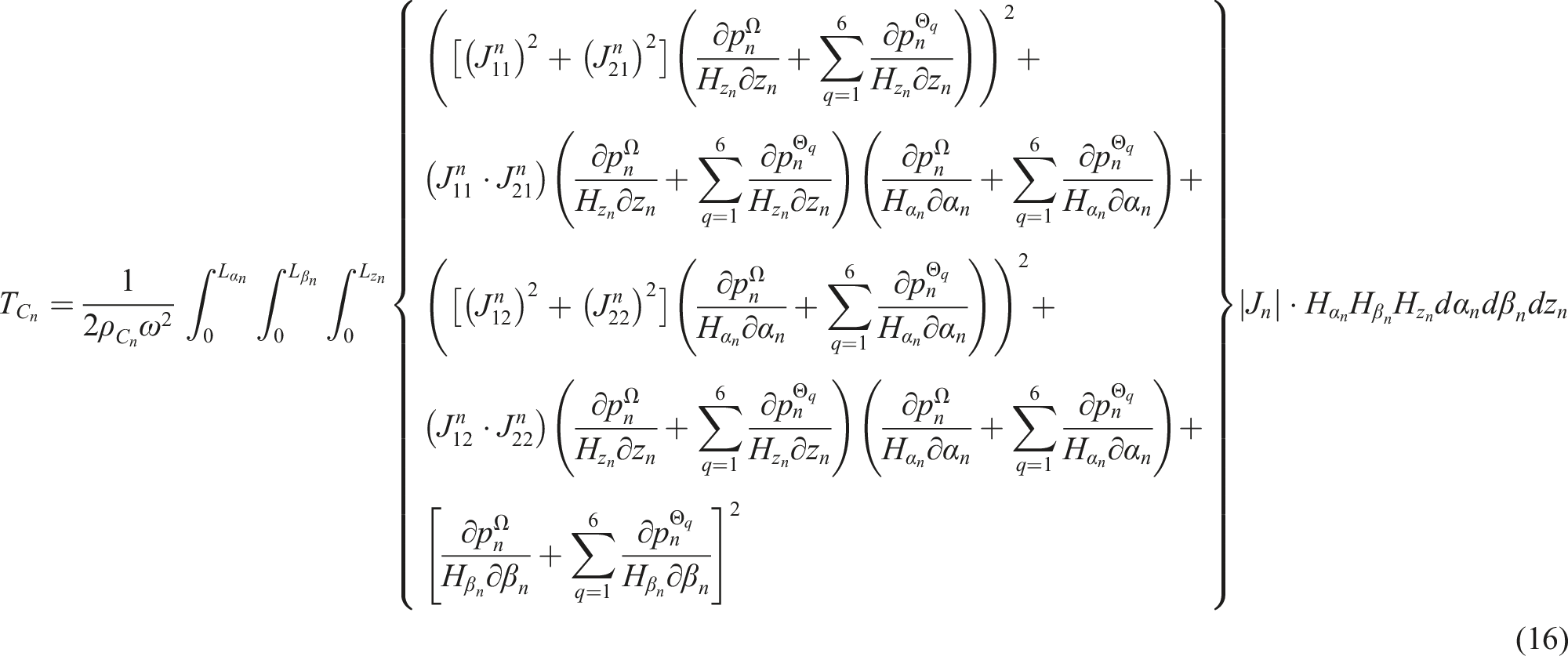
When 0 < ϑ < 2π, 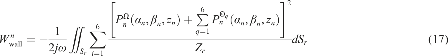$W_{\mathrm{wall}}^n$ is the energy consumed by the impedance walls, and it can be expressed as

$$W_{\mathrm{wall}}^n=-\frac{1}{2j\omega }{\displaystyle {\iint }_{S_r}{\displaystyle \sum _{i=1}^6\frac{{\left[P_n^{\mathrm{\Omega }}\left({\alpha }_n,{\beta }_n,z_n\right)+{\displaystyle \sum _{q=1}^6{P}_n^{{\mathrm{\Theta }}_q}\left({\alpha }_n,{\beta }_n,z_n\right)}\right]}^2}{Z_r}}}d{S}_r$$

(17)

$$W_{\mathrm{wall}}^n=W_{\mathrm{wal}{\mathrm{l}}_1}^n+W_{\mathrm{wal}{\mathrm{l}}_2}^n+W_{\mathrm{wal}{\mathrm{l}}_3}^n+W_{\mathrm{wal}{\mathrm{l}}_4}^n+W_{\mathrm{wal}{\mathrm{l}}_5}^n+W_{\mathrm{wal}{\mathrm{l}}_6}^n$$

(18)

where j is introduced here to designate the pure imaginary number. The area of r _th uncoupled acoustic wall is represented by S _r , and the impedance value of the corresponding acoustic wall is denoted by Z _r .

When rotation angle ϑ is 2π, the sound pressure remains consistent on the coupling interface, and the particle velocity remains continuous, hence the expression of 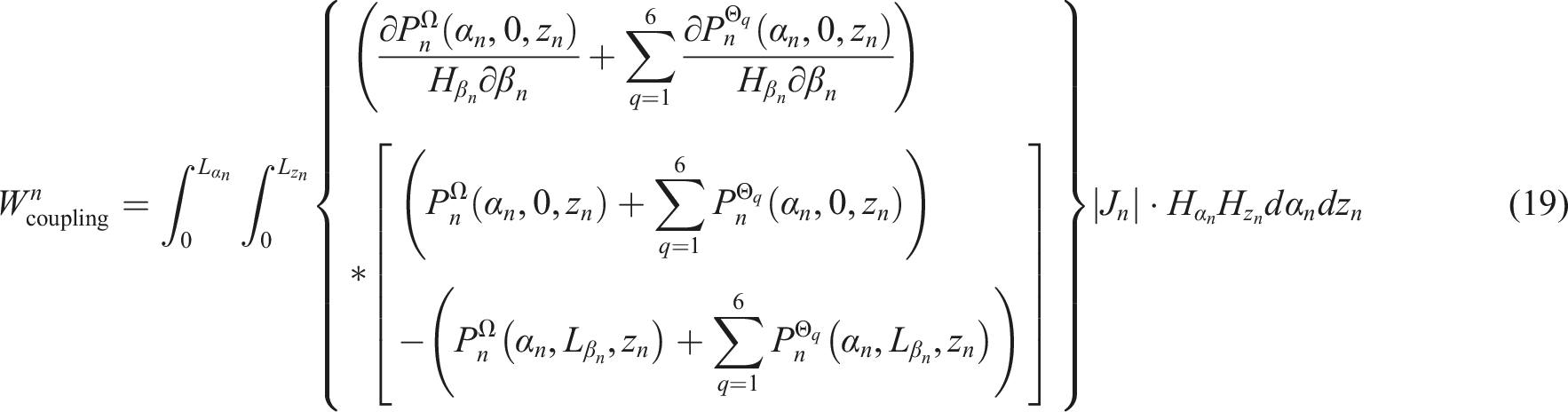$W_{\mathrm{coupling}}^n$ is written as

$$W_{\mathrm{coupling}}^n={\displaystyle {\int }_0^{L_{{\alpha }_n}}{\displaystyle {\int }_0^{L_{z_n}}\left\{\begin{array}{l}\left(\frac{\partial P_n^{\mathrm{\Omega }}\left({\alpha }_n,0,z_n\right)}{H_{{\beta }_n}\partial {\beta }_n}+{\displaystyle \sum _{q=1}^6\frac{\partial P_n^{{\mathrm{\Theta }}_q}\left({\alpha }_n,0,z_n\right)}{H_{{\beta }_n}\partial {\beta }_n}}\right)\\ \ast \left[\begin{array}{l}\left(P_n^{\mathrm{\Omega }}\left({\alpha }_n,0,z_n\right)+{\displaystyle \sum _{q=1}^6{P}_n^{{\mathrm{\Theta }}_q}\left({\alpha }_n,0,z_n\right)}\right)\\ -\left(P_n^{\mathrm{\Omega }}\left({\alpha }_n,L_{{\beta }_n},z_n\right)+{\displaystyle \sum _{q=1}^6{P}_n^{{\mathrm{\Theta }}_q}\left({\alpha }_n,L_{{\beta }_n},z_n\right)}\right)\end{array}\right]\end{array}\right\}}}\left|J_n\right|\cdot H_{{\alpha }_n}{H}_{z_n}d{\alpha }_{n}d{z}_n$$

(19)

The expression of $W_{\mathrm{sound}}^n$ can be written as

$$W_{\mathrm{sound}}^n=\frac{-1}{j\omega }{\displaystyle {\int }_0^{L_{{\alpha }_n}}{\displaystyle {\int }_0^{L_{{\beta }_n}}{\displaystyle {\int }_0^{L_{z_n}}\left\{\left(P_n^{\mathrm{\Omega }}\left({\alpha }_n,{\beta }_n,z_n\right)+{\displaystyle \sum _{q=1}^6{P}_n^{{\mathrm{\Theta }}_q}\left({\alpha }_n,{\beta }_n,z_n\right)}\right)\right\}}}}{Q}_s^n\left|J_n\right|\cdot H_{{\alpha }_n}{H}_{{\beta }_n}{H}_{z_n}d{\alpha }_{n}d{\beta }_{n}d{z}_n$$

(20)

$$Q_s^n=\frac{4\pi A}{j{\rho }_{C_n}{c}_{n}k}{\delta }_c\left(\alpha -{\alpha }_e\right){\delta }_c\left(\beta -{\beta }_e\right){\delta }_c\left(z-z_e\right)$$

(21)

in which $Q_s^n$ is the distribution function of point acoustic source acting on cavity n. A (kg/s²) is the amplitude of the point acoustic source specifically acting on point (α _e , β _e , z _e ). The acoustic wave number is represented by k, which is the ratio of the circular frequency ω to the speed of sound c _n : k = ω/c _n .

The coupling potential energy between cavity 1 and 2 marked as 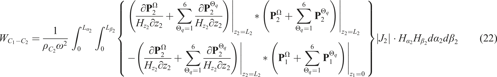$W_{C_1-C_2}$ is

$$W_{C_1-C_2}=\frac{1}{{\rho }_{C_2}{\omega }^2}{\displaystyle {\int }_0^{L_{{\alpha }_2}}{\displaystyle {\int }_0^{L_{{\beta }_2}}\left\{\begin{array}{l}{\left(\frac{\partial {\mathbf{P}}_2^{\mathrm{\Omega }}}{H_{z_2}\partial z_2}+{\displaystyle \sum _{{\mathrm{\Theta }}_q=1}^6\frac{\partial {\mathbf{P}}_2^{{\mathrm{\Theta }}_q}}{H_{z_2}\partial z_2}}\right)|}_{z_2=L_2}\ast {\left({\mathbf{P}}_2^{\mathrm{\Omega }}+{\displaystyle \sum _{{\mathrm{\Theta }}_q=1}^6{\mathbf{P}}_2^{{\mathrm{\Theta }}_q}}\right)|}_{z_2=L_2}\\ -{\left(\frac{\partial {\mathbf{P}}_2^{\mathrm{\Omega }}}{H_{z_2}\partial z_2}+{\displaystyle \sum _{{\mathrm{\Theta }}_q=1}^6\frac{\partial {\mathbf{P}}_2^{{\mathrm{\Theta }}_q}}{H_{z_2}\partial z_2}}\right)|}_{z_2=L_2}\ast {\left({\mathbf{P}}_1^{\mathrm{\Omega }}+{\displaystyle \sum _{{\mathrm{\Theta }}_q=1}^6{\mathbf{P}}_1^{{\mathrm{\Theta }}_q}}\right)|}_{z_1=0}\end{array}\right\}}}\left|J_2\right|\cdot H_{{\alpha }_2}{H}_{{\beta }_2}d{\alpha }_{2}d{\beta }_2$$

(22)

Solution procedure

Equations (15)–(22) are substituted into the Lagrange equation. According to the Ritz method, take the partial derivative of the three-dimensional unknown Fourier coefficient in the Lagrange equation, and the result is applied to be zero as follows

$$\frac{\partial U_{C_1}}{\partial {\mathbf{G}}_{mnl}}-\frac{\partial T_{C_1}}{\partial {\mathbf{G}}_{mnl}}-\frac{\partial W_{\mathbf{wall}}^1}{\partial {\mathbf{G}}_{mnl}}+\frac{\partial W_{\mathbf{coupling}}^1}{\partial {\mathbf{G}}_{mnl}}-\frac{\partial W_{C_1-C_2}}{\partial {\mathbf{G}}_{mnl}}=\frac{\partial W_{\mathbf{sound}}^1}{\partial {\mathbf{G}}_{mnl}}$$

(23)

$${\mathbf{G}}_{mnl}={\left[\begin{array}{ccccccc}{G}_{mnl}^1& G_{mnl}^2& G_{mnl}^3& G_{mnl}^4& G_{mnl}^5& G_{mnl}^6& G_{mnl}^7\end{array}\right]}^T$$

(24)

$$\frac{\partial U_{C_2}}{\partial {\mathbf{H}}_{mnl}}-\frac{\partial T_{C_2}}{\partial {\mathbf{H}}_{mnl}}-\frac{\partial W_{\mathbf{wall}}^2}{\partial {\mathbf{H}}_{mnl}}+\frac{\partial W_{\mathbf{coupling}}^2}{\partial {\mathbf{H}}_{mnl}}-\frac{\partial W_{C_1-C_2}}{\partial {\mathbf{H}}_{mnl}}=\frac{\partial W_{\mathbf{sound}}^2}{\partial {\mathbf{H}}_{mnl}}$$

(25)

$${\mathbf{H}}_{mnl}={\left[\begin{array}{ccccccc}{H}_{mnl}^1& H_{mnl}^2& H_{mnl}^3& H_{mnl}^4& H_{mnl}^5& H_{mnl}^6& H_{mnl}^7\end{array}\right]}^T$$

(26)

where ${\mathbf{G}}_{mnl}$ and ${\mathbf{H}}_{mnl}$ separately designate the unknown three-dimensional Fourier coefficient matrix of two acoustic cavities in the system.

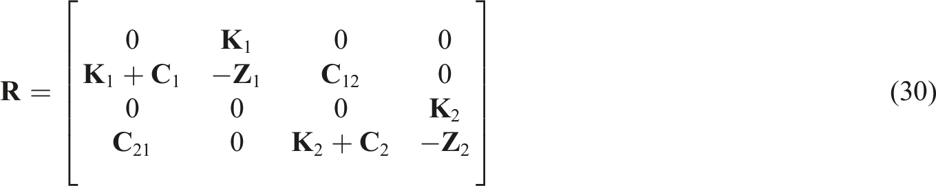
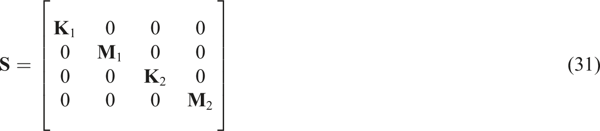
Transform equations (23)–(26) into matrix form

$$\left({\mathbf{K}}_{\mathrm{1}}\mathrm{+}{\mathbf{C}}_{\mathrm{1}}\mathrm{-}\omega {\mathbf{Z}}_{\mathrm{1}}\mathrm{-}{\omega }^{\mathrm{2}}{\mathbf{M}}_{\mathrm{1}}\right){\mathbf{G}}_{mnl}\mathrm{+}{\mathbf{C}}_{\mathrm{12}}{\mathbf{H}}_{mnl}\mathrm{=}{\mathbf{Q}}_{\mathrm{1}}$$

(27)

$$\left({\mathbf{K}}_{\mathrm{2}}\mathrm{+}{\mathbf{C}}_{\mathrm{2}}\mathrm{-}\omega {\mathbf{Z}}_{\mathrm{2}}\mathrm{-}{\omega }^{\mathrm{2}}{\mathbf{M}}_{\mathrm{2}}\right){\mathbf{H}}_{mnl}\mathrm{+}{\mathbf{C}}_{\mathrm{21}}{\mathbf{G}}_{mnl}\mathrm{=}{\mathbf{Q}}_{\mathrm{2}}$$

(28)

where K_n is the stiffness matrix of acoustic cavity n in rotary acoustic cavity coupled systems, M_n is the mass matrix of acoustic cavity n, and C_n represents the coupled matrix of acoustic cavity n. The sound field source vector of acoustic cavity n can be denoted by Q_n, and the impedance matrix of cavity n is represented by Z_n. C₁₂ and C₂₁ is the coupled matrix between acoustic cavity 1 and 2, where ${\mathbf{C}}_{12}={\mathbf{C}}_{21}^T$ .

When the point acoustic source is not arranged (Q_n = 0), equations (27) and (28) can be simultaneous to obtain the natural frequencies and modes of the rotary acoustic cavity coupled system. Calculating the equations immediately results in nonlinear solution, which is the account why they are requisite to be converted into linear equations for solution. The transformed linear equations are as follows

$$\left(\mathbf{R-}\omega \mathbf{S}\right)\mathbf{H=}0$$

(29)

$$\mathbf{R=}\left[\begin{array}{cccc}0& {\mathbf{K}}_{\mathrm{1}}& 0& 0\\ {\mathbf{K}}_{\mathrm{1}}\mathrm{+}{\mathbf{C}}_{\mathrm{1}}& \mathrm{-}{\mathbf{Z}}_{\mathrm{1}}& {\mathbf{C}}_{\mathrm{12}}& 0\\ 0& 0& 0& {\mathbf{K}}_{\mathrm{2}}\\ {\mathbf{C}}_{\mathrm{21}}& 0& {\mathbf{K}}_{\mathrm{2}}\mathrm{+}{\mathbf{C}}_{\mathrm{2}}& \mathrm{-}{\mathbf{Z}}_{\mathrm{2}}\end{array}\right]$$

(30)

$$\mathbf{S=}\left[\begin{array}{cccc}{\mathbf{K}}_{\mathrm{1}}& 0& 0& 0\\ 0& {\mathbf{M}}_{\mathrm{1}}& 0& 0\\ 0& 0& {\mathbf{K}}_{\mathrm{2}}& 0\\ 0& 0& 0& {\mathbf{M}}_{\mathrm{2}}\end{array}\right]$$

(31)

$$\mathbf{H=}\left[\begin{array}{cccc}{\mathbf{G}}_{mnl}& \omega {\mathbf{G}}_{mnl}& {\mathbf{H}}_{mnl}& \omega {\mathbf{H}}_{mnl}\end{array}\right]$$

(32)

The eigenvalue ω of the linear equations (equations (29)–(32)) is the natural frequency of the rotary acoustic cavity coupled system, and the eigenvector H is the corresponding sound pressure distribution mode.

Numerical discussions and result analysis

After constructing the unified analysis model of the rotary acoustic cavity coupled system, this section mainly verifies the convergence and accuracy of the unified analysis model, analyzes the factors that affect the natural frequency of the coupled system subject to free vibration, and studies the sound pressure response under the excitation of a point acoustic source. The example in this section chiefly employs air and water as the acoustic medium, where the density of air is defined as ρ_air = 1.21 kg/m³, the density of water is defined as ρ_water = 1000 kg/m³. The speed at which sound waves travel through air is defined as c_air = 340 m/s, and the speed at which sound waves travel through air is defined as c_water = 1480 m/s.

Unified analysis model validation

The convergence analysis and accuracy verification of the established unified analysis model for the coupled system are carried out in this part. Table 2 shows the natural frequency numerical calculation results of the cylindrical–cylindrical acoustic cavity coupled system with different truncation values obtained through the method presented in this paper. The geometric parameters of the coupled system in Table 2 are as follows: R₁ = 0.6 m, R₂ = 1.2 m, L₁ = 1m, L₂ = 2m, ϑ = 120°. The acoustic walls are all rigid. It can be seen from Table 2 that when M _c ×N _c ×L _c = 4×4×4, the natural frequency of each order basically converges.

Table 2.

Analysis of natural frequency convergence of cylindrical–cylindrical acoustic cavity coupled system.

M c ×N c ×L c	Mode number
	1	2	3	4	5	6	7	8
2×2×2	56.82	91.23	107.48	113.56	145.67	170.00	178.47	187.30
3×3×3	56.68	91.23	107.40	113.34	145.50	170.00	178.47	187.25
4×4×4	56.67	91.23	107.39	113.33	145.49	170.00	178.47	187.25
5×5×5	56.67	91.23	107.39	113.33	145.49	170.00	178.47	187.25
6×6×6	56.67	91.23	107.39	113.33	145.49	170.00	178.47	187.25
7×7×7	56.67	91.23	107.39	113.33	145.49	170.00	178.47	187.25
8×8×8	56.67	91.23	107.39	113.33	145.49	170.00	178.47	187.25
9×9×9	56.67	91.23	107.39	113.33	145.49	170.00	178.47	187.25
10×10×10	56.67	91.23	107.39	113.33	145.49	170.00	178.47	187.25
11×11×11	56.67	91.23	107.39	113.33	145.49	170.00	178.47	187.25
12×12×12	56.67	91.23	107.39	113.33	145.49	170.00	178.47	187.25
FEM	56.67	91.23	107.39	113.33	145.49	170.00	178.47	187.25

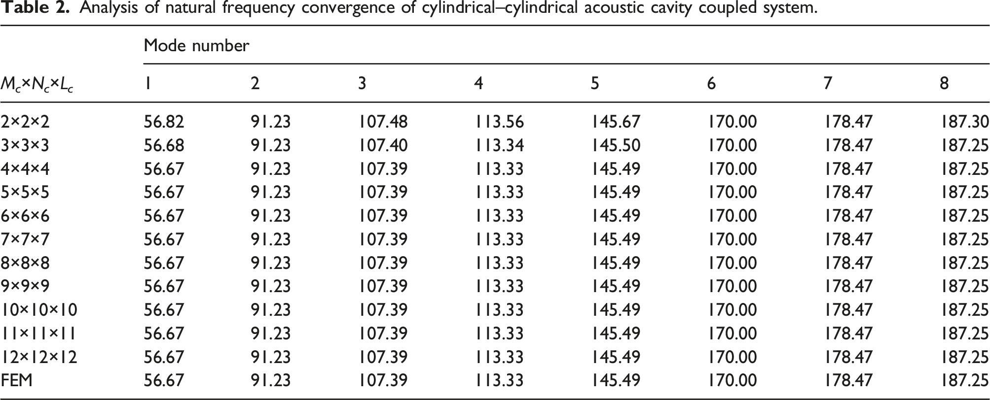
There are few references to the coupled system; the accuracy of the analytical model is verified by the finite element simulation results as a reference. The coupled system is simulated by finite element method using ABAQUS. Taking cylindrical–cylindrical acoustic cavity coupled system in Table 2 as an instance, geometric model establishment, mesh division and step type selection are shown in Figure 5. The element type of the model is AC3D20, the approximate global size of the seeds is 0.05 m, and the step type is selected as Frequency. By analyzing the simulation results listed in Table 2, the calculation results of this method are in agreement with those of finite element simulation. Therefore, it can be proved that the model of the cylindrical–cylindrical acoustic cavity coupled system constructed by the method in this paper has good convergence and accuracy.

Figure 5.

Finite element model establishment of cylindrical–cylindrical acoustic cavity coupled system. (a) model establishment and mesh division (b) step type selection.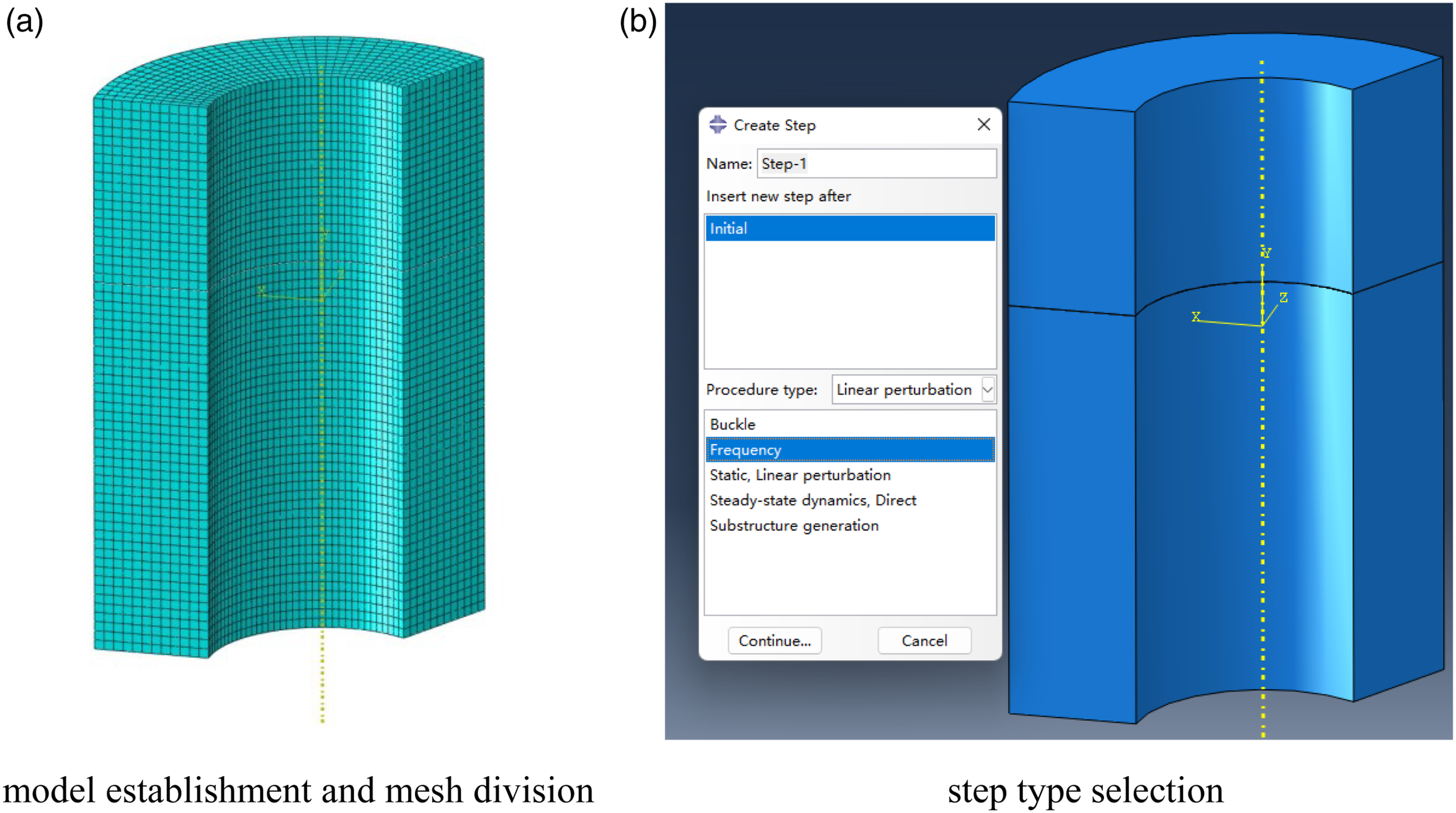

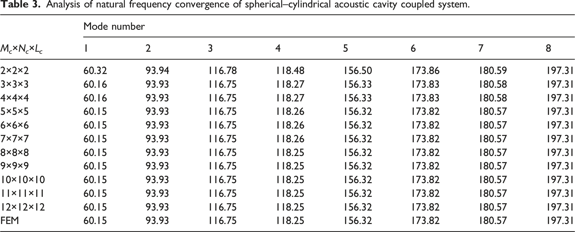
This method is also applied in finite element simulation of other rotary acoustic cavity coupled systems. The numerical results of natural frequencies of spherical–cylindrical acoustic cavity coupled system and the conical–cylindrical acoustic cavity coupled system with different truncation values are shown in Table 3 and Table 4. The geometric parameters in Table 3 are: R₁ = 0.6 m, R₂ = 1.2 m, ϕ₁ = 30°, ϕ₂ = 90°, L = 2m, ϑ = 120°, and the geometric parameters in Table 4 are: R₁ = 0.6 m, R₂ = 1.2 m, R₃ = 1.8 m, α = 30°, L₂ = 2.5 m, ϑ = 120°. The acoustic walls are all rigid. It can be known from Table 3 and Table 4 that the spherical–cylindrical acoustic cavity coupled system basically converges when M _c ×N _c ×L _c = 6×6×6, and the conical–cylindrical acoustic cavity coupled system basically converges when M _c ×N _c ×L _c = 8×8×8. Therefore, the truncation value is intended to be M _c ×N _c ×L _c = 8×8×8 in the following example calculation, and the maximum error of natural frequency of each order is less than 0.02%.

Table 3.

Analysis of natural frequency convergence of spherical–cylindrical acoustic cavity coupled system.

M c ×N c ×L c	Mode number
	1	2	3	4	5	6	7	8
2×2×2	60.32	93.94	116.78	118.48	156.50	173.86	180.59	197.31
3×3×3	60.16	93.93	116.75	118.27	156.33	173.83	180.58	197.31
4×4×4	60.16	93.93	116.75	118.27	156.33	173.83	180.58	197.31
5×5×5	60.15	93.93	116.75	118.26	156.32	173.82	180.57	197.31
6×6×6	60.15	93.93	116.75	118.26	156.32	173.82	180.57	197.31
7×7×7	60.15	93.93	116.75	118.26	156.32	173.82	180.57	197.31
8×8×8	60.15	93.93	116.75	118.25	156.32	173.82	180.57	197.31
9×9×9	60.15	93.93	116.75	118.25	156.32	173.82	180.57	197.31
10×10×10	60.15	93.93	116.75	118.25	156.32	173.82	180.57	197.31
11×11×11	60.15	93.93	116.75	118.25	156.32	173.82	180.57	197.31
12×12×12	60.15	93.93	116.75	118.25	156.32	173.82	180.57	197.31
FEM	60.15	93.93	116.75	118.25	156.32	173.82	180.57	197.31

Table 4.

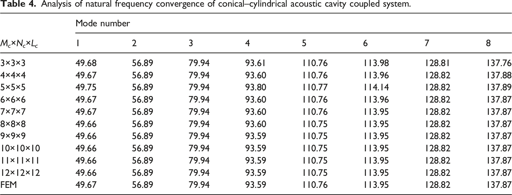
Analysis of natural frequency convergence of conical–cylindrical acoustic cavity coupled system.

M c ×N c ×L c	Mode number
	1	2	3	4	5	6	7	8
3×3×3	49.68	56.89	79.94	93.61	110.76	113.98	128.81	137.76
4×4×4	49.67	56.89	79.94	93.60	110.76	113.96	128.82	137.88
5×5×5	49.75	56.89	79.94	93.80	110.77	114.14	128.82	137.89
6×6×6	49.67	56.89	79.94	93.60	110.76	113.96	128.82	137.87
7×7×7	49.67	56.89	79.94	93.60	110.76	113.95	128.82	137.87
8×8×8	49.66	56.89	79.94	93.60	110.75	113.95	128.82	137.87
9×9×9	49.66	56.89	79.94	93.59	110.75	113.95	128.82	137.87
10×10×10	49.66	56.89	79.94	93.59	110.75	113.95	128.82	137.87
11×11×11	49.66	56.89	79.94	93.59	110.75	113.95	128.82	137.87
12×12×12	49.66	56.89	79.94	93.59	110.75	113.95	128.82	137.87
FEM	49.67	56.89	79.94	93.59	110.76	113.95	128.82	137.87

It is also essential to consider the case when the rotation angle ϑ = 360°. The first several order natural frequencies of rotary acoustic cavity coupled systems at a rotation angle of 2π obtained by present method can be found in Table 5. Except that the rotation angle ϑ is changed to 360°, the other relevant parameters of the coupling system remain unchanged. The numerical calculation results of the proposed method, shown in Table 5, are consistent with the results of the finite element simulation. This phenomenon validates the accuracy of the method when the rotation angle of the coupled system is 360°.

Table 5.

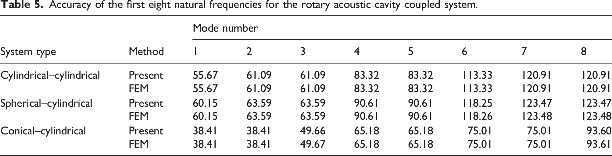
Accuracy of the first eight natural frequencies for the rotary acoustic cavity coupled system.

System type	Method	Mode number
		1	2	3	4	5	6	7	8
Cylindrical–cylindrical	Present	55.67	61.09	61.09	83.32	83.32	113.33	120.91	120.91
	FEM	55.67	61.09	61.09	83.32	83.32	113.33	120.91	120.91
Spherical–cylindrical	Present	60.15	63.59	63.59	90.61	90.61	118.25	123.47	123.47
	FEM	60.15	63.59	63.59	90.61	90.61	118.26	123.48	123.48
Conical–cylindrical	Present	38.41	38.41	49.66	65.18	65.18	75.01	75.01	93.60
	FEM	38.41	38.41	49.67	65.18	65.18	75.01	75.01	93.61

Aiming to express the sound pressure distribution of the coupled system intuitively, Figure 6 and Figure 7 separately demonstrate the first several order sound pressure mode nephograms of the coupled system obtained by the proposed method and the finite element simulation when 0 < ϑ < 360° and ϑ = 360°. The geometric parameters are consistent with Tables 2–5. It is found that the modes obtained by the two methods are consistent, which further proves the accuracy of the present method.

Figure 6.

Nephogram for sound pressure distribution of the rotary acoustic cavity coupled system when 0 < ϑ < 360°.

Figure 7.

Nephogram for sound pressure distribution of the rotary acoustic cavity coupled system when ϑ = 360°.

Natural frequency analysis

In this section, natural frequency analysis of the rotary acoustic cavity coupled system is carried out, and the effects of geometric parameters on the acoustic field characteristics of the coupled system are studied. The variations of natural frequencies of cylindrical–cylindrical acoustic cavity coupled system with different rotation angles are shown in Figure 8. The invariable geometric parameters selected for numerical calculation are: R₁ = 0.4 m, R₂ = 1m, L₁ = 1m, L₂ = 2m. As can be seen from Figure 8, the natural frequency of the same order decreases with the increase of the rotation angle ϑ under the condition of the same internal and external radius and the height of the sound cavity, but the situation changes when the rotation angle ϑ = 360°. Table 6 gives the first eight natural frequencies of the system with various rotation angles. The natural frequencies of the coupled system at ϑ = 90° include the natural frequencies of the coupled system at ϑ = 180°, and the natural frequencies of the coupled system at ϑ = 360° are numerically the same as those at ϑ = 180°. However, a closed loop is formed in the case of the coupling of the two acoustic walls, and the repeated modes are generated, resulting in the continuous extension of the natural frequencies of each order. These circumstances explain the reason why the natural frequencies rise again when ϑ = 360° in Figure 8.

Figure 8.

The variation curve of the natural frequency of cylindrical–cylindrical acoustic cavity coupled system with different rotation angles.

Table 6.

The first eight natural frequencies of the cylindrical–cylindrical acoustic cavity coupled system with various rotation angles.

ϑ	Mode number
	1	2	3	4	5	6	7	8
45°	56.67	113.33	170.00	226.67	283.33	285.83	291.39	291.73
90°	56.67	113.33	153.81	163.92	170.00	191.05	193.20	226.67
135°	56.67	104.65	113.33	119.01	154.26	170.00	199.63	200.13
180°	56.67	79.10	97.30	113.33	138.21	153.81	163.92	170.00
225°	56.67	63.51	85.12	113.33	124.65	129.92	136.93	168.47
270°	53.04	56.67	77.61	104.65	113.33	119.01	125.13	153.81
315°	45.52	56.67	72.68	90.12	106.46	113.33	122.13	133.09
360°	56.67	79.10	79.10	97.30	97.30	113.33	138.21	138.21

The first eight natural frequencies of the spherical–cylindrical acoustic cavity coupled system (a) and conical–cylindrical acoustic cavity coupled system (b) with various rotation angles are demonstrated in Table 7 and Table 8. The invariable geometric parameters selected for numerical calculation are: (a) R₁ = 0.4 m, R₂ = 1m, ϕ₁ = 30°, ϕ₂ = 90°, L = 2m; (b) R₁ = 0.5 m, R₂ = 1m, R₃ = 1.5 m, α = 30°, L₂ = 2m. The numerical calculation results in Tables 7 and 8 show that the influence of rotation angle on the acoustic field characteristics of the cylindrical acoustic cavity-cylindrical acoustic cavity coupled system is applicable to other rotary acoustic cavity coupled systems. In engineering practice, the discovery of this phenomenon is helpful to control the natural frequency of the coupled system by changing the rotation angle and number of acoustic walls, which can achieve the effect of suppressing the resonance.

Table 7.

The first eight natural frequencies of the spherical–cylindrical acoustic cavity coupled system with various rotation angles.

ϑ	Mode number
	1	2	3	4	5	6	7	8
45°	64.06	126.63	186.70	231.17	244.56	287.33	292.82	299.46
90°	64.06	126.63	155.97	174.10	186.70	208.26	221.76	244.56
135°	64.06	94.23	106.98	126.63	128.83	169.85	186.70	202.02
180°	64.06	81.31	106.43	126.63	152.87	155.97	174.10	186.70
225°	64.06	65.52	93.74	126.63	126.95	144.10	147.05	183.94
270°	54.83	64.06	85.90	106.98	126.63	128.83	139.04	155.97
315°	47.13	64.06	80.74	92.41	115.92	126.63	135.35	135.88
360°	64.06	81.31	81.31	106.43	106.43	126.63	152.87	152.87

Table 8.

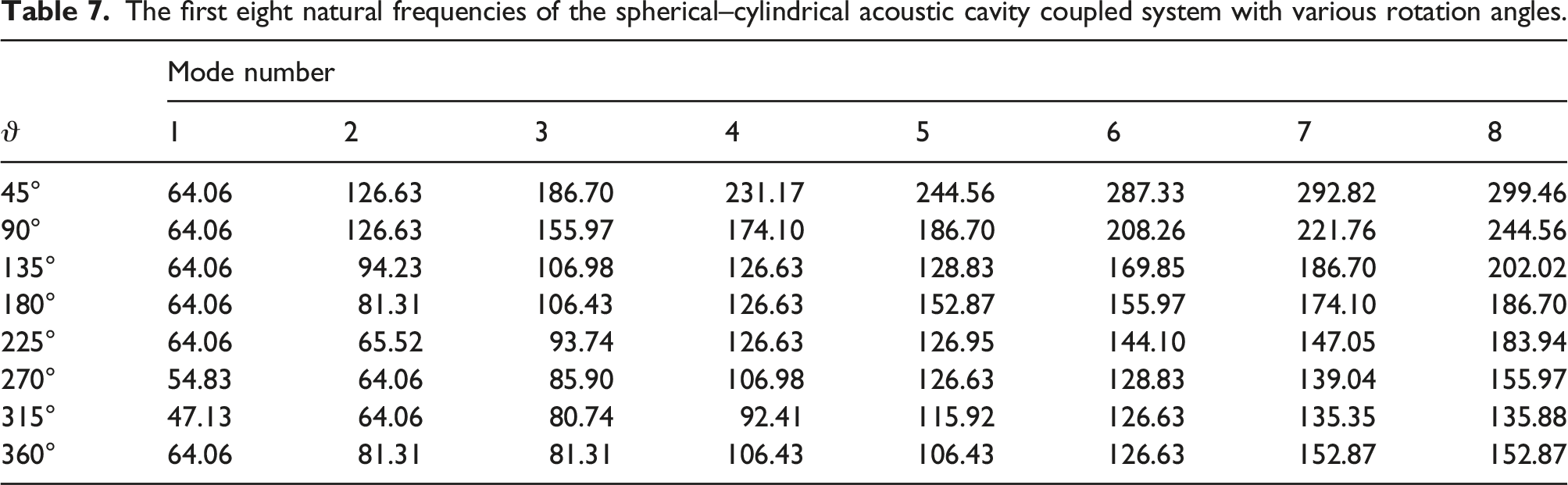
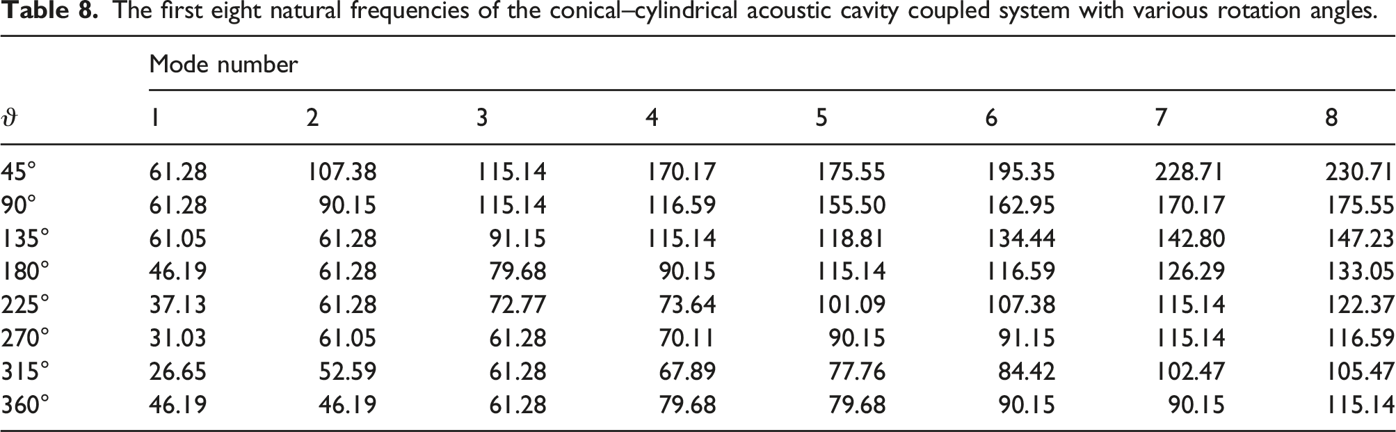
The first eight natural frequencies of the conical–cylindrical acoustic cavity coupled system with various rotation angles.

ϑ	Mode number
	1	2	3	4	5	6	7	8
45°	61.28	107.38	115.14	170.17	175.55	195.35	228.71	230.71
90°	61.28	90.15	115.14	116.59	155.50	162.95	170.17	175.55
135°	61.05	61.28	91.15	115.14	118.81	134.44	142.80	147.23
180°	46.19	61.28	79.68	90.15	115.14	116.59	126.29	133.05
225°	37.13	61.28	72.77	73.64	101.09	107.38	115.14	122.37
270°	31.03	61.05	61.28	70.11	90.15	91.15	115.14	116.59
315°	26.65	52.59	61.28	67.89	77.76	84.42	102.47	105.47
360°	46.19	46.19	61.28	79.68	79.68	90.15	90.15	115.14

Parameterization of the height L of cylindrical cavity, the apex angle ϕ of spherical cavity, and cone–apex angle α of conical cavity are also needed to analyze the influence of the parameters on the natural frequency. Figure 9 gives the tendency of the first four natural frequencies of the cavity coupled systems with different geometric parameters mentioned earlier. The known invariable geometric parameters are: (a) R₁ = 0.6 m, R₂ = 1.4 m, ϑ = 120°; (b) R₁ = 0.6 m, R₂ = 1.4 m, ϑ = 120°, ϕ₂ = 90°; (c) R₁ = 0.6 m, R₂ = 1.4 m, R₃ = 1.8 m, H = 0.4 m, ϑ = 120°. It can be seen from Figure 9 that the natural frequency of the same order of the coupled systems decreases with the increase of the heights L of the cylindrical cavity when other geometric parameters are determined. The increase of the apex angle ϕ of spherical cavity also tends to degrade the natural frequency, but the variations in the range from 0° to 90° are less significant. It is also obvious that the natural frequency of the coupled systems degrades with the decrease of cone–apex angle α.

Figure 9.

The surface diagram of the natural frequency of rotary acoustic cavity coupled system with different geometric parameters.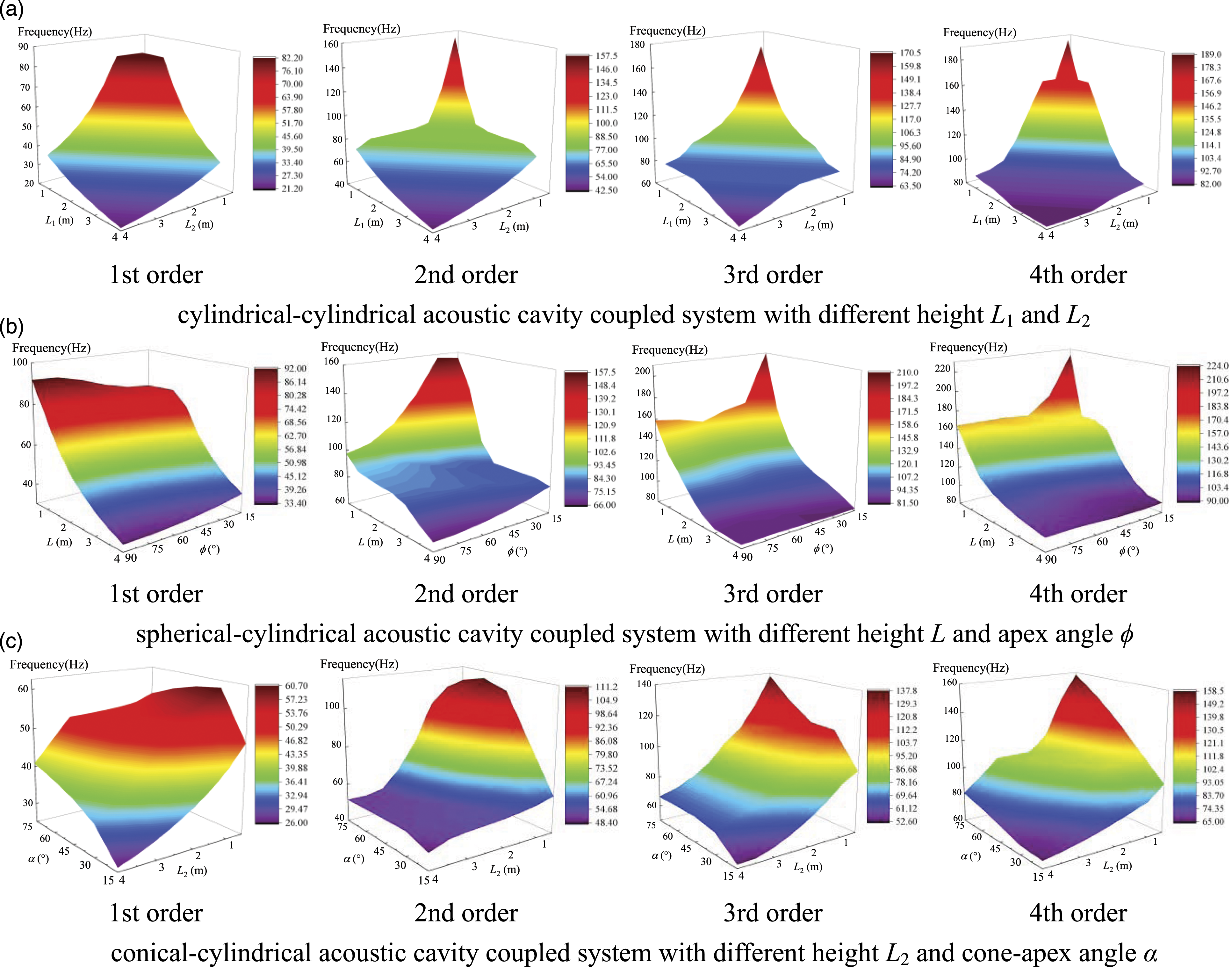

These theoretical conclusions can be applied to the structural design of workpieces. By adjusting the related geometric parameters of the acoustic cavity 1 and 2 in rotary acoustic cavity coupled systems, the natural frequency of the system can be controlled. On this basis, the dimension design of the workpiece generating the coupled system can be referenced.

Steady-state response analysis

The sound pressure response of rotary acoustic cavity coupled systems subject to the excitation of a point acoustic source is studied in this part. To simulate the sound pressure response of coupled system by finite element method in ABAQUS, another step needs to be added. The new step type is selected as steady-state dynamics, Direct. Figure 10 demonstrates the sound pressure response of cylindrical–cylindrical acoustic cavity coupled system under the excitation of a point acoustic source by present method and finite element method. The geometric parameters of this example are consistent with Table 2. The acoustic walls are all rigid. The point acoustic source is applied to (0.36 m, 1.02 m, 0.61 m) in cavity 1, the observation point 1 is located at (0.79 m, 0.43 m, 0.33 m) in cavity 1, and the observation point 2 is located at (0.26 m, 0.74 m, 0.67 m) in cavity 2. It can be found from Figure 10 that the sound pressure responses in different acoustic cavities obtained by this method subject to the excitation of point acoustic sources are basically consistent with the results of the finite element method, which verifies the accuracy of the analysis model.

Figure 10.

The sound pressure response of cylindrical–cylindrical acoustic cavity coupled system under the excitation of a point acoustic source.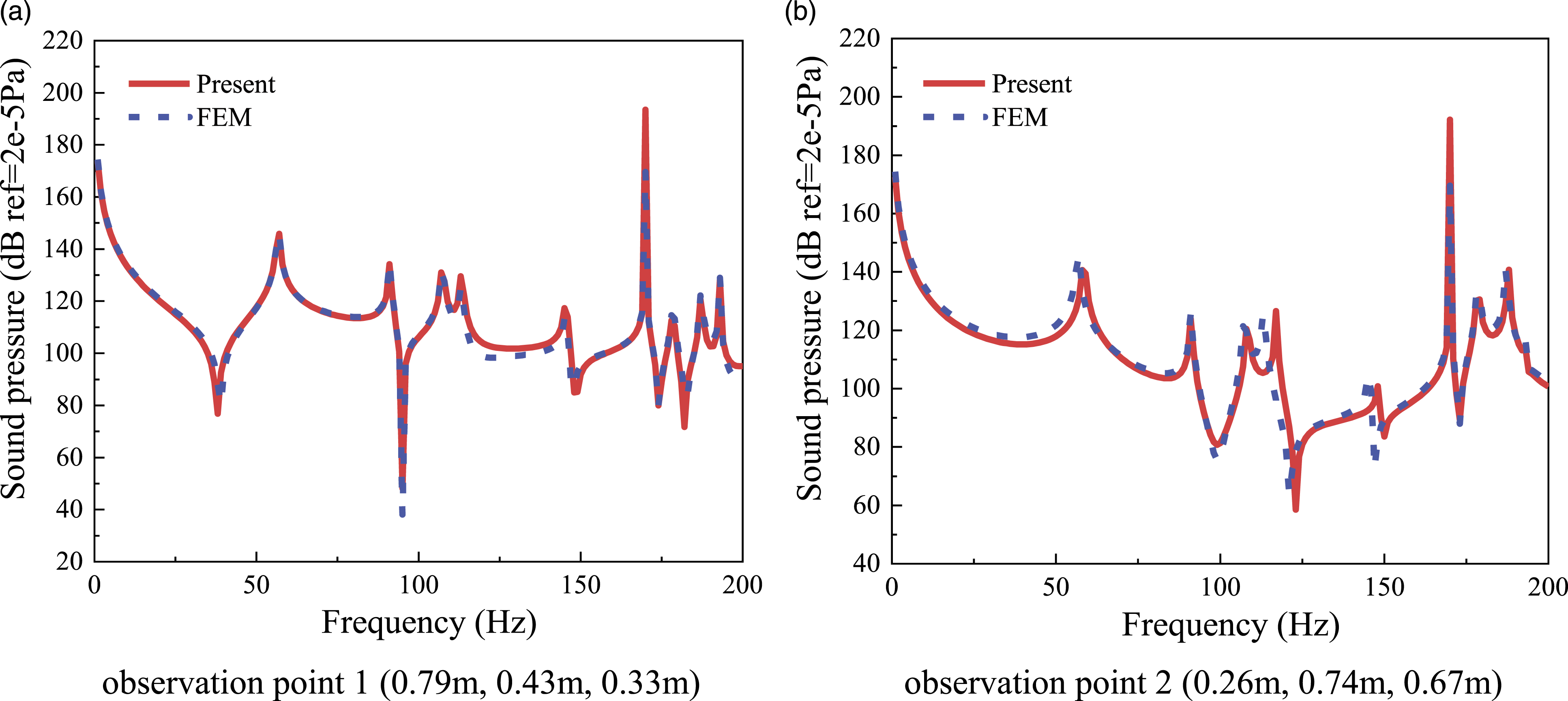

Taking cylindrical–cylindrical acoustic cavity coupled system as an instance, the influence of different acoustic media in acoustic cavities on the sound pressure response of rotary acoustic cavity coupled systems is investigated. Figure 11 presents the sound pressure response of the cylindrical–cylindrical acoustic cavity coupled system composed of different acoustic media under the excitation of a point acoustic source. The geometric parameters, acoustic walls distribution, point acoustic source location and observation point location of this example are consistent with Figure 10. As can be seen from Figure 11, in the coupled system with the same acoustic media of two cavities, if the acoustic media of one cavity changes, the peak density and magnitude of the sound pressure response curve of the whole coupled system will be changed. By comparing (a) and (b) as well as (c) and (d) in Figure 11, it can be found that, compared with the acoustic media combination of air–air, the peak density and magnitude of the sound pressure response curve of the coupled system with the acoustic media combination of air–water are significantly reduced. Compared with water–water acoustic media combination, the peak density and amplitude of sound pressure response curve of the coupled system with water–air acoustic media combination are increased. These phenomena indicate that the resonance of the sound pressure response in water is weaker than in air. Meanwhile, compared (a) and (c) as well as (b) and (d) in Figure 11, the sound pressure response curve of the air cavity within 200 Hz is consistent with that of the water cavity within 1000 Hz, indicating that different acoustic media still demonstrate some common laws. In a submarine, for example, the rotary acoustic cavity coupled system composed of air and water can form in a drainage chamber. The conclusions can be applied to the analysis of sound pressure response in the drainage chamber, which can help suppress resonance suppress resonance of the coupled system.

Figure 11.

The sound pressure response of cylindrical–cylindrical acoustic cavity coupled system under the excitation of a point acoustic source with different acoustic media.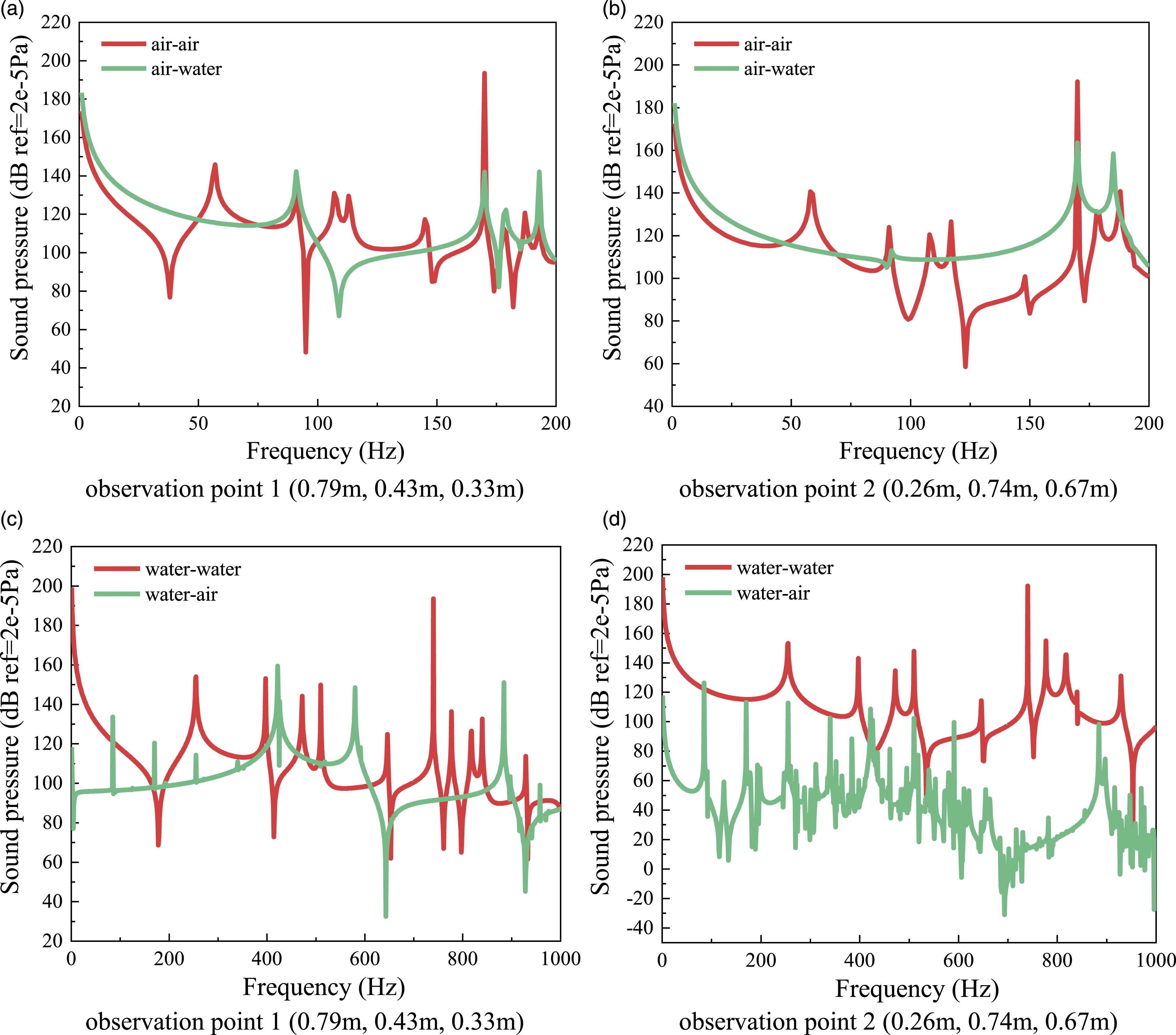

The accuracy of spherical–cylindrical acoustic cavity coupled system sound pressure response analysis model is verified in Figure 12. The geometric parameters of this example are consistent with Table 3. The acoustic walls of the spherical acoustic cavity–cylindrical acoustic cavity coupled system are all set as rigid walls. The point acoustic source is applied to (0.38 m, 0.44 m, 0.42 m) in cavity 1, the observation point 1 is located at (0.34 m, 0.95 m, 0.16 m) in cavity 1, and the observation point 2 is located at (0.22 m, 0.62 m, 1.11 m) in cavity 2. As is presented in Figure 12, the sound pressure response of the coupled system under the excitation of a point acoustic source obtained by present method are basically consistent with the results of the finite element method, which indicates this analysis model of the coupled system is precise.

Figure 12.

The sound pressure response of spherical–cylindrical acoustic cavity coupled system under the excitation of a point acoustic source.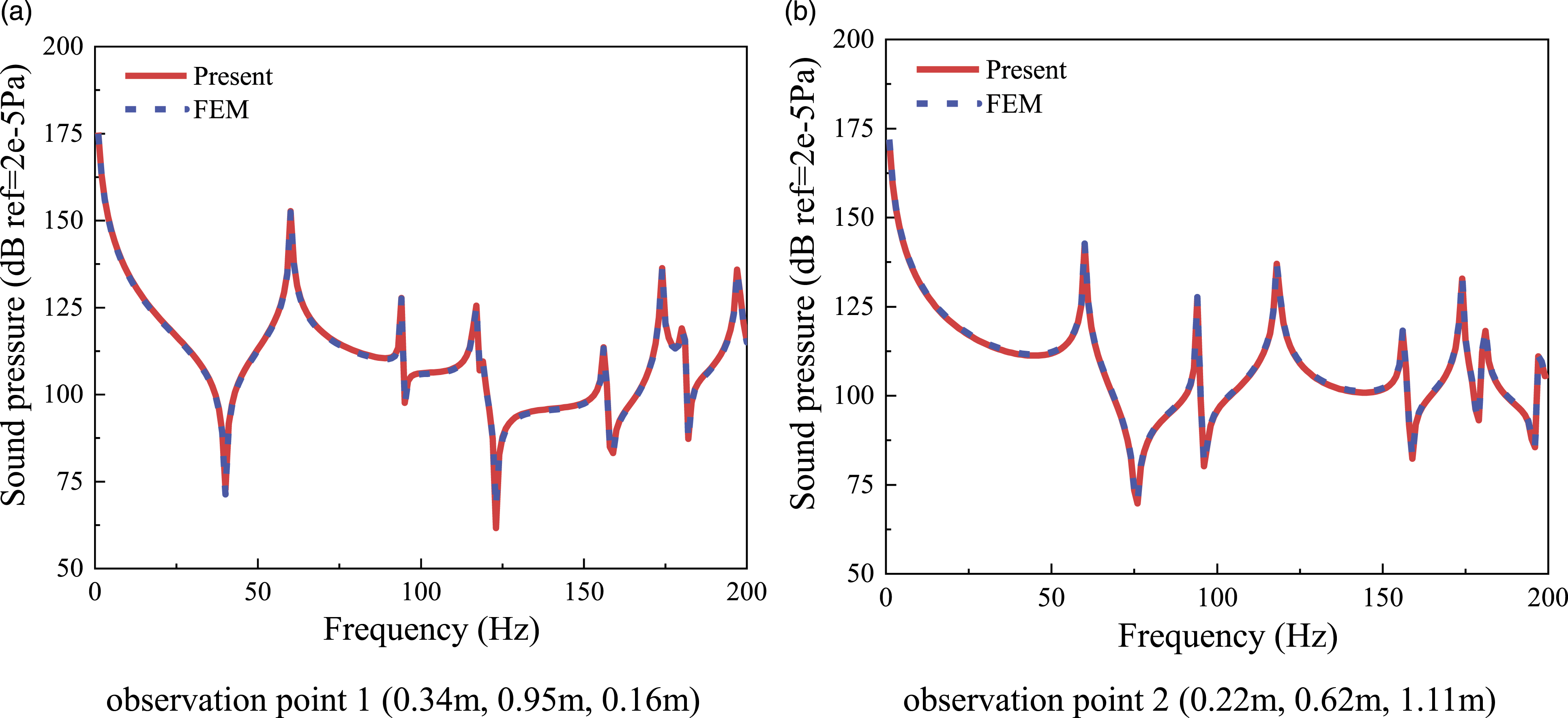

In addition to the acoustic medium of the coupled system cavity, damping and complex acoustic impedance are also introduced here to weaken the resonance phenomenon. Damping is introduced by setting the complex velocity $\tilde{c}=c_0\left(1-j{\eta }_c\right)$ , where the complex wave number is $k=k\left(1-j\xi \right)$ . According to $k^{\prime }=\omega /\tilde{c}$ , the conversion relation between damping and acoustic modal damping can be obtained: ${\eta }_c=-\xi /\left(1-j\xi \right)$ . Taking spherical–cylindrical acoustic cavity coupled system as an example, the geometric parameters, point acoustic source location and observation point location of this example are consistent with Figure 12, in which the observation point location is selected as point 1. Figure 13 (a) shows the effect of impedance wall number on the sound pressure response, where the six acoustic walls are all rigid walls. The damping values are set as $\xi =0$ , $\xi =0.001$ , and $\xi =0.01$ . We can become conscious of that the resonance phenomenon of sound pressure response is significantly suppressed when the impedance value, impedance wall number, and damping value are increased. In Figure 13 (b), the sound pressure response curves of spherical–cylindrical acoustic cavity coupled system with different impedance values are presented. The damping values are set as $\xi =0.001$ . Six acoustic walls of the coupled system are all impedance walls, and the impedance values are set as rigid, Z₁ = ρc (100 − j) and Z₂ = ρc (20 − j). Figure 13 (c) demonstrates the effect of impedance wall number on the sound pressure response. The damping values are set as $\xi =0.001$ . Whether the impedance walls are set as all rigid walls, on the top acoustic (φ₁ = 0) wall and bottom acoustic wall (s₂ = 0) of the coupled system or on all six acoustic walls, the impedance value is Z = ρc (100 − j). Meanwhile, changing the damping and complex acoustic impedance does not have distinct effect on the waveform of the sound pressure response. The conclusions can be used to design the sound source frequency and obtain the acoustic impedance and geometric parameters of sound contrast. At the same time, the acoustic impedance can be optimized by using these parameters to suppress the resonance of the coupled system.

Figure 13.

The sound pressure response of spherical–cylindrical acoustic cavity coupled system under the excitation of a point acoustic source with different conditions.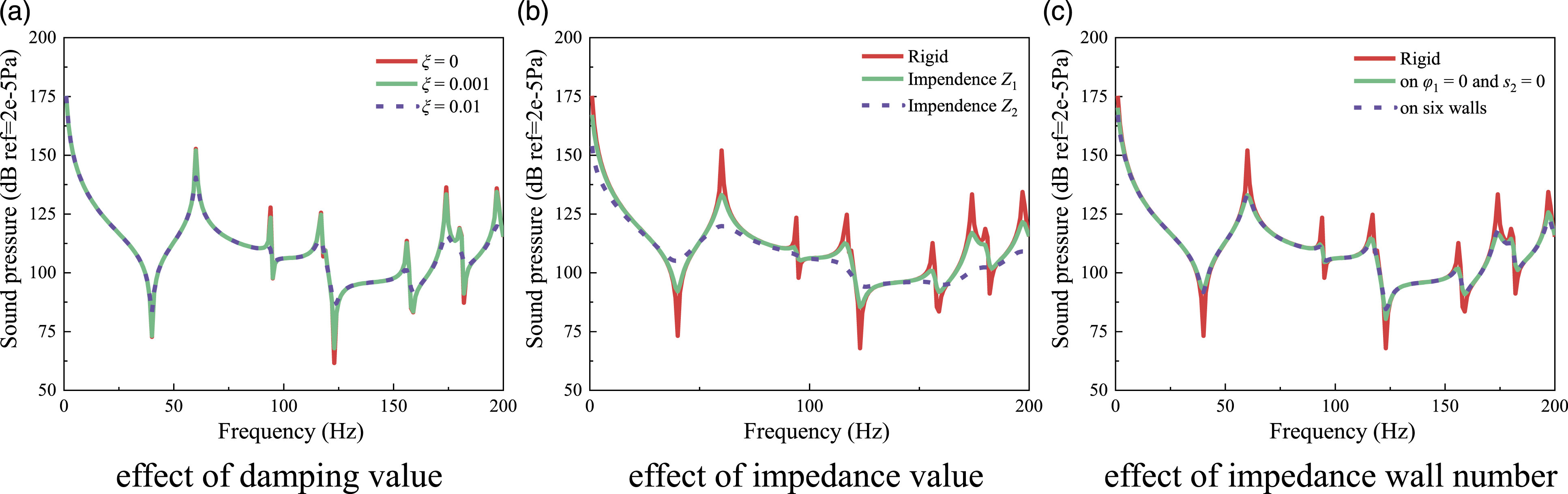

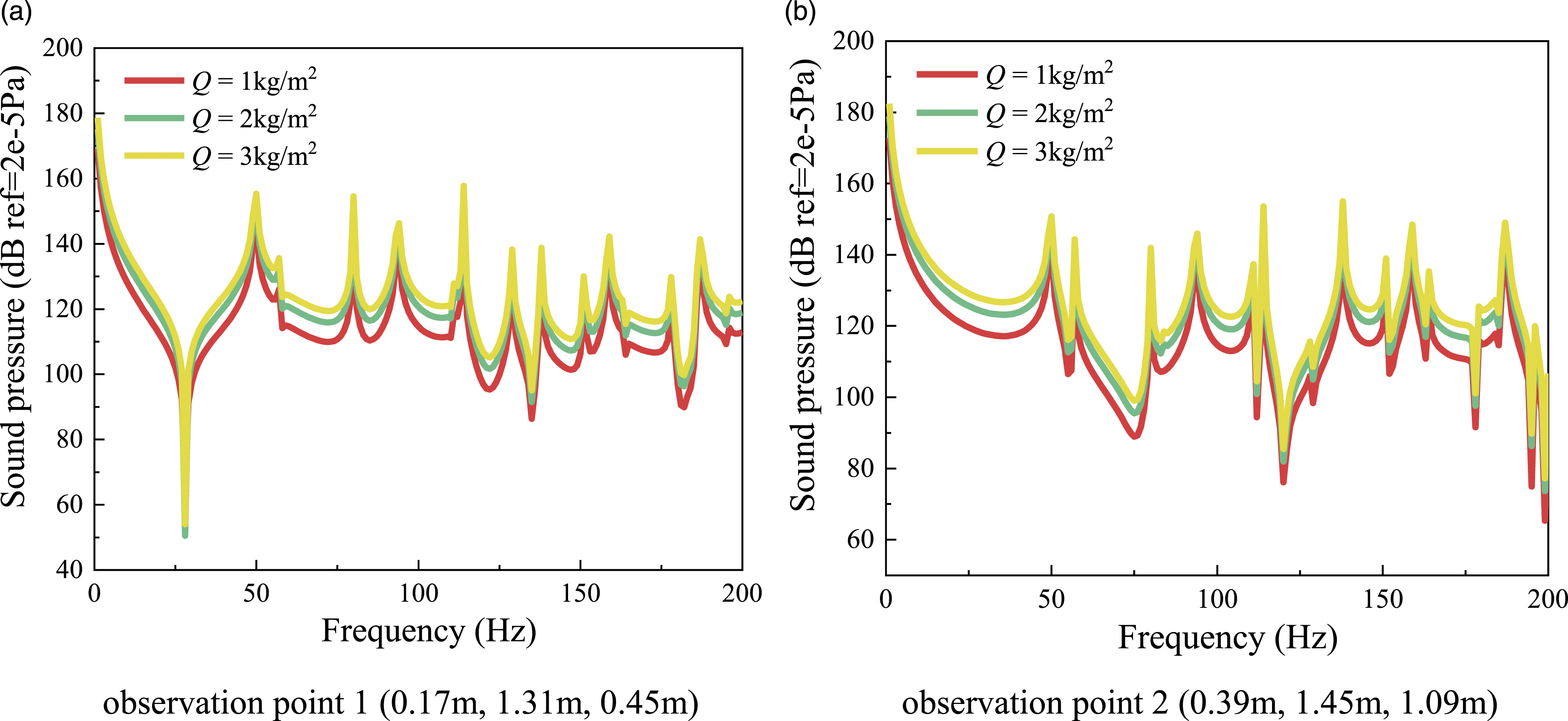
Finally, the influence of excitation amplitude on the sound pressure response is studied. Taking conical–cylindrical acoustic cavity coupled system as an instance, Figure 14 presents the sound pressure response curve of the conical–cylindrical acoustic cavity coupled system obtained by the present method and finite element method, which proves the accuracy of the coupled system sound pressure response analysis model. The geometric parameters of this example are consistent with Table 4. The acoustic walls are all rigid. The point acoustic source is applied to (0.80 m, 0.92 m, 0.74 m) in cavity 1, the observation point one is located at (0.17 m, 1.31 m, 0.45 m) in cavity 1, and the observation point two is located at (0.39 m, 1.45 m, 1.09 m) in cavity 2. After the accuracy verification, Figure 15 shows the sound pressure response curve of the coupled system with different excitation amplitudes using the same analysis model as Figure 14. The change of the amplitude of the point source contributes to the longitudinal deviation of the sound pressure response amplitude, and the sound pressure response amplitude increases with the increase of the external excitation amplitude.

Figure 14.

The sound pressure response of conical–cylindrical acoustic cavity coupled system under the excitation of a point acoustic source.

Figure 15.

The sound pressure response of conical–cylindrical acoustic cavity coupled system under the excitation of a point acoustic source with different excitation amplitudes.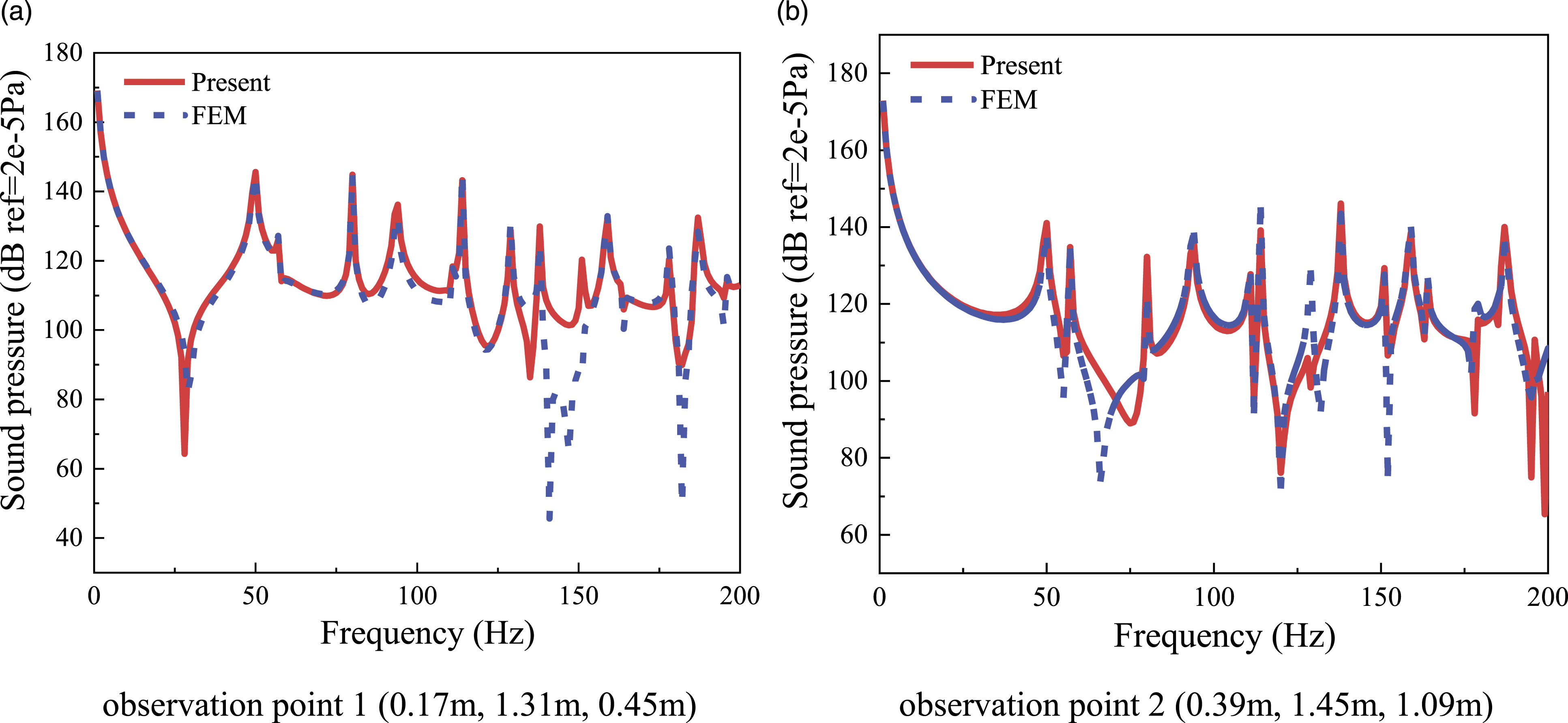

Conclusion

In this paper, a unified analysis model of the rotary acoustic cavity coupled system is established by iso-parametric transformation in finite element method. First, the admissible sound pressure functions of rotary cavities are given according to the three-dimensional improved Fourier series method. Second, the energy functional in the acoustic field of rotary cavity is constructed. Then, by introducing the coupling potential energy between the acoustic cavities, the total energy functional of the coupled system is obtained. Finally, the equation is solved by Rayleigh–Ritz method. The free vibration and steady-state response of the coupled system are studied through the numerical calculation results of the example, and the following important conclusions are obtained:

(1) The unified analysis model of rotary acoustic cavity coupled system constructed by present method has good convergence and accuracy when the truncation value Mc×Nc×Lc = 8×8×8, the maximum error of natural frequency of each order is less than 0.02%.

(2) In the condition of free vibration, the natural frequency of the rotary acoustic cavity coupled system decreases with the increase of the rotation angle. The natural frequency of the coupled system decreases with the increase of the heights of cylindrical cavities, the natural frequency decreases with the increase of the height of cylindrical cavity and the apex angle of spherical cavity, and the natural frequency decreases with the increase of cylindrical cavity height and the decrease of cone–apex angle of conical cavity.

(3) In the rotary acoustic cavity coupled system, the resonance of the sound pressure response of in water is weaker than in air. The sound pressure response amplitude decreases with the decrease of impedance value and the increase of the impedance wall number, but the variation does not affect the waveform of the response. Meanwhile, the sound pressure response amplitude increases with the increase of the external excitation amplitude.