Nonlinear vibration of an orthotropic moving membrane

Abstract

This paper addresses the dynamic behaviours of an orthotropic moving membrane. Considering the material properties of the membrane, a mathematical model is developed via the von Karman’s large deflection theory. The dynamic behaviours are demonstrated by numerical analysis based on the Runge–Kutta fourth-order method. These numerical examples provide important insights into the impacts of the velocity, aspect ratio and orthotropic coefficient on the nonlinear dynamics of the orthotropic membrane.

Introduction

In printing, the membrane is the main substrate, and the stability of the membrane transmission process is the key to determining the quality of printed products. At present, investigations of printed membranes generally assume that they are isotropic. However, in terms of material properties, the membranes are orthotropic in practical applications. Therefore, the nonlinear vibration of the orthotropic membrane is investigated to provide a theoretical basis for the parameter selection of printing equipment.

A considerable amount of literature has been published on the vibration characteristics of the orthotropic plates, panels and shells. Hatami et al. ¹ applied classic plate theory to investigate the free vibration of a symmetric laminated plate under the plane force. Zhang ² developed a novel accurate analysis method for the vibration of orthotropic plates. Jeronen ³ applied the linearized Kirchhoff plate theory to calculate the critical velocity of orthotropic thin plates under nonuniform tension. Rai and Gupta ⁴ investigated the nonlinear vibration of a polar-orthotropic circular plate under moving point loads. Ghulghazaryan ⁵ investigated the free vibration of an orthotropic cylindrical panel via the generalized Kantorovich–Vlasov method. Rogério ⁶ combined the active face with a honeycomb to analyse the vibration of orthotropic laminated panels. Latifov ⁷ investigated the vibration of heterogeneous orthotropic cylindrical shells and obtained the effect of physical parameters and various geometries on the frequency response. Civalek ⁸ studied the nonlinear vibration of shallow spherical shells and analysed the damping effect on vibration characteristics.

Unlike the plate-like materials, investigations connected with the vibration characteristics of the membrane neglects the bending stiffness due to its flexibility. Large numbers of researches assumed that paper is an isotropic material. However, considering the fibre structure of paper, it can be described as an orthotropic material ⁹ in the production process. Marynowski ¹⁰ compared experimental data with theoretical calculations and verified that the paper is an orthotropic material. A great deal of previous researches into the vibration characteristic of orthotropic membrane has focussed on the prestressed condition, impact loading and modal coupling. Kurki ¹¹ considered the origin of in-plane stresses in continuous webs. Liu et al.^{12, 13} analysed the damped vibration and nonlinear dynamics of a prestressed orthotropic membrane structure subjected to impact loading, and numerically calculated its nonlinear vibration response.^14,15 Ahmadi ¹⁶ studied nonlinear vibrations of prestressed orthotropic membranes. Zheng et al. ¹⁷ developed the mean square value function of orthotropic membranes with random impact load. Li et al. ¹⁸ applied the KBM perturbation method to derive the motion governing equations of prestressed orthotropic membranes under impact load. In addition, they used the same method to investigate the random response and reliability of orthotropic membrane structures. The effect of preload, radius and impact velocity on the reliability of structure were also examined in Refs.[19,20]. They also considered the coupling between different modes and analysed free vibrations of orthotropic membranes in.Ref. [21]. Wetherhold and Padliya ²² obtained the natural frequency of specific orthotropic membranes and provided strategies to evaluate the initial tension from the measured vibration frequency. These mentioned studies are mainly about the vibration characteristics of static membranes.

In printing process, the membrane is however transported with a moving velocity. In view of all that has been mentioned so far, previous studies mainly focus on the vibration of membranes without transmission speed. The effect of material properties and transport velocity on the dynamical behaviours of orthotropic moving membranes (mainly paper) has been rarely observed. The difference in material characteristics would make the vibration characteristics more complicated. Herein, the bifurcation and chaos of an orthotropic moving membrane are considered. The parameter effects on the nonlinear dynamics of the orthotropic membrane are also highlighted.

Establishing an equation for an orthotropic moving membrane

In this section, a mathematical model is established based on the D'Alembert principle and von Karman’s large deflection theory, and nonlinear vibration equations are obtained to characterize the nonlinear vibration of an orthotropic moving membrane.

In Figure 1, a rectangular membrane with in-plane dimensions a and b and thickness h is considered. v is the moving velocity of the membrane, $\rho$ is areal density, $\overline{w}(x,y,t)$ represents the transverse deflection function and $\overline{p}\cos \varpi t$ signifies concentrated external excitation.

Figure 1.

Mechanical modelling of an orthotropic moving membrane.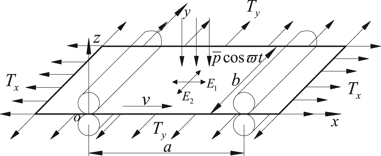

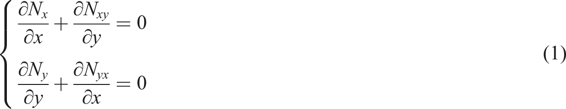
The membrane satisfies the following equilibrium differential functions ²³ :

$$\{\begin{array}{c}\frac{\partial N_x}{\partial x}+\frac{\partial N_{xy}}{\partial y}=0\\ \frac{\partial N_y}{\partial y}+\frac{\partial N_{yx}}{\partial x}=0\end{array}$$

(1)

The elastic curved surface differential equation of a membrane can be written as:

$$\rho \left(\frac{{\partial }^2\overline{w}}{\partial t^2}+2v\frac{{\partial }^2\overline{w}}{\partial x\partial t}+v^2\frac{{\partial }^2\overline{w}}{\partial x^2}\right)-N_x\frac{{\partial }^2\overline{w}}{\partial x^2}-N_y\frac{{\partial }^2\overline{w}}{\partial y^2}-2N_{xy}\frac{{\partial }^2\overline{w}}{\partial x\partial y}-\overline{p}\cos \varpi t=0$$

(2)

where N _y , N _x , N _yx and N _xy represent the internal forces of a membrane at each unit length.

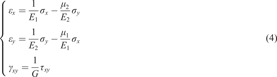
The membrane is an orthotropic material, and one can obtain ^20,21:

$$E_1{\mu }_2=E_2{\mu }_1$$

(3)

where ${\mu }_1$ and ${\mu }_2$ represent the Poisson’s ratio along the x-axis and y-axis, respectively and E₁ and E ₂ denote the elastic modulus along the x-axis and y-axis, respectively.

The stress strain equation is given as

$$\{\begin{array}{l}{\epsilon }_x=\frac{1}{E_1}{\sigma }_x-\frac{{\mu }_2}{E_2}{\sigma }_y\\ {\epsilon }_y=\frac{1}{E_2}{\sigma }_y-\frac{{\mu }_1}{E_1}{\sigma }_x\\ {\gamma }_{xy}=\frac{1}{G}{\tau }_{xy}\end{array}$$

(4)

where ${\sigma }_x$ and ${\sigma }_y$ denote the normal stresses along the x-axis and y-axis, ${\tau }_{xy}$ is the shear stress and G signifies the shear modulus.

Considering the effect of damping, the nonlinear governing equations of orthotropic membranes under external excitation are derived from the D'Alembert principle and von Karman’s large deflection theory:

$$\rho \hspace{0.17em}\left(\frac{{\partial }^2\overline{w}}{\partial t^2}+2v\frac{{\partial }^2\overline{w}}{\partial x\partial t}+v^2\frac{{\partial }^2\overline{w}}{\partial x^2}\right)-N_x\frac{{\partial }^2\overline{w}}{\partial x^2}-N_y\frac{{\partial }^2\overline{w}}{\partial y^2}-2N_{xy}\frac{{\partial }^2\overline{w}}{\partial x\partial y}+\vartheta \frac{\partial \overline{w}}{\partial t}-\overline{p}\cos \varpi t=0$$

(5a)

$$\frac{1}{E_{1}h}\frac{{\partial }^2{N}_x}{\partial y^2}-\frac{{\mu }_2}{E_{2}h}\frac{{\partial }^2{N}_y}{\partial y^2}-\frac{{\mu }_1}{E_{1}h}\frac{{\partial }^2{N}_x}{\partial x^2}+\frac{1}{E_{2}h}\frac{{\partial }^2{N}_y}{\partial x^2}-\frac{1}{Gh}\frac{{\partial }^2{N}_{xy}}{\partial x\partial y}={\left(\frac{{\partial }^2\overline{w}}{\partial x\partial y}\right)}^2-\frac{{\partial }^2\overline{w}}{\partial x^2}\frac{{\partial }^2\overline{w}}{\partial y^2}$$

(5b)

where $\vartheta$ is the damping constant.

The internal force function $\Phi (x,y)$ is

$$\{\begin{array}{c}{N}_x=\frac{{\partial }^2\Phi }{\partial y^2}\\ N_y=\frac{{\partial }^2\Phi }{\partial x^2}\\ N_{xy}=-\frac{{\partial }^2\Phi }{\partial x\partial y}\end{array}$$

(6)

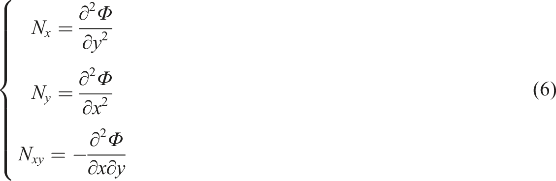
The membrane is homogeneous and soft, and shear stress can be considered negligible, thereby supposing $N_{xy}=0$ .

Substituting equation (6) into equation (5a) and (5b) yields

$$\rho \left(\frac{{\partial }^2\overline{w}}{\partial t^2}+2v\frac{{\partial }^2\overline{w}}{\partial x\partial t}+v^2\frac{{\partial }^2\overline{w}}{\partial x^2}\right)-\frac{{\partial }^2\Phi }{\partial y^2}\frac{{\partial }^2\overline{w}}{\partial x^2}-\frac{{\partial }^2\Phi }{\partial x^2}\frac{{\partial }^2\overline{w}}{\partial y^2}+\vartheta \frac{\partial \overline{w}}{\partial t}-\overline{p}\cos \varpi t=0$$

(7a)

$$\frac{1}{E_1}\frac{{\partial }^4\Phi }{\partial y^4}+\frac{1}{E_2}\frac{{\partial }^4\Phi }{\partial x^4}=h\left[{\left(\frac{{\partial }^2\overline{w}}{\partial x\partial y}\right)}^2-\frac{{\partial }^2\overline{w}}{\partial x^2}\frac{{\partial }^2\overline{w}}{\partial y^2}\right]$$

(7b)

The governing equation can also be derived by variational principle. ²⁴

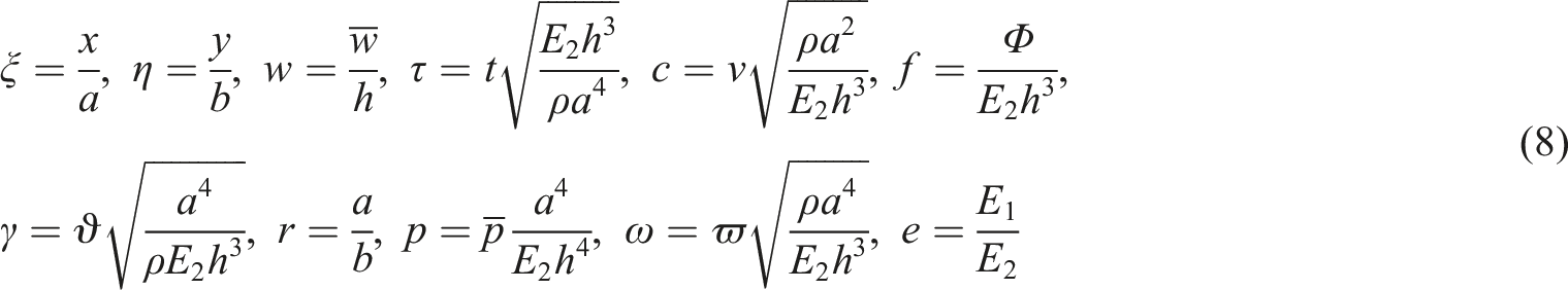
The nondimensional parameters are

$$\begin{array}{l}\xi =\frac{x}{a},\eta =\frac{y}{b},w=\frac{\overline{w}}{h},\tau =t\sqrt{\frac{E_2{h}^3}{\rho a^4}},c=v\sqrt{\frac{\rho a^2}{E_2{h}^3}},f=\frac{\Phi }{E_2{h}^3},\\ \gamma =\vartheta \sqrt{\frac{a^4}{\rho E_2{h}^3}},r=\frac{a}{b},p=\overline{p}\frac{a^4}{E_2{h}^4},\omega =\varpi \sqrt{\frac{\rho a^4}{E_2{h}^3}},e=\frac{E_1}{E_2}\end{array}$$

(8)

where c is the nondimensional velocity, γ is the nondimensional damping constant, e denotes the orthotropic coefficient and r signifies the aspect ratio.

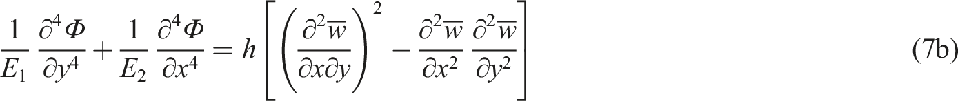
Then, equation (7a) and (7b) can be rewritten as:

$$\left(\frac{{\partial }^{2}w}{\partial {\tau }^2}+2c\frac{{\partial }^{2}w}{\partial \xi \partial \tau }+c^2\frac{{\partial }^{2}w}{\partial {\xi }^2}\right)-r^2\frac{{\partial }^{2}f}{\partial {\eta }^2}\frac{{\partial }^{2}w}{\partial {\xi }^2}-r^2\frac{{\partial }^{2}f}{\partial {\xi }^2}\frac{{\partial }^{2}w}{\partial {\eta }^2}+\gamma \frac{\partial w}{\partial \tau }=p\cos \omega \tau$$

(9a)

$$\frac{{\partial }^{4}f}{\partial {\xi }^4}+\frac{r^4}{e}\frac{{\partial }^{4}f}{\partial {\eta }^4}=r^2{\left(\frac{{\partial }^{2}w}{\partial \xi \partial \eta }\right)}^2-r^2\frac{{\partial }^{2}w}{\partial {\xi }^2}\frac{{\partial }^{2}w}{\partial {\eta }^2}$$

(9b)

The boundary conditions ²⁵ are

$$\xi =\mathrm{0,1}:\frac{{\partial }^{2}f}{\partial {\eta }^2}=1,\frac{{\partial }^{2}f}{\partial \xi \partial \eta }=0,\omega =0$$

(10a)

$$\eta =\mathrm{0,1}:\frac{{\partial }^{2}f}{\partial {\xi }^2}=1,\frac{{\partial }^{2}f}{\partial \xi \partial \eta }=0,\omega =0$$

(10b)

The Galerkin method

In this section, the Galerkin Method is employed to discretize the nonlinear vibration equations obtained from the established model, and the ordinary differential equations can be derived for the subsequent numerical analysis.

The solution satisfying the boundary conditions is given as ¹⁹

$$w\left(\xi ,\eta ,\tau \right)={\displaystyle \sum _{i=1}^{M_i}{\displaystyle \sum _{j=1}^{M_j}{q}_{ij}\left(\tau \right)}}\sin \left(i\pi \xi \right)\sin \left(j\pi \eta \right)$$

(11)

In the case of $M_i=2$ and $M_j=1$ , the function can embody the response characteristics of the system

$$w\left(\xi ,\eta ,\tau \right)=q_{11}\left(\tau \right)\sin \left(\pi \xi \right)\sin \left(\pi \eta \right)+q_{21}\left(\tau \right)\sin \left(2\pi \xi \right)\sin \left(\pi \eta \right)$$

(12)

The stress function is stated as

$$f\left(\xi ,\eta ,\tau \right)=\frac{{\xi }^2}{2}+\frac{{\eta }^2}{2}+{\displaystyle \sum _{i=1}^{M_i}{\displaystyle \sum _{j=1}^{M_j}{f}_{ij}\left(\tau \right)}}{\sin }^2\left(\mathit{i}\pi \xi \right){\sin }^2\left(\mathit{j}\pi \eta \right)$$

(13)

where $f_{ij}\left(\tau \right)$ denotes the unknown coefficient.

In the case of i=1, j = 1 and i = 2, j = 1, equation (13) is described as

$$f\left(\xi ,\eta ,\tau \right)=\frac{{\xi }^2}{2}+\frac{{\eta }^2}{2}+f_{11}\left(\tau \right){\sin }^2\left(\pi \xi \right){\sin }^2\left(\pi \eta \right)+f_{21}\left(\tau \right){\sin }^2\left(2\pi \xi \right){\sin }^2\left(\pi \eta \right)$$

(14)

where $f_{11}\left(\tau \right)$ and $f_{21}\left(\tau \right)$ denotes the unknown coefficient.

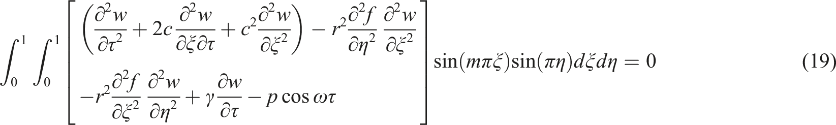
The following equation can be obtained by substituting equations (12) and (14) into equation (9a) via the Galerkin method as

$${\displaystyle {\int }_0^1{\displaystyle {\int }_0^1\left[\frac{{\partial }^{4}f}{\partial {\xi }^4}+\frac{r^4}{e}\frac{{\partial }^{4}f}{\partial {\eta }^4}-r^2{\left(\frac{{\partial }^{2}w}{\partial \xi \partial \eta }\right)}^2+r^2\frac{{\partial }^{2}w}{\partial {\xi }^2}\frac{{\partial }^{2}w}{\partial {\eta }^2}\right]}}{\sin }^2\left(i\pi \xi \right){\sin }^2\left(j\pi \eta \right)d\xi d\eta =0$$

(15)

Through two integrations of equation (15), one can obtain

$$\left(6e+6r^4\right)f_{11}\left(\tau \right)+4r^4{f}_{21}\left(\tau \right)+r^{2}e{q}_{11}^2\left(\tau \right)+2r^{2}e{q}_{21}^2\left(\tau \right)=0$$

(16a)

$$8r^4{f}_{11}\left(\tau \right)+\left(192e+12r^4\right)f_{21}\left(\tau \right)+r^{2}e{q}_{11}^2\left(\tau \right)+8r^{2}e{q}_{21}^2\left(\tau \right)=0$$

(16b)

Then, $f_{11}\left(\tau \right)$ and $f_{21}\left(\tau \right)$ can be expressed as

$$f_{11}\left(\tau \right)=\frac{-\left(96r^2{e}^2+4r^{6}e\right)q_{11}^{2}q\left(\tau \right)+\left(4r^{6}e-192r^2{e}^2\right)q_{21}^2\left(\tau \right)}{20r^8+612e{r}^4+576e^2}=\beta \left[{\alpha }_{11}{q}_{11}^2\left(\tau \right)+{\alpha }_{12}{q}_{21}^2\left(\tau \right)\right]$$

(17)

$$f_{21}\left(\tau \right)=\frac{\left(r^{6}e-3r^2{e}^2\right)q_{11}^2\left(\tau \right)-\left(16r^{6}e+24r^2{e}^2\right)q_{21}^2\left(\tau \right)}{20r^8+612e{r}^4+576e^2}=\beta \left[{\alpha }_{21}{q}_{11}^2\left(\tau \right)+{\alpha }_{22}{q}_{21}^2\left(\tau \right)\right]$$

(18)

where ${\alpha }_{11}=-\left(96r^2{e}^2+4r^{6}e\right)$ , ${\alpha }_{12}=4r^{6}e-192r^2{e}^2$ , ${\alpha }_{21}=r^{6}e-3r^2{e}^2$ , ${\alpha }_{22}=-\left(16r^{6}e+24r^2{e}^2\right)$ and $\beta =\frac{1}{20r^8+612r^{4}e+576e^2}$ .

The following equation can also be obtained by substituting equations (12) and (14) into equation (9a) via the Galerkin method as

$${\displaystyle {\int }_0^1{\displaystyle {\int }_0^1\left[\begin{array}{l}\left(\frac{{\partial }^{2}w}{\partial {\tau }^2}+2c\frac{{\partial }^{2}w}{\partial \xi \partial \tau }+c^2\frac{{\partial }^{2}w}{\partial {\xi }^2}\right)-r^2\frac{{\partial }^{2}f}{\partial {\eta }^2}\frac{{\partial }^{2}w}{\partial {\xi }^2}\\ -r^2\frac{{\partial }^{2}f}{\partial {\xi }^2}\frac{{\partial }^{2}w}{\partial {\eta }^2}+\gamma \frac{\partial w}{\partial \tau }-p\cos \omega \tau \end{array}\right]}}\sin \left(m\pi \xi \right)\sin \left(\pi \eta \right)d\xi d\eta =0$$

(19)

In the case of m = 1 and m = 2, the state equations of the moving orthotropic membrane are

$$\frac{d^2{q}_{11}}{d{t}^2}+G_{11}\frac{d{q}_{21}}{dt}+{\gamma }_1\frac{d{q}_{11}}{dt}+k_{11}{q}_{11}+k_{12}{q}_{11}^2+k_{13}{q}_{11}{q}_{21}^2=P\cos \omega \tau$$

(20a)

$$\frac{d^2{q}_{21}}{d{t}^2}+G_{21}\frac{d{q}_{11}}{dt}+{\gamma }_1\frac{d{q}_{21}}{dt}+k_{21}{q}_{21}+k_{22}{q}_{21}^2+k_{23}{q}_{11}^2{q}_{21}=0$$

(20b)

where $G_{11}=-\frac{16c}{3}$ , $k_{11}=2{\pi }^2{r}^2-{\pi }^2{c}^2$ , $k_{12}=-\frac{{\pi }^4{r}^2\beta }{2}\left(3{\alpha }_{11}+{\alpha }_{21}\right)$ , $k_{13}=-\frac{{\pi }^4{r}^2\beta }{2}\left(3{\alpha }_{12}+{\alpha }_{22}\right)$ , ${\gamma }_1=\frac{\gamma }{4}$ , $P=\frac{16\text{p}}{{\pi }^2}$ , $G_{21}=\frac{16c}{3}$ , $k_{21}=5{\pi }^2{r}^2-4{\pi }^2{c}^2$ , $k_{22}=-2{\pi }^4{r}^2\beta \left({\alpha }_{12}+3{\alpha }_{22}\right)$ and $k_{23}=-2{\pi }^4{r}^2\beta \left({\alpha }_{11}+3{\alpha }_{21}\right)$

The following nondimensional variables and parameters are introduced

$$X_1=q_{11},X_3=q_{21},X_2=\frac{d{X}_1}{dt},X_4=\frac{d{X}_3}{dt}$$

(21)

Equations (20a) and (20b) can be rewritten as

$$\frac{d{X}_2}{dt}=-G_{11}{X}_4-{\gamma }_1{X}_2-k_{11}{X}_1-k_{12}{X}_1^3-k_{13}{X}_1{X}_3^2+P\cos \omega \tau$$

(22a)

$$\frac{d{X}_4}{dt}=-G_{21}{X}_2-{\gamma }_1{X}_4-k_{21}{X}_3-k_{22}{X}_3^3-k_{23}{X}_3{X}_1^2$$

(22b)

Numerical analyses

The numerical calculations are performed using the Runge–Kutta fourth-order method. Additionally, the influence of key parameters on the nonlinear dynamics of orthotropic moving membranes is revealed by numerical examples.

First, some given system parameters are listed. [0.01, 0, 0.01, 0] is the initial value, the damping constant γ is 0.1, the excitation amplitude p is 10 and the excitation frequency ω is 1.

The influence of velocity on the nonlinear dynamics

The orthotropic membrane system is considered with the orthotropic coefficient e = 1.2, the aspect ratio r = 1 and the velocity c as the bifurcation parameter. The bifurcation graphs and largest Lyapunov exponent are obtained to identify the global dynamic behaviours. Here, the Lyapunov exponent describes the numerical characteristics of the average exponential divergence of adjacent orbits in the phase space, which is a numerical characteristic used to identify chaotic motion, and the Lyapunov numerical value is usually used to determine the system chaos.

In Figure 2, the bifurcation graph of velocity versus displacement and the largest Lyapunov exponent are given. The velocity range is 0.01 ≤ c ≤ 1.4. When 0.01 ≤ c < 1.3, a few discrete points of the bifurcation graph suggest that the system is in periodic motion. Meanwhile, Largest Lyapunov exponent is negative. When 1.3 ≤ c ≤ 1.4, there is a dense spot on the bifurcation graph, indicating that the membrane system is chaotic. Meanwhile, the largest Lyapunov exponent is positive. This proves that the greater the velocity of the membrane, the easier it is to diverge and lose stability.

Figure 2.

(a) The bifurcation graph; (b) Largest Lyapunov exponent.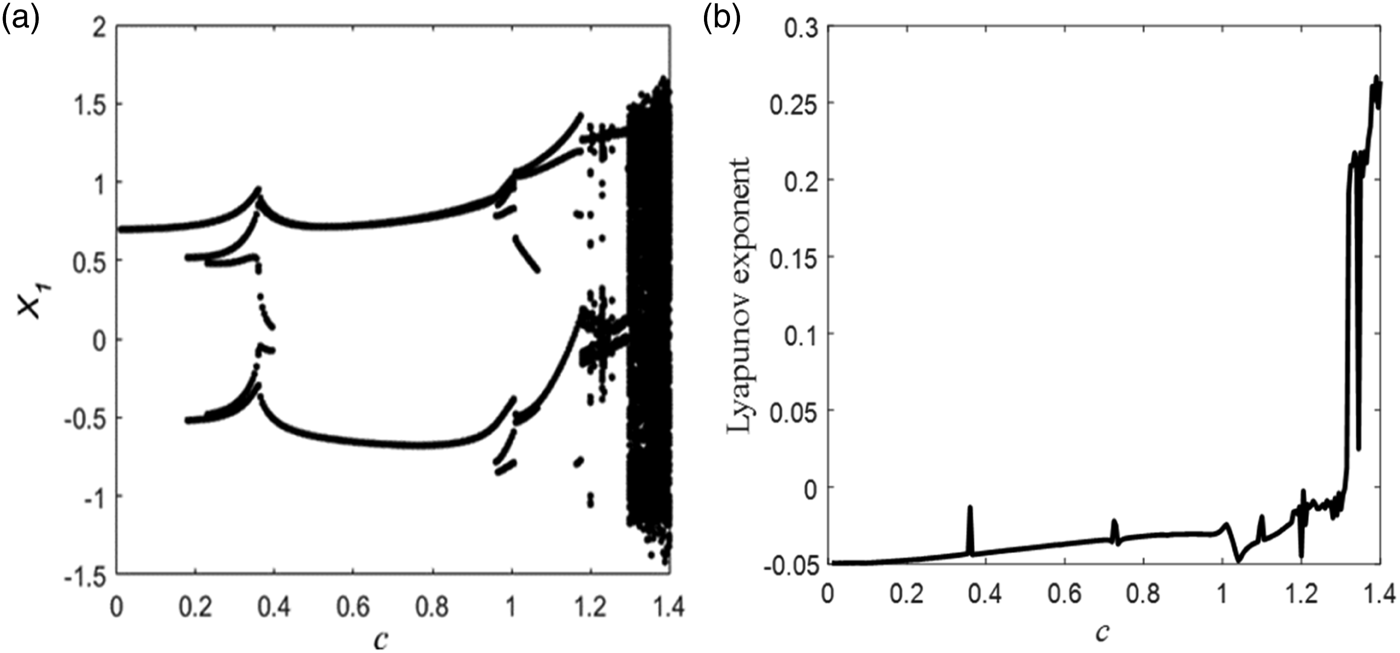

Figures 3, 4 and 5 are the time histories(a), phase-plane portraits(b) and Poincare maps (c) at different velocities.

Figure 3.

c = 0.79.

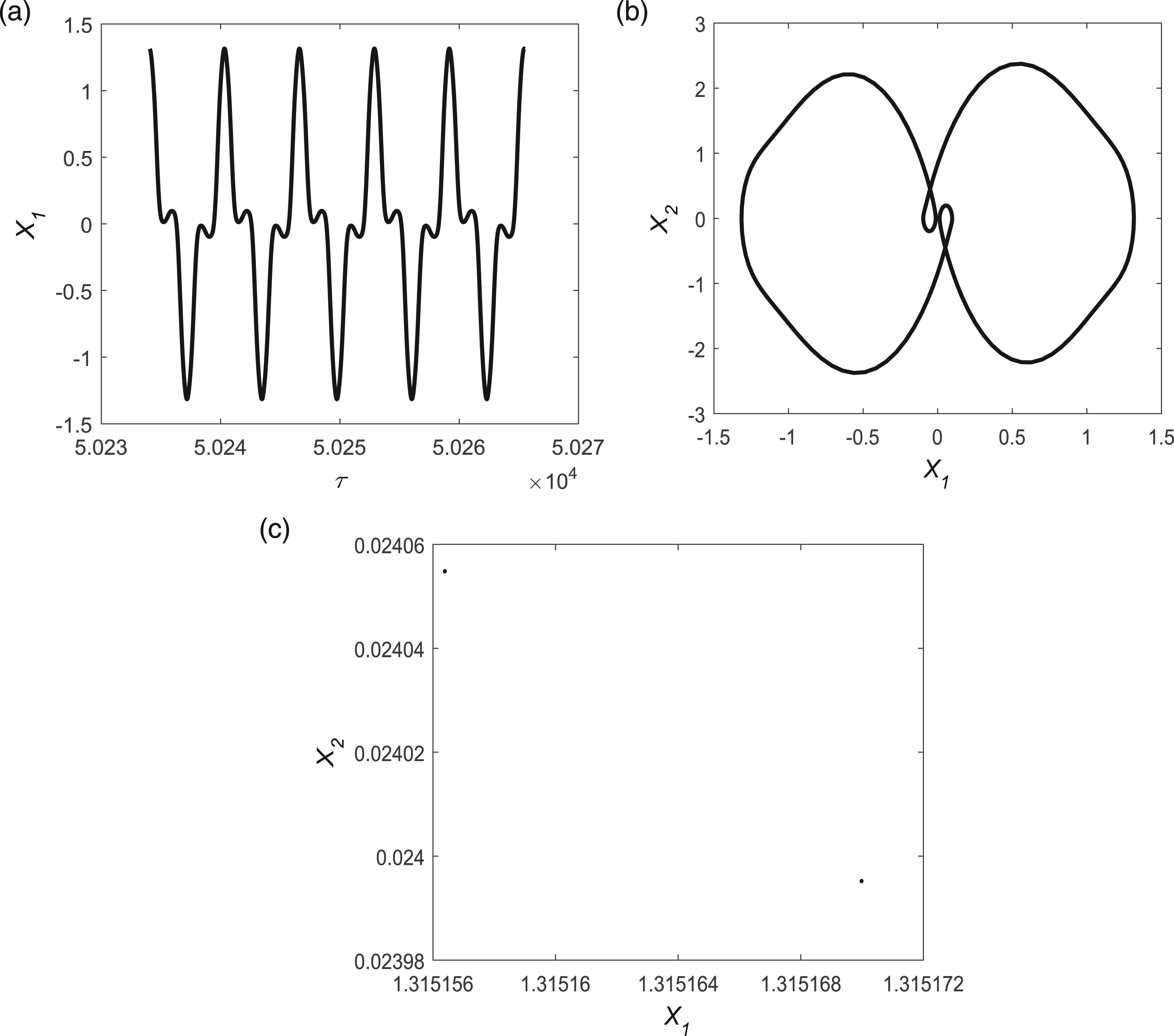
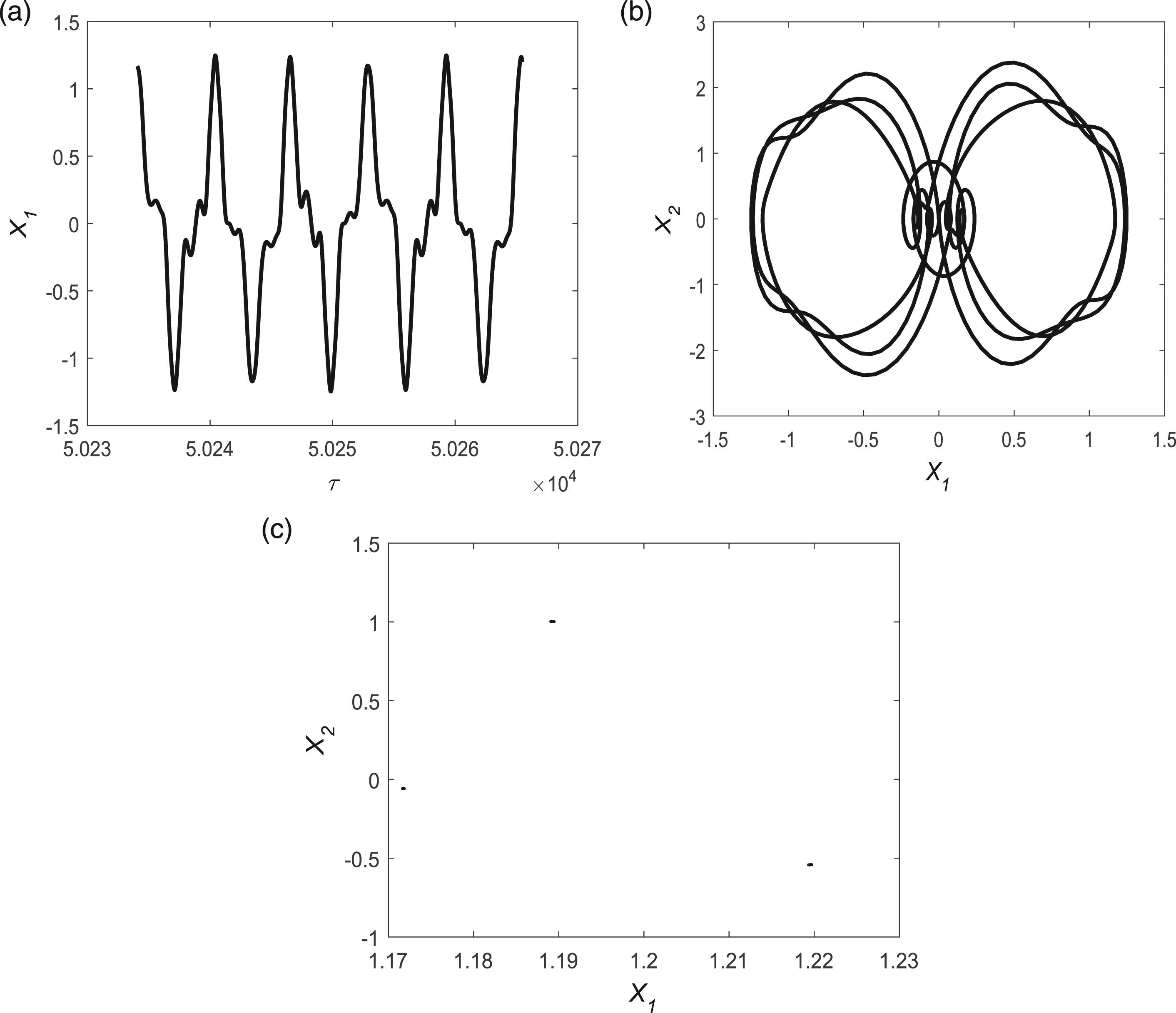
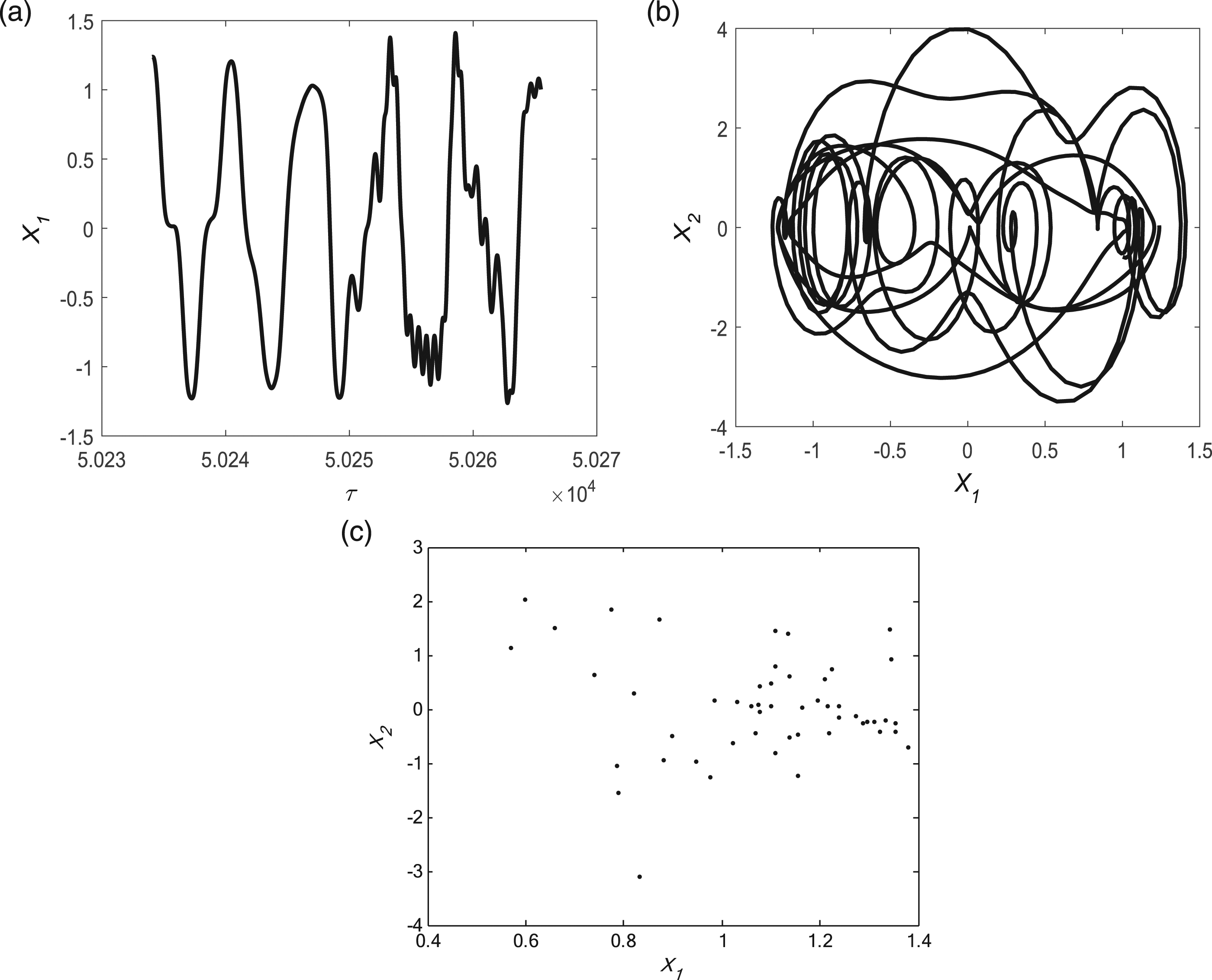
Figure 4.

c = 1.23.

Figure 5.

c = 1.32.

As shown in Figure 3, when c = 0.79, the phase-plane portraits exhibit many closed figures, and two fixed points in the Poincaré map suggest that the membrane is in a state of period-2 motion. As shown in Figure 4, when c = 1.23, there is a closed curve in the phase-plane portraits, and a few discrete points in the Poincaré map reveals the membrane is in a period-doubling motion. As shown in Figure 5, when c = 1.32, the phase-plane portraits are unclosed curves, and a dense point in the Poincaré map demonstrates that the membrane is chaotic.

As shown in Figure 6, other given parameters remain unchanged and the orthotropic coefficient e is changed to 2. The bifurcation graph and largest Lyapunov exponent of the membrane system are given to identify the global dynamical behaviours.

Figure 6.

(a) The bifurcation graph; (b) Largest Lyapunov exponent.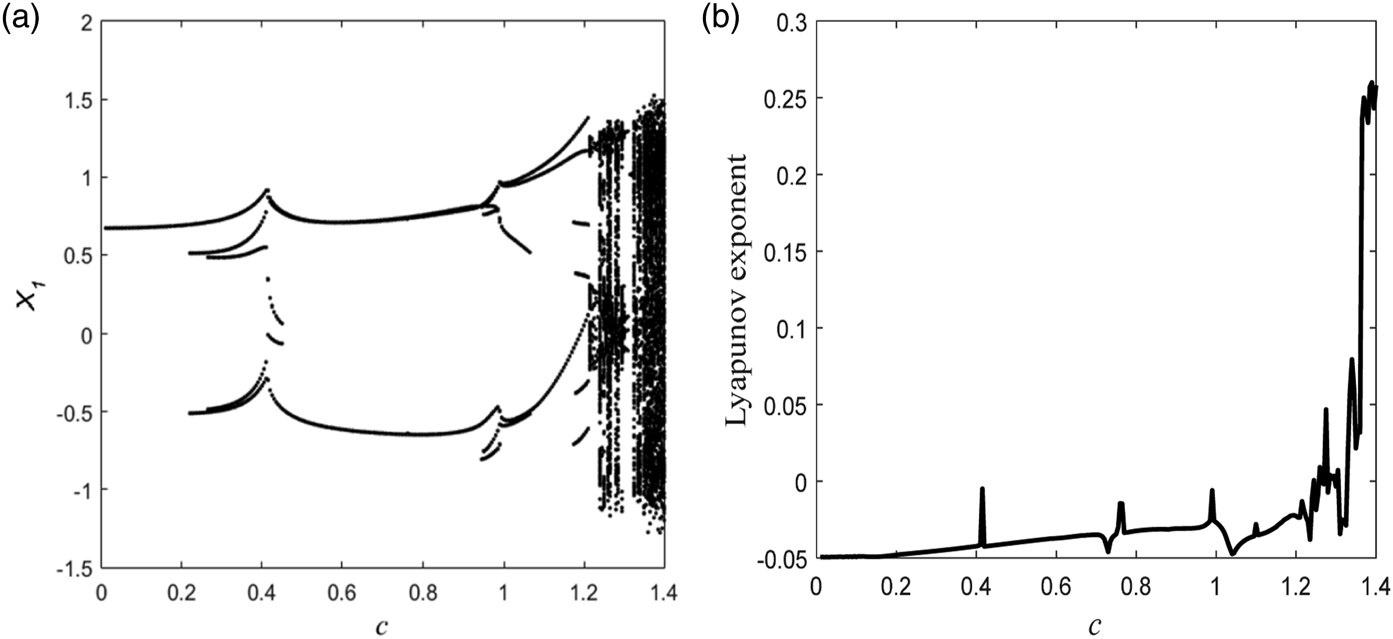

Comparing Figure 2 with Figure 6, it can be seen that the orthotropic coefficient is different, and the area generated by the periodic and chaotic motion of the membrane is also different. The motion of the membrane changes from periodic motion to chaotic motion with increasing the velocity. This indicates that different initial parameters will have a significant influence on the dynamic behaviours.

The influence of the aspect ratio on the nonlinear dynamics

Taking as the bifurcation parameter, a membrane system is considered with the orthotropic coefficient e = 1.2, the velocity c = 0.5 and the aspect ratio r is the bifurcation parameter. The bifurcation graph and largest Lyapunov exponent are presented to identify the global dynamic behaviours.

As shown in the Figure 7, when the aspect ratio is 0.2 ≤ r ≤ 0.26, there is a dense spot on the bifurcation graph, indicating that the membrane in this area is chaotic. Meanwhile, the largest Lyapunov exponent is positive. When the aspect ratio is 0.26 < r ≤ 2, a point in the bifurcation graph signifies that the system is in periodic motion. Meanwhile, the largest Lyapunov exponent is negative. It is apparent from these figures that the system is more stable with a larger aspect ratio.

Figure 7.

(a) The bifurcation graph; (b) Largest Lyapunov exponent.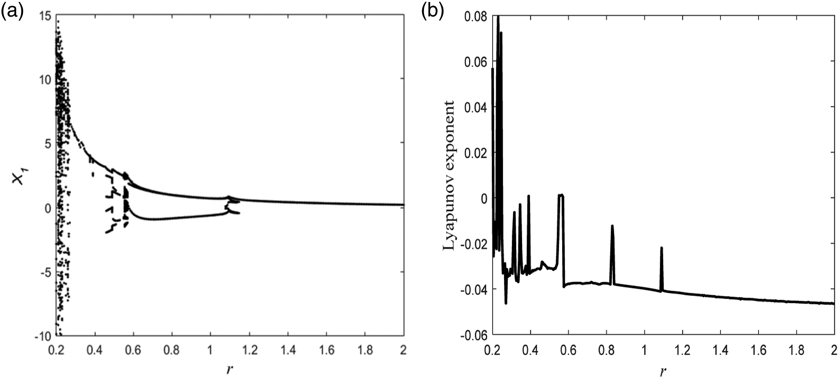

The influence of the orthotropic coefficient on the nonlinear dynamics

Taking the orthotropic coefficient e as the bifurcation parameter, a membrane system is considered with velocity c = 0.5 and aspect ratio r = 1. The bifurcation graph and largest Lyapunov exponent of the membrane are plotted to identify the global dynamic behaviours.

In Figure 8, the orthotropic coefficient interval is 1.11 ≤ e ≤ 3, and a few discrete points in the bifurcation graph illustrate that the system is in periodic motion. Meanwhile, the largest Lyapunov exponent is always negative.

Figure 8.

(a) The bifurcation graph; (b) Largest Lyapunov exponent.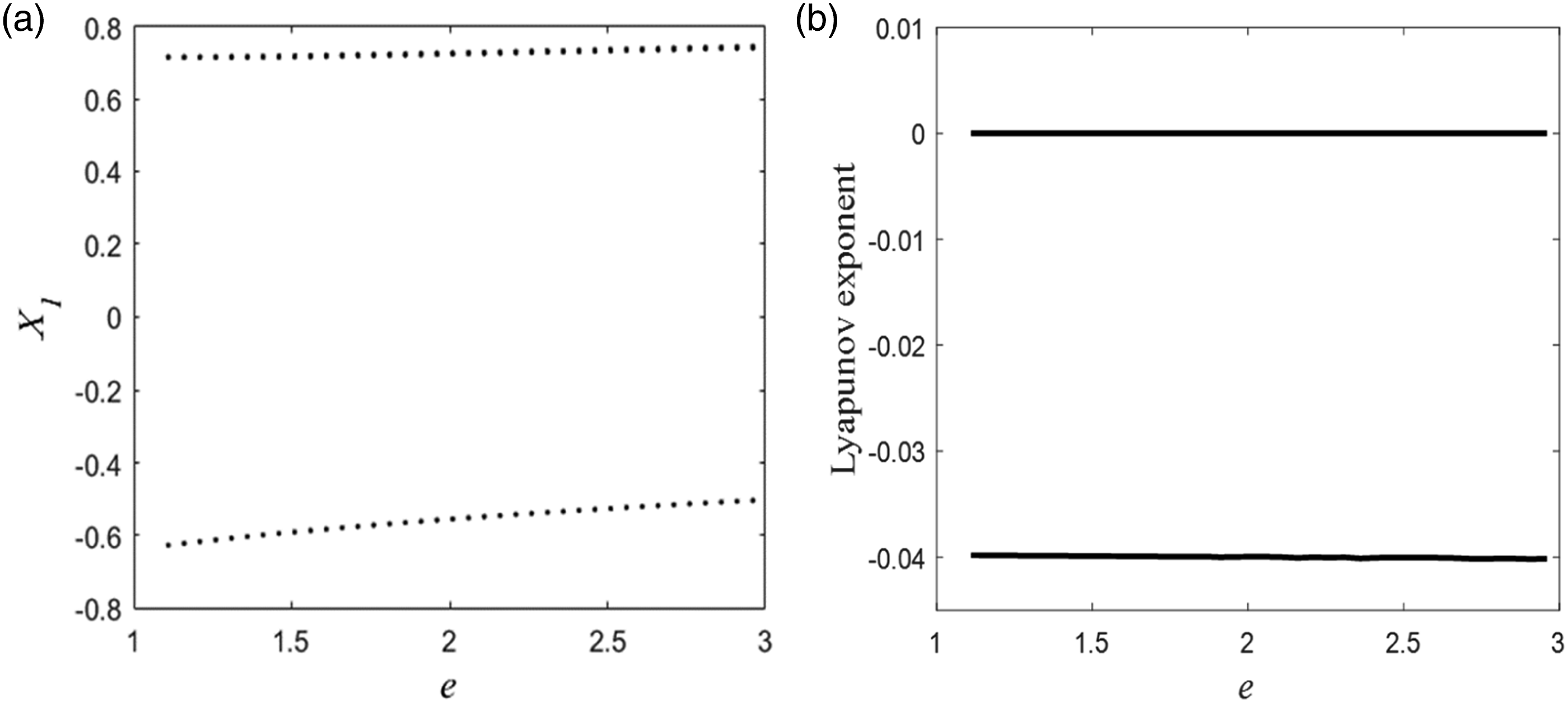

Conclusion

This paper addresses the dynamic behaviours of an orthotropic moving membrane. Considering the material properties of the membrane, a mathematical model is developed via von Karman’s large deflection theory. The dynamic behaviours are demonstrated by numerical analysis based on the Runge–Kutta fourth-order method. These numerical examples illustrate the influences of the velocity, aspect ratio, and orthotropic coefficient on the nonlinear dynamics of the orthotropic membrane.

(1) When 0.01 ≤ c < 1.3, a few discrete points in the bifurcation graph imply that the system is in periodic motion. Meanwhile, the largest Lyapunov exponent is negative. When 1.3 ≤ c ≤ 1.4, there is a dense spot on the bifurcation graph, indicating that the membrane in this area is in chaotic motion. Meanwhile, the largest Lyapunov exponent is positive. This proves that the greater the velocity of the membrane, the easier it is to diverge and lose stability.

(2) When the aspect ratio is 0.2 ≤ r ≤ 0.26, there is a dense spot on the bifurcation graph, indicating that the membrane in this area is chaotic. Meanwhile, the largest Lyapunov exponent is positive. When the aspect ratio is 0.26 < r ≤ 2, a point in the bifurcation graph denotes that the system is in periodic motion. Meanwhile, the largest Lyapunov exponent is negative. It is apparent from these figures that the system is more stable with a larger aspect ratio.

(3) When the orthotropic coefficient interval is 1.11 ≤ e ≤ 3, a few discrete points in the bifurcation graph demonstrate that the system is in periodic motion. Meanwhile, the largest Lyapunov exponent is always negative.

(4) As the velocity and aspect ratio change, the system exhibits period-doubling motion and chaotic motion. Therefore, the printing speed should be reasonably selected to improve the stability of the membrane and the printing accuracy, and the aspect ratio of the membrane should be increased appropriately to avoid the occurrence of chaos.

To sum up, this paper mainly focuses on the nonlinear vibration of the orthotropic moving membrane. Additionally, the nanostructured membrane also has good prospects for practical engineering, and its fabrication mechanism has been clearly demonstrated in.Refs [26,27]. Further investigation on the nonlinear vibration of nanostructured membranes would be a major advancement.