Fault diagnosis of rolling bearing based on singular spectrum analysis and wide convolution kernel neural network

Abstract

Research on bearing fault diagnosis generally uses a single signal processing method to extract features to a certain extent and then empirically judges the fault type at this stage. However, this approach has a poor fault feature extraction effect when the noise interference signal is large and subjective human errors. The diagnosis effect is determined by external interference and has no practical value. This paper proposes a rolling bearing fault diagnosis method based on singular spectrum analysis and a wide convolution kernel neural network, which can effectively extract the fault features of the rolling bearing crack fault signal with a strong noise interference and realize the efficient diagnosis of this kind of fault. Gaussian white noise is added to the standard bearing fault signal to construct the vibration signal with noise interference. Then, the noisy one-dimensional time series signal is preprocessed, including the data division into the training and test sets and the different kinds of numbering processing. Singular spectrum analysis is performed on the preprocessed data. Then, the denoised training set is used as input in a deep convolution neural network with a wide convolution kernel for feature extraction and model training. The trained diagnosis model is used for the fault prediction of the next test set, and the relevant diagnosis results are output. The test results show that this method can ensure the overall accuracy of more than 90% under the background of high noise, and the diagnosis rate of the model under various working conditions is stably maintained at more than 93%, without the collapse of diagnosis stability under the sudden change of noise. The advantages of model diagnosis efficiency and structural improvement fit are prominent.

Introduction

As one of the key parts of a rotating machinery, the rolling bearing’s health condition affects the normal operation of the entire rotating machinery system. The timely detection of bearing fault can effectively reduce production loss. At present, rolling bearing fault can be diagnosed by vibration signal feature extraction; especially with the development of deep learning, intelligent diagnosis methods combined with deep learning have achieved remarkable results. Gan ¹ proposed a hierarchical diagnosis network structure based on deep learning, which can effectively identify the fault mode of rolling bearing. He ² described the relevant principles and summarized the methods of in-depth learning that can be used for bearing fault diagnosis. Jia ³ proposed deep normalized convolution neural network to complete the classification of mechanical unbalanced faults and visually analyze the fault characteristics. Khan ⁴ applied deep learning to system health management, and introduced the principle and structure of the method. Zhao ⁵ applied relevant deep learning algorithm to machine health monitoring. The research objects are mainly pure fault signals. However, the fault feature components in the signal, especially the early weak fault features, are easily concealed by noise and other irrelevant signal components, preventing the timely detection of equipment fault. ⁶ Therefore, using the signal decomposition method to decompose the vibration signal into a series of sub signal components with a clear physical meaning and then extracting fault feature components from them is particularly important for mechanical fault diagnosis. ⁷

The methods of signal decomposition can be divided into decomposition in the time domain, frequency domain filtering method, time-frequency domain reconstruction method, and subspace decomposition method. Decomposition in the time domain, such as empirical mode decomposition (EMD), can decompose the vibration signals containing multiple components into several single mode intrinsic mode functions (IMFs). The feature can be extracted by component morphology analysis but will be subjected to noise interference because of its physical meaning. Frequency domain filtering methods, such as wavelet transform, can analyze the high and low frequency components of non-stationary signals and extract features, but this method has only one kind of basis function, which cannot match all the components of the signal and lacks adaptability. Time-frequency reconstruction methods, such as short-time Fourier transform (FT), choose different window functions to make the signal locally stationary in the time-frequency domain and can analyze the power spectrum of the signal but have difficulty balancing the optimal form of resolution between the time-frequency and non-stationary signals with large fluctuations. Subspace decomposition methods, such as singular value decomposition (SVD), can decompose signals according to a singular value and extract the main signal components according to the singular value. These methods have an excellent effect on noise reduction and can improve the signal-to-noise ratio (SNR), but their function is relatively limited, requiring them to cooperate with other methods in the overall analysis.

On the basis of the research results at this stage, some shortcomings are difficult to compensate for, including the accuracy of the selection of effective original signal components and the limitations of the application, which often lead to fuzzy final signal features and inaccurate diagnosis. Cong et al. ⁸ introduced short-time matrix sequence and singular value ratio into vibration signal processing, thereby detecting early faults well. However, due to noise signal interference, the envelope analysis of the original signal cannot detect faults. Wang et al. ⁹ used the manifold learning algorithm to adaptively fuse fault related modes with different noises to retain the real fault related transients and suppress the components irrelevant to faults, thus obtaining a good denoising effect, but the denoising effect of high noise was not verified. The ensemble EMD (EEMD), ¹⁰ which is an improvement of EMD, is also used in the noise reduction of fault signals. Han et al. ¹¹ combined the EEMD method with the block threshold strategy to denoise vibration signals and achieved relatively good experimental results. However, the reconstructed signal deviates greatly from the clean signal, and the application range is limited to small noise.

To meet the noise reduction requirements of bearing fault signals, SVD is selected as the main body of the singular spectrum analysis method. On this basis, combined with the relevant self-learning diagnosis classification system, the machine or deep learning method is introduced to meet the effect of big data intelligent diagnosis. Currently, the commonly used methods of deep learning include auto encoders (AEs), convolutional neural network (CNN), and wide convolution depth neural network (WDCNN). AE is an artificial neural network with a multi-layer encoding and decoding operation to complete unsupervised learning of features and a very good ability to extract data features, but it is not flexible enough to be applied in multiple scenes. CNN, including convolution calculation and feedforward neural network with a deep structure, achieves feature depth extraction through repeated convolution and downsampling operation. CNN has a deep structure and a highly accurate final learning classification, but the classification efficiency is low when the structure parameters must be continuously optimized and too many samples are used. WDCNN optimizes the convolution kernel size based on CNN and deepens the network structure. WDCNN realizes large sampling, has a high efficiency, and does not lose extremely large features, but its final classification accuracy is slightly reduced.

Combined with the above characteristics, a fault diagnosis model of rolling bearing based on singular spectrum analysis (SSA) and a one-dimensional wide convolution kernel neural network is proposed in this paper. Through the comparison with denoising AE and EMD, the accuracy and anti-interference of the proposed method are verified. The rest of this paper is organized as follows. In the Description of Theory and Method section, the structure of the one-dimensional CNN, the SSA method, and the algorithm flow are described. In the Establish the Diagnosis Model section, the construction method of the diagnosis model and the relevant dimension parameters are introduced. In the Simulation Test and Analysis method, the noise reduction and diagnosis effects based on the SSA-WDCNN method are obtained through simulation and comparative experiments. The Conclusion section presents the conclusion.

Description of theory and method

This section mainly introduces the theoretical basis of the proposed method, including the structure of the one-dimensional CNN and the SSA method.

Singular spectrum analysis

Singular spectrum analysis is used to decompose and denoise bearing noise fault signals. Compared with the common signal processing methods, such as Fourier transform (FT), wavelet decomposition, EMD, and variational mode decomposition, can complete the relevant signal denoising decomposition and feature extraction to a certain extent as well, but the effect will be very poor under the interference of large noise and the main signal separation will be difficult to achieve, especially for the bearing noise. The discrimination of signal components lacks clarity. SVD can separate and identify multi-component signals through singular values, especially in the case of complex noise reduction and feature extraction.

Singular spectrum analysis can decompose a one-dimensional time series matrix into a corresponding singular value spectrum according to its eigenvalues and eigenvectors. The components of the time series represented by different singular values vary. The multi-component independent information obtained from the decomposition includes the principal component and noise. SSA is a nonparametric decomposition technique, which can effectively extract the main components of sequence information. SSA includes two stages, namely, decomposition and reconstruction, which can be further divided into four steps: embedding, SVD, reconstruction, and diagonal averaging. ¹²

(1) Embedding. The noise vibration time sequence signal is recorded as $X_N=\left\{f_1,f_2\cdots f_N\right\}$ and then transformed into trajectory matrix $X$ :

$$X=\left(\begin{array}{ccc}{f}_1& \cdots & f_n\\ ⋮& \ddots & ⋮\\ f_m& \cdots & f_{n+m-1}\end{array}\right)$$

(1)

m is the embedding dimension, which is determined by the rank of the trajectory matrix; N is the length of the timing signal in one dimension, and n is a constant, which is determined by N and m. In the equation, $2\le m\le N\mathrm{∕}2$ , $n=N-m+1$ .

• (2) SVD. The noise reduction effect of SVD often depends on the selection of the number of singular values. ¹³ Let covariance matrix $C=X{X}^T$ . Then, $m$ eigenvalues of matrix $C$ are obtained: $\hspace{1em}{\lambda }_1\ge {\lambda }_2\ge \dots \ge {\lambda }_m\ge 0$ . The corresponding eigenvector is $\hspace{1em}{U}_1\mathrm{,}{U}_2\cdots U_m$ , $V_i=X^T{U}_i\mathrm{∕}\sqrt{{\lambda }_i}\left(\text{i}=1,\cdots m\right)$ , where $U_i$ and $V_i$ are the left and right singular vectors of matrix $X$ , and $m$ is the rank of matrix $X$ , which is equal to the embedding dimension. Thus, trajectory matrix $X$ can be written as follows

$$X=X_1+X_2+\cdots X_i+\cdots X_m$$

(2)

$$X_i=\sqrt{{\lambda }_i}{U}_i{V}_i^T$$

(3)

• (3) Reconstruction. First, the order of singular value to be extracted is set as $d\hspace{1em}\left(d\hspace{1em}<\hspace{1em}m\right)$ . Only the components of the SVD from the first order to the $d$ order can be obtained, and the singular value components of other orders are set to zero. Then, the first several order singular value components are selected from the d-order singular value components for reconstruction. The specific order can be determined by the specific noise reduction effect, and a new singular value matrix is obtained. Meanwhile, we can obtain a new trajectory matrix $\left(Y\right)$ for combination with $X_i=\sqrt{{\lambda }_i}{U}_i{V}_i^T\left(\text{i}=1\cdots d\right)$ .

$$Y=X_1+\dots +X_i$$

(4)

• (4) Diagonal averaging. In this operation, the diagonal elements of each submatrix are averaged as a one-dimensional sequence with corresponding length $N$ , so that the length of the new trajectory matrix $Y$ is $N$ . Let $Y$ be an $m\times n$ matrix, where $m\le n$ and $N=m+n-1$ . Diagonal averaging can transform $Y$ into a one-dimensional time series.

The reconstructed one-dimensional time series is $Y=\left\{y_1,y_2,\cdots y_k\cdots y_N\right\}$ .

$$y_k=\{\begin{array}{c}\frac{1}{k}{\displaystyle \sum _{p=1}^k{y}_{P\mathrm{,}k-p+1}^{\ast }}\left(1\le k<m\right)\\ \frac{1}{m}{\displaystyle \sum _{P=1}^m{y}_{P\mathrm{,}k-p+1}^{\ast }}\left(m\le k<n\right)\\ \frac{1}{N-k+1}{\displaystyle \sum _{P=k-n+1}^m{y}_{P\mathrm{,}k-p+1}^{\ast }}\left(n\le k<N\right)\end{array}$$

(5)

Wide deep convolution kernel neural network

After the signal decomposition and noise reduction operation, the deep learning method is used to learn and diagnose the relevant fault features. Combined with the number of samples and the demand of diagnosis, parameter improvement and structure optimization based on conventional wide convolution kernel neural networks are advantageous for the subsequent diagnosis.

A typical CNN is composed of convolution, pooling, and full connection layers. The convolution kernel is used as the feature extractor of the convolution layer, which can be divided into two dimensions. In this study, one-dimensional convolution is used for the feature extraction of the time series signal. The pooling layer is a subsampling layer and selects features, reduces the number of features, reduces the amount of calculation, and effectively prevents the over fitting of the model. The full connection layer and other layers mainly realize the function of feature sharing and classification and finally carry out relevant fault diagnosis.

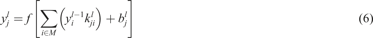
The one-dimensional CNN uses a one-dimensional array as the convolution core, and the forward propagation output of the convolution operation is as follows

$$y_j^l=f\left[{\displaystyle \sum _{i\in M}\left(y_i^{l-1}{k}_{ji}^l\right)+b_j^l}\right]$$

(6)

where $y_j^l$ is the weight of the j-neuron output in layer $l$ , $y_i^{l-1}$ is the weight of the j-neuron output in layer $l-1$ , $M$ is the convolution kernel width, $k_{ji}^l$ is the convolution nucleus from the i-neuron of layer $l-1$ to the j-neuron of layer $l$ , ${\displaystyle \sum _{i\in M}\left(y_i^{l-1}{k}_{ji}^l\right)}$ is the mapping of the entire input feature, $b_j^l$ is the weight deviation of the j-neuron in layer $l$ , and $f$ is the activation function of the convolution layer. We use rectified linear unit (RELU) ¹⁴ as the modified linear unit function.

The pooling layer performs the downsampling operation, and the commonly used pooling functions include average pooling and max pooling. ¹⁵ The maximum pooling function is used for downsampling.

$$y_i^l=\max pooling\left(x_i^{1-1},scale,stride\right)$$

(7)

where $y_i^l$ is the weight of the j-neuron output in the first layer, $maxpooling$ is the maximum pooling function, $scale$ is the pooling width, and $stride$ is the pooling step.

In the fully connected layer, the output of the last pooling layer is expanded and flattened into one-dimensional feature vectors. Finally, the softmax function is used to classify the features.

$$q^j=softmax\left(z^{\left(l+1\right)j}\right)$$

(8)

where $q^j$ is the characteristic category of the j-neuron output, $softmax$ is the activation function, and $z^{\left(l+1\right)j}$ is the weight of the j-neuron output in layer $l+1$ .

SSA-WDCNN algorithm flow and characteristics

In this study, a bearing fault diagnosis model based on SSA and the WDCNN algorithm is adopted. The algorithm flow is shown in Figure 1. SSA, as the main way of reducing the noise of the bearing vibration signal, can effectively extract the correlation components of the original signal and amplify the features and is coupled with an improved wide CNNs to carry out further self-filtering learning and the feature extraction operation on the follow-up signals to complete the bearing fault diagnosis. The algorithm flow is as follows:

Figure 1.

Algorithm flow.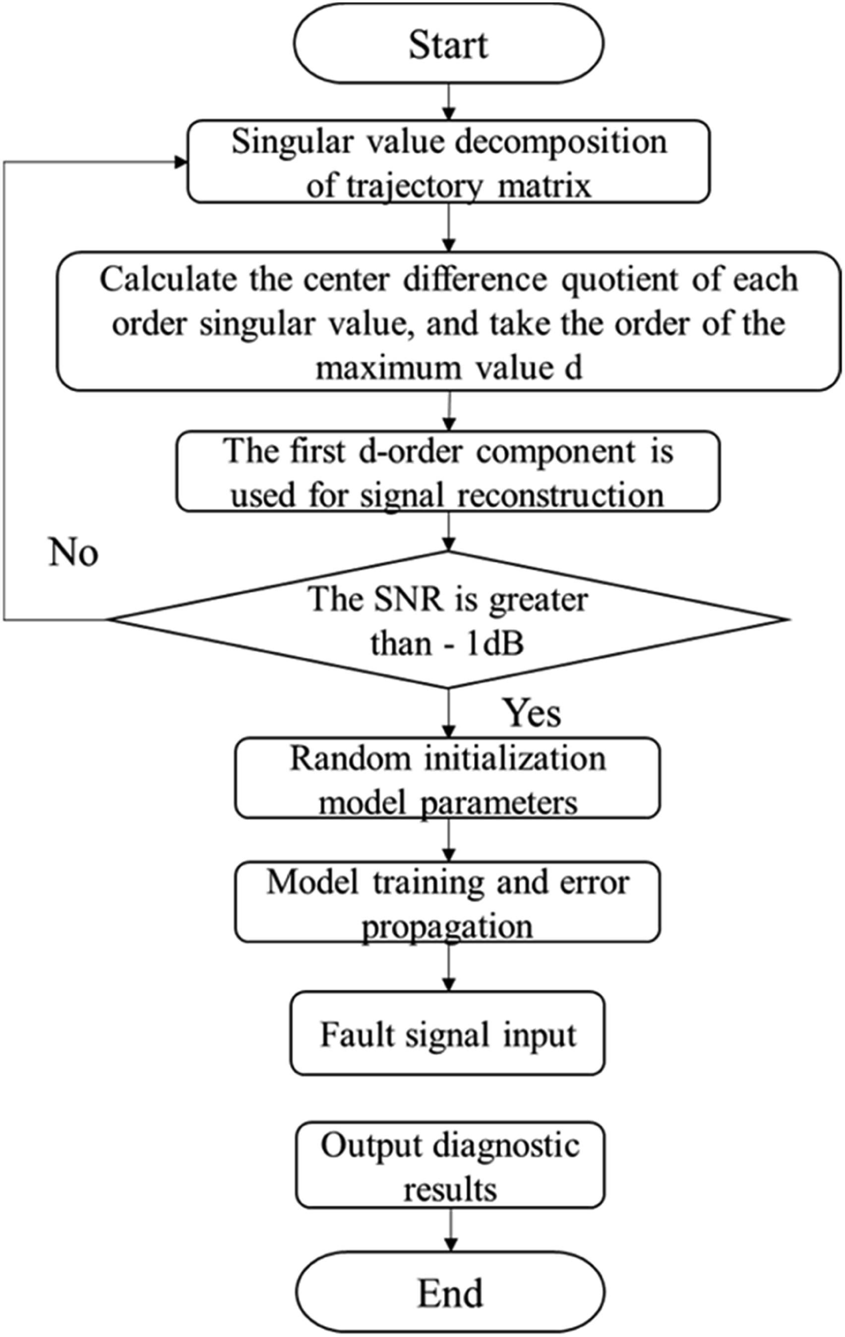

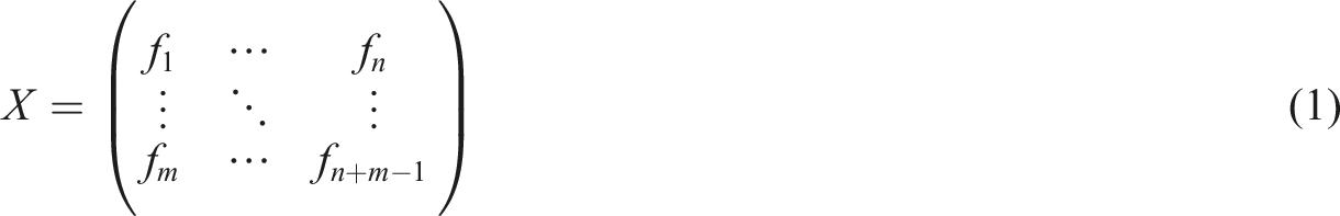
Step 1

Select the appropriate window length and arrange the noisy signals with time delay to obtain Hankel (Trajectory) matrix X.

Step 2

Decompose the trajectory matrix through SVD and matrix X into the form shown in equations (2) and (3).

Step 3

Divide the m components of the trajectory matrix into d disjoint groups, which represent different trend components. Select the effective singular value components using the method of two-thirds mean of singular value and obtain a new trajectory matrix $Y=X_1+\dots +X_i$ .

Step 4

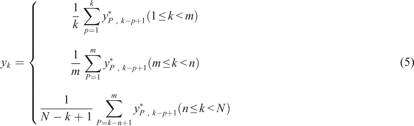
Reconstruct the signal by using the time empirical orthogonal function equation (5) and the time principal component, where $y_{P\mathrm{,}k-p+1}^{\ast }$ reflects the weight of $y_k$ in the original time series. The one-dimensional time series processed by SVD is $Y=\left\{y_1,y_2,\cdots y_k\cdots y_N\right\}$ .

Step 5

Initialize the parameter of the one-dimensional CNN. Use timing signal Y as the input and select the length for the sample overlap operation.

Step 6

Wide convolution kernels extract features efficiently, while small convolution kernels expand the depth of the entire network. Process signal $x$ by batch normalization (BN) and obtain signal $\widehat{x}=\frac{x-x_{\text{min}}}{x_{\text{max}}-x_{\text{min}}}$ to increase the generalization ability.

Step 7

Calculate the derivative value of the objective function about the ownership value layer by layer from the back to the front and use error back propagation to optimize the weight distribution of the neural network by using the chain rule.

Step 8

Complete the feature comparison through neural network self-learning and output the bearing fault diagnosis results.

The characteristics of the model based on SSA-WDCNN are as follows:

(1) In view of the limitation of common signal processing methods in filtering noisy signals and the relatively fuzzy fault features after processing, the SSA signal processing method can filter noisy signals more effectively and select relevant components of the original signal for reconstruction more accurately, exhibiting better noise reduction stability and feature amplification effect.

(2) Wide CNNs can achieve double signal processing, and the self-convolution operation further filters the interference during feature extraction. The combination of a multi-layer network with BN processing can deepen the generalization ability of the entire model. Optimizing the weights of neural networks by self-training can ensure the accuracy of model classification. Overall, the whole high efficiency and intelligent fault diagnosis mode is realized.

(3) The combination of signal processing with deep learning can eliminate the interference of external environment to the greatest extent. Meanwhile, the deep neural network can operate in multi-working conditions or a multi-interferences scene and complete efficient fault identification without feature distortion, which has a high practical value.

Establish the diagnosis model

This section mainly introduces the data processing in model construction and the specific setting of relevant parameter size.

Data preprocessing

In this study, the training and test data were obtained from the rolling bearing data center of Case Western Reserve University. ¹⁶ The test object is the drive end bearing, the model is deep groove ball bearing skf6205, the crack fault is made by electrical discharge machining, and the sampling frequency is 12 kHz. According to the location and diameter of the bearing crack, the entire data is divided into nine fault types and one normal bearing health condition. The nine faults include the following: 0.007-in rolling element (B007), 0.014-in rolling element (B014), 0.021-in rolling element (B021), 0.007-in inner ring (IR007), 0.014-in inner ring (IR014), 0.021-in inner ring (IR021), 0.007-in outer ring (OR007), 0.014-in outer ring (OR014), and 0.021-in outer ring (OR021).

Meanwhile, four data sets were prepared for different working conditions, including 0 HP (1797 rpm), 1 HP (1772 rpm), 2 HP (1750 rpm), and 3 HP (1730 rpm). Each test set contains 7000 training samples and 1000 test samples. The length of each sample signal is 2048, and each signal segment must be normalized before training. In this paper, min-max normalization is used to normalize signal $x$ .

$$\widehat{x}=\frac{x-x_{\text{min}}}{x_{\text{max}}-x_{\text{min}}}$$

(9)

To improve the generalization ability of model learning, the training samples can be appropriately increased, that is, the generalization of the entire neural network can be increased through the data set enhancement technology. In this study, the sample overlap method is used to enhance the data set. The length of each training sample is 2048, and the amount of overlap is 28. The enhanced training samples can satisfy the training needs of the entire neural network.

Parameter setting and model design of WDCNN

To improve the feature extraction ability of the diagnosis model, a deep CNN with a wide convolution kernel is used as the feature extraction part of the entire model. The structure of the entire model is shown in Figure 2.

Figure 2.

Network framework of wide convolution depth neural network.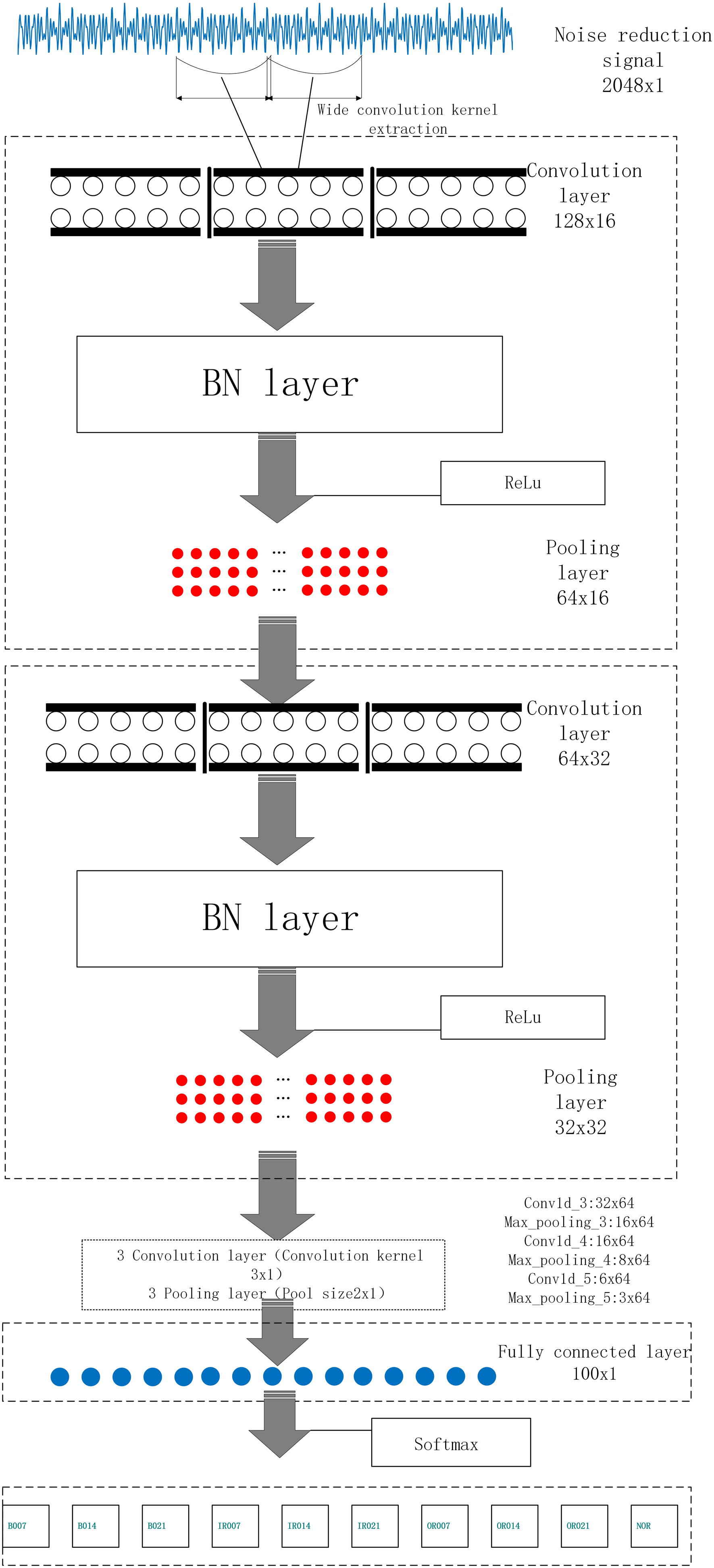

BN layer optimization

The first convolution layer of the model uses a large-scale wide convolution kernel, which can realize the short-term feature extraction of the signal, extract the effective fault feature of the original signal to the greatest extent, and discard the other relatively invalid features, significantly improving the training efficiency of the entire network. In addition to the first convolution layer, the convolution cores of the other convolution layers are small-scale to construct the depth of the neural network and prevent over fitting. Meanwhile, BN ¹⁷ is performed between the convolution and pooling layers, which can limit the output value of the upper layer within a small interval, resulting in the normal distribution of data, and the activated input value falls in the input sensitive area of the nonlinear function, which can improve the network training efficiency and enhance the generalization ability. ¹⁸

A small batch set with $K$ samples is provided, and the net input of the layer is $z^{\left(1\mathrm{,}l\right)}\mathrm{,}\cdots \mathrm{,}{z}^{\left(K\mathrm{,}l\right)}$ , and the neuron output is $a^{\left(l\right)}$

$${\mu }_B=\frac{1}{K}{\displaystyle \sum _{k=1}^K{z}^{\left(k,l\right)}}$$

(10)

$${\sigma }_B^2=\frac{1}{K}{\displaystyle \sum _{k-=1}^K\left(z^{\left(k,l\right)}-{\mu }_B\right)\cdot \left(z^{\left(k,l\right)}-{\mu }_B\right)}$$

(11)

$${\widehat{z}}^{\left(l\right)}=\frac{z^{\left(l\right)}-{\mu }_B}{\sqrt{{\sigma }_B^2+\mathit{ϵ}}}\cdot {\gamma }^{\left(l\right)}+{\beta }^{\left(l\right)}$$

(12)

$$a^{\left(l\right)}=f\left(B{N}_{\gamma ,\beta }\left({\widehat{z}}^{\left(l\right)}\right)\right)$$

(13)

where ${\mu }_B$ is the mean value of the net input, ${\sigma }_B^2$ is the variance of the net input, ${\widehat{z}}^{\left(l\right)}$ is the net input for the standard normal output, ${\gamma }^{\left(l\right)}$ is the BN layer scaling parameter vector, ${\beta }^{\left(l\right)}$ is the BN layer translation parameter vector, $\mathit{ϵ}$ is the constant term for maintaining numerical stability, and $f(\cdot )$ is the BN layer activation function.

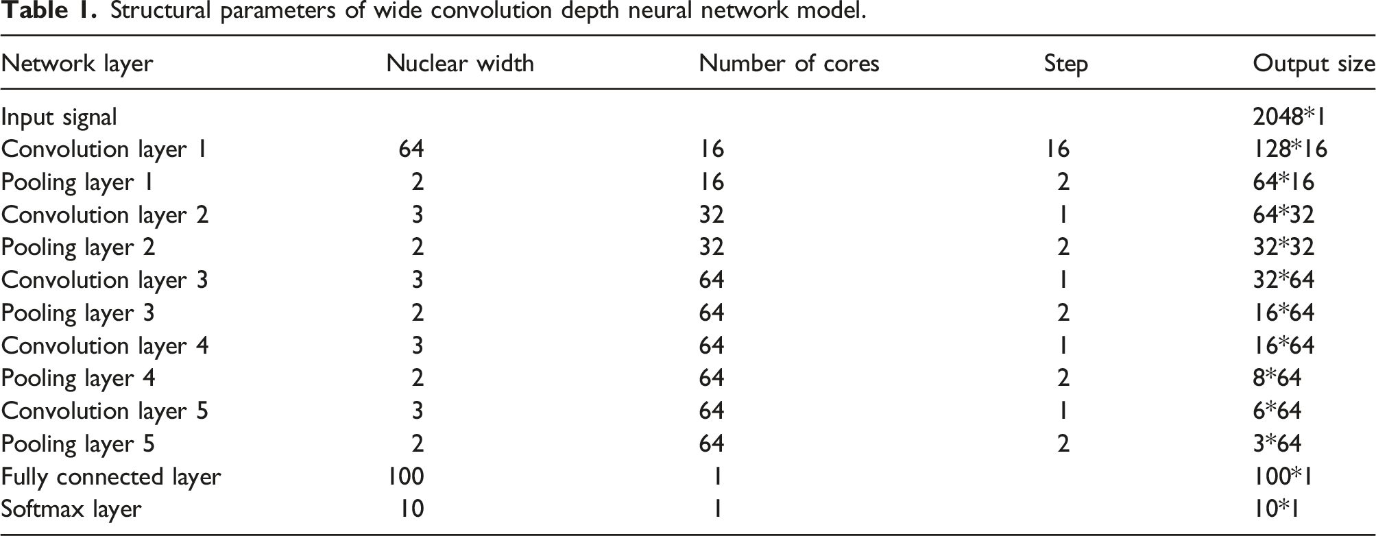
Structural parameters of WDCNN model

The structural parameters of the entire CNN are shown in Table 1.

Table 1.

Structural parameters of wide convolution depth neural network model.

Network layer	Nuclear width	Number of cores	Step	Output size
Input signal				2048*1
Convolution layer 1	64	16	16	128*16
Pooling layer 1	2	16	2	64*16
Convolution layer 2	3	32	1	64*32
Pooling layer 2	2	32	2	32*32
Convolution layer 3	3	64	1	32*64
Pooling layer 3	2	64	2	16*64
Convolution layer 4	3	64	1	16*64
Pooling layer 4	2	64	2	8*64
Convolution layer 5	3	64	1	6*64
Pooling layer 5	2	64	2	3*64
Fully connected layer	100	1		100*1
Softmax layer	10	1		10*1

The vibration signal after singular spectrum denoising is first extracted from the wide convolution check signal of the first convolution layer for short-term feature extraction, and the obtained feature is normalized in batches, so that the standard normal distribution of the feature falls in the sensitive area of the activation function. ¹⁸ Then, the RELU function is activated to transform the convolution output feature nonlinearly to realize the next level mapping. Subsequently, the feature is downsampled in the pooling layer, and five layers of convolution and pooling are performed alternately. Finally, 10 kinds of faults are used as input and processed by softmax. In the convolution, zero padding is used to ensure the same size before and after convolution. In the optimization of the super parameters of the entire network model, the Adam (adaptive motions) optimization algorithm is used, ¹⁹ which can adaptively adjust the learning rate and improve the robustness of the selection of super parameters of the entire model.

Simulation test and analysis

The CNN is built using the Python tensorflow framework. The specific test includes comparing and verifying the noise reduction effect of SSA and the diagnostic accuracy of the proposed diagnostic model and setting different test conditions to test the anti-interference and generalization ability of the model.

Analysis of noise reduction effect based on SSA

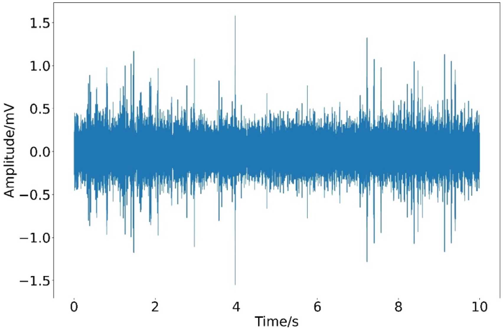
In this study, Gaussian white noise is added to the original bearing vibration signal to obtain a mixed signal with noise. Taking the B014 fault signal in data set 0 HP as an example, the white noise with SNR ²⁰ = −10 dB is added. The effect is shown in Figure 3.

Figure 3.

Time domain diagram of original vibration signal and noisy signal.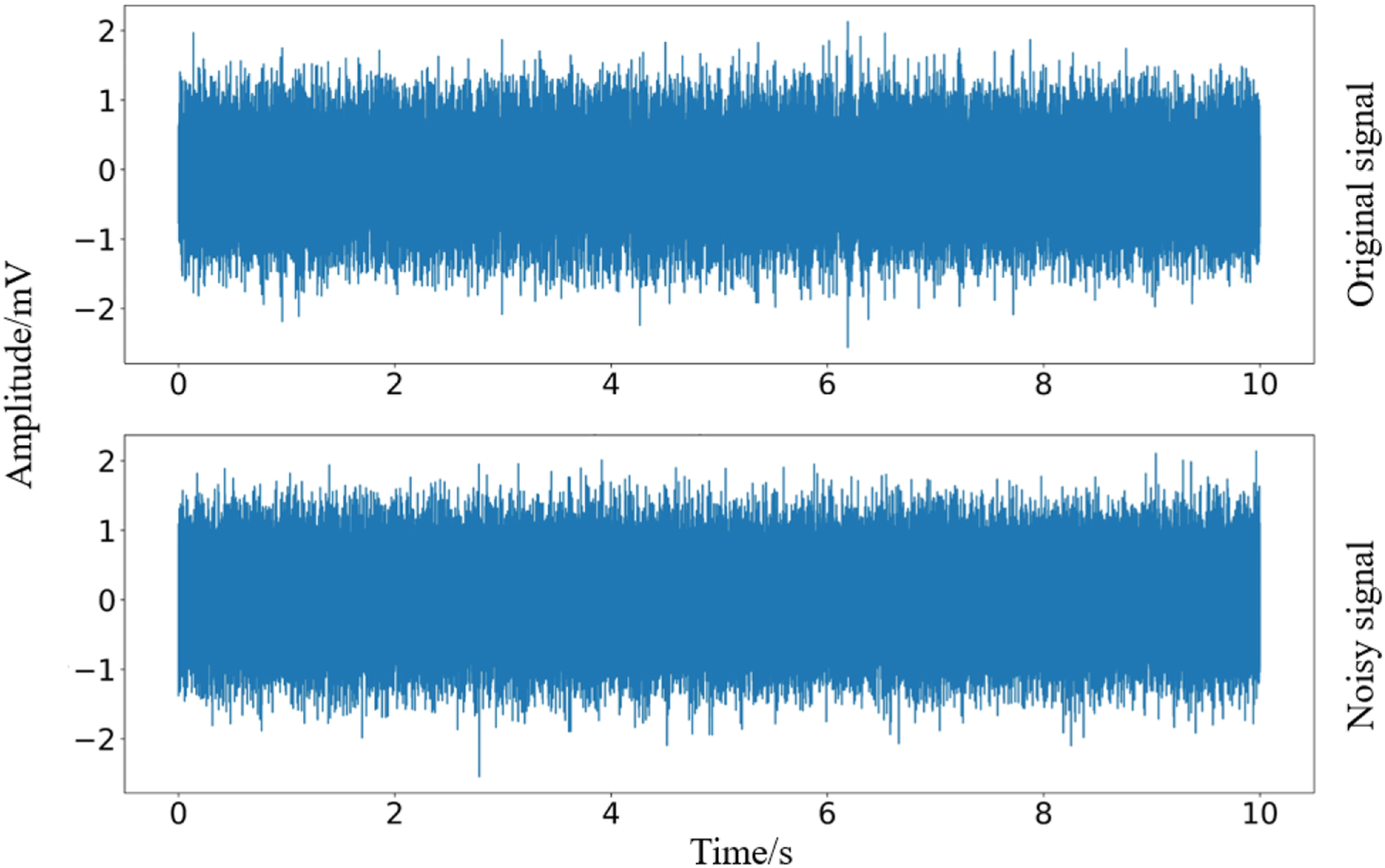

The signal added noise has an obvious feature coverage on the original signal, which has great interference on the subsequent fault diagnosis.

Taking the B014 fault signal in the 0 HP condition as an example, the above noisy signal is denoised by EMD ²¹ and SSA, and the denoising effects are compared.

First, EMD is used to decompose the noise signal to obtain a series of IMF components. The final noise reduction signal is obtained by superposing the corresponding components according to the variance contribution rate of each component. In this experiment, the first two IMF components are extracted from nine IMF components for superposition. The SNR of the noise reduction signal is reduced to −7.7018366 db through comparison with the original vibration signal. The time domain diagram of the signal after noise reduction is shown in Figure 4. Obviously, the noise reduction effect of EMD for large noise is not very ideal.

Figure 4.

Time domain diagram of empirical mode decomposition noise reduction signal.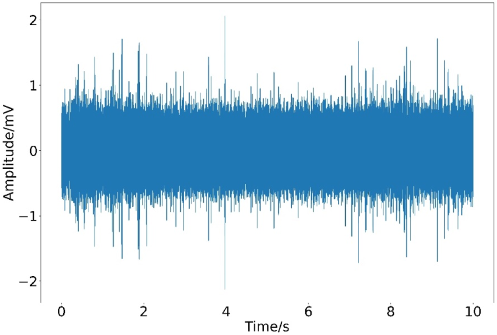

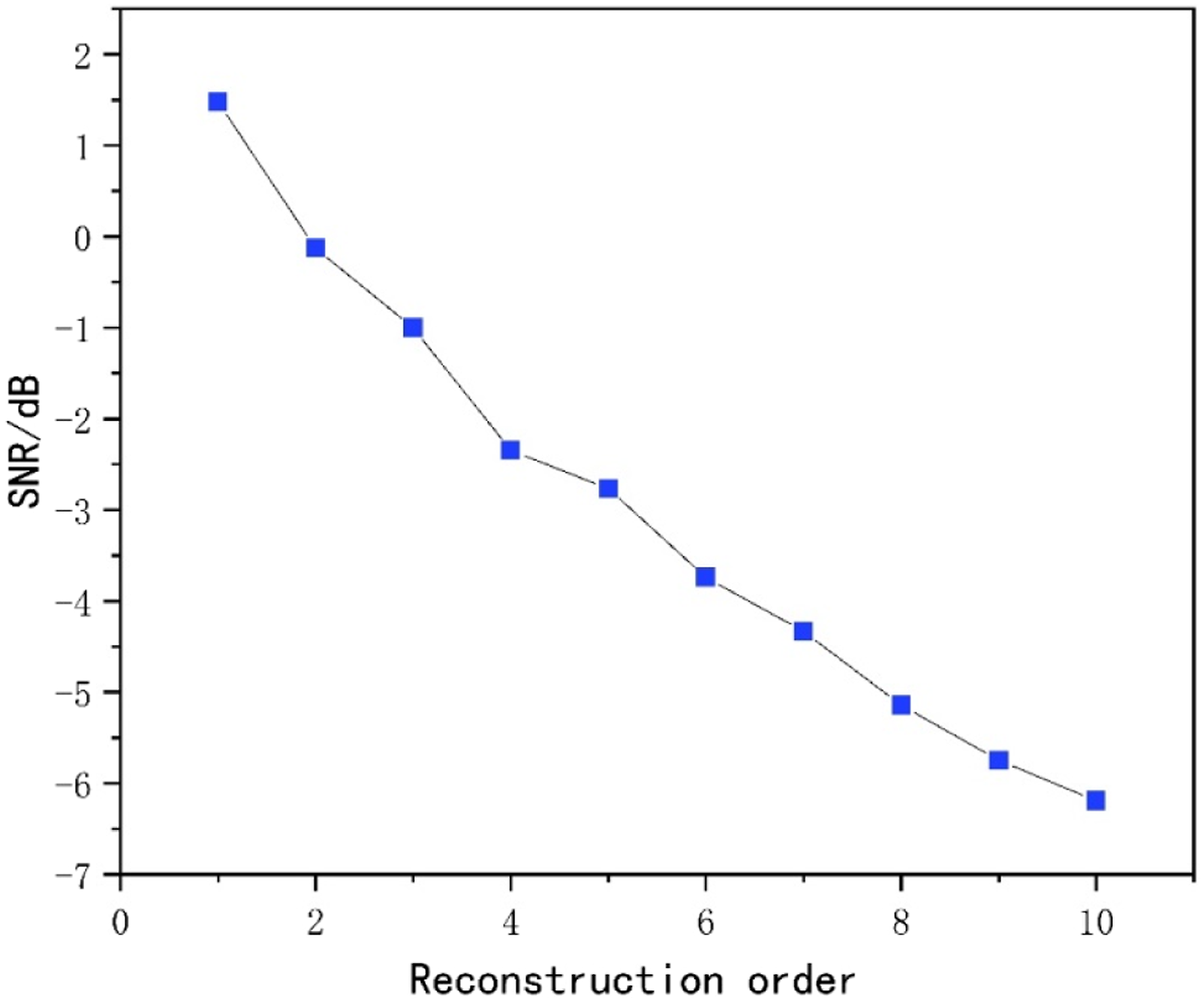
Then, SSA is used to denoise the same noisy signal. This test signal extracts the SVD components of orders 1–10, and each component is shown in Figure 5. In these 10 components, the appropriate components of the first several orders are selected for signal reconstruction, and the noise reduction effect of the specific order is shown in Figure 6. The noise reduction effect of the first-order signal component is the best, and the SNR of the denoised signal is 1.4750415449348 dB, which greatly eliminates the noise interference on the fault features and has a certain amplification gain effect on the original signal, which is conducive to the subsequent feature extraction work. The signal diagram after decomposition and reconstruction is shown in Figure 7. Compared with the original signal, it can be found that the peak characteristics of the reconstructed signal are more obvious, because the effective components are further retained after SSA noise reduction, while the redundant components will be more eliminated, the fault characteristics will be amplified accordingly, and the corresponding time domain diagram will show the characteristics of prominent peak.

Figure 5.

First 10 order singular value decomposition component signal graph.

Figure 6.

Noise reduction effect picture of multi order signal reconstruction.

Figure 7.

Time domain diagram of singular spectrum analysis noise reduction signal.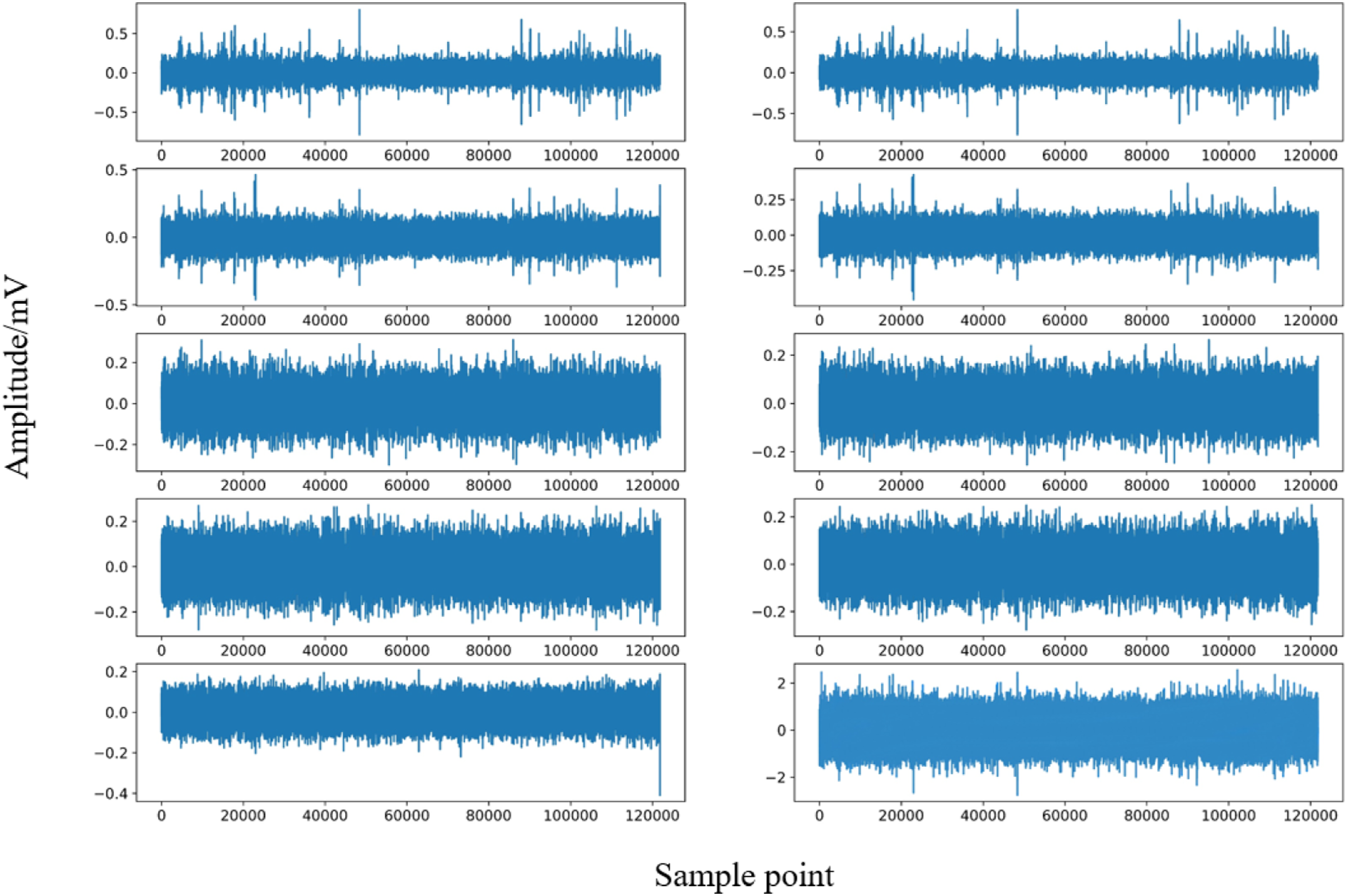

Validation of model diagnosis based on SSA-WDCNN

In this section, the fault diagnosis effects of four deep learning methods, namely, denoising AE CNNs (DAE-CNN), SSA-WDCNN, EMD-WDCNN, and AdmBN neural network, are compared for noise signals under the same working conditions to verify the practical value of the method. The fault signal with a SNR = −10 dB at 0 HP (1797 rpm) was selected to train and test the network model.

The structure parameters of the DAE-CNN constructed in this experiment are as follows: the convolution core width of the first convolution layer is 20, the number of convolution cores is 32, and the step size is 8; the pooling width of the first pooling layer is 4, the number of convolution cores is 32, and the step size is 4. Except for the first layer, the structure parameters of the layers are the same as those of the WDCNN in the Structural Parameters of WDCNN Model section, and BN is not performed in the middle of the neural network. The EMD-WDCNN mainly uses EMD noise reduction combined with the WDCNN architecture with the same parameters for fault diagnosis comparative test. The AdmBN neural network takes the traditional CNN as the main body and adds Adam gradient optimization and BN middle layer normalization to carry out the same condition fault diagnosis test. The batch size was set to 128 to train the two models 20 times.

The specific training effects of the four models are shown in Figures 8 and 9, including the curve changes of accuracy and loss during training.

Figure 8.

Change chart of model training accuracy.

Figure 9.

Model training loss chart.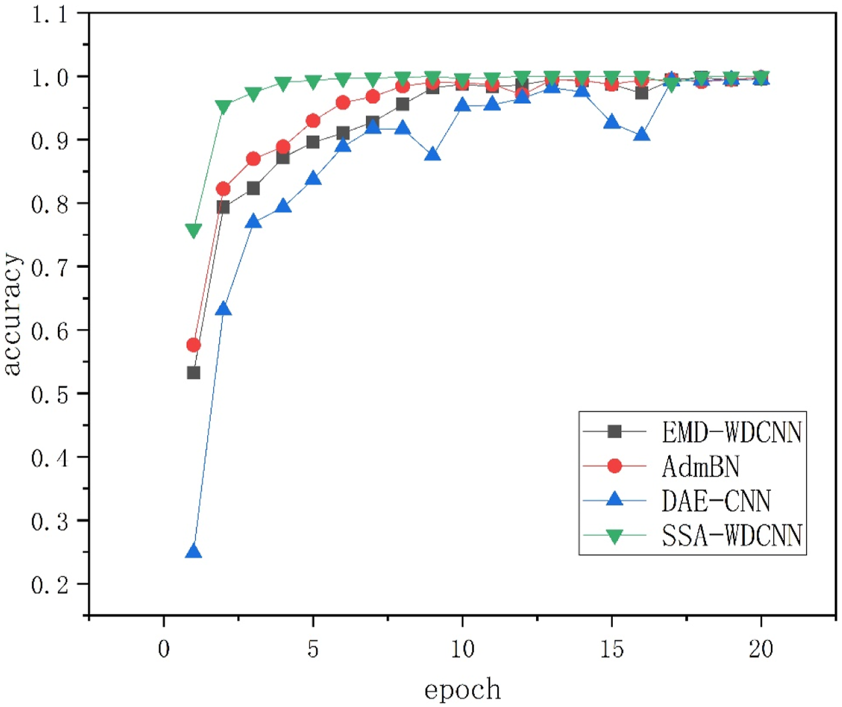

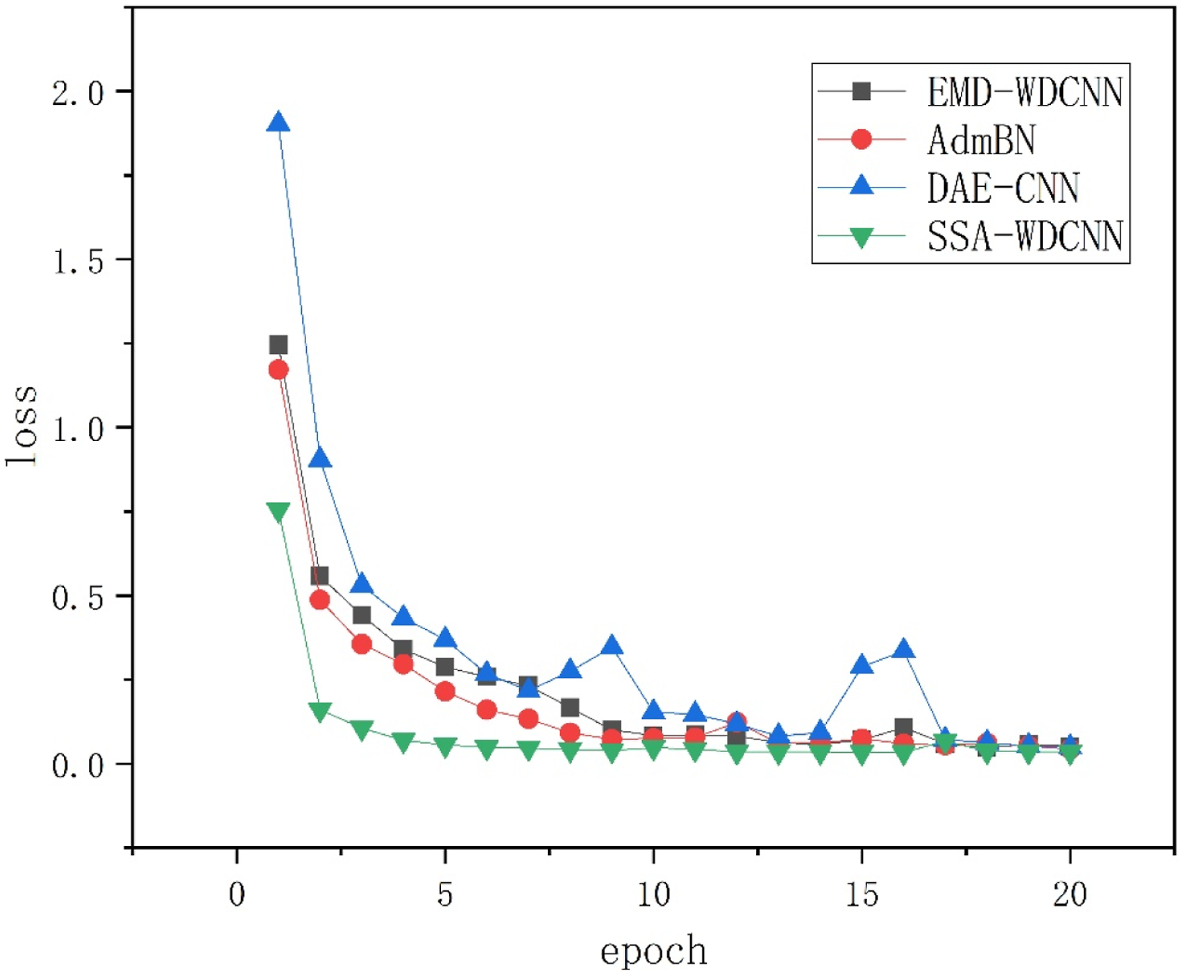
The analysis of the accuracy and loss of the four models indicate that the diagnosis model based on the SSA-WDCNN has a fast convergence, and the training effect of the model is relatively good and stable. Then, on the basis of the trained models, T-SNE dimensionality reduction visualization processing is performed for the final convolution layer feature extraction of the two methods. The distribution of features is shown in Figure 10.

Figure 10.

T-SNE visualization of feature extraction from four models: (a) denoising auto encoders-convolutional neural network, (b) singular spectrum analysis-WDCNN, (c) empirical mode decomposition-WDCNN, (d)AdmBN. WDCNN: wide convolution depth neural network.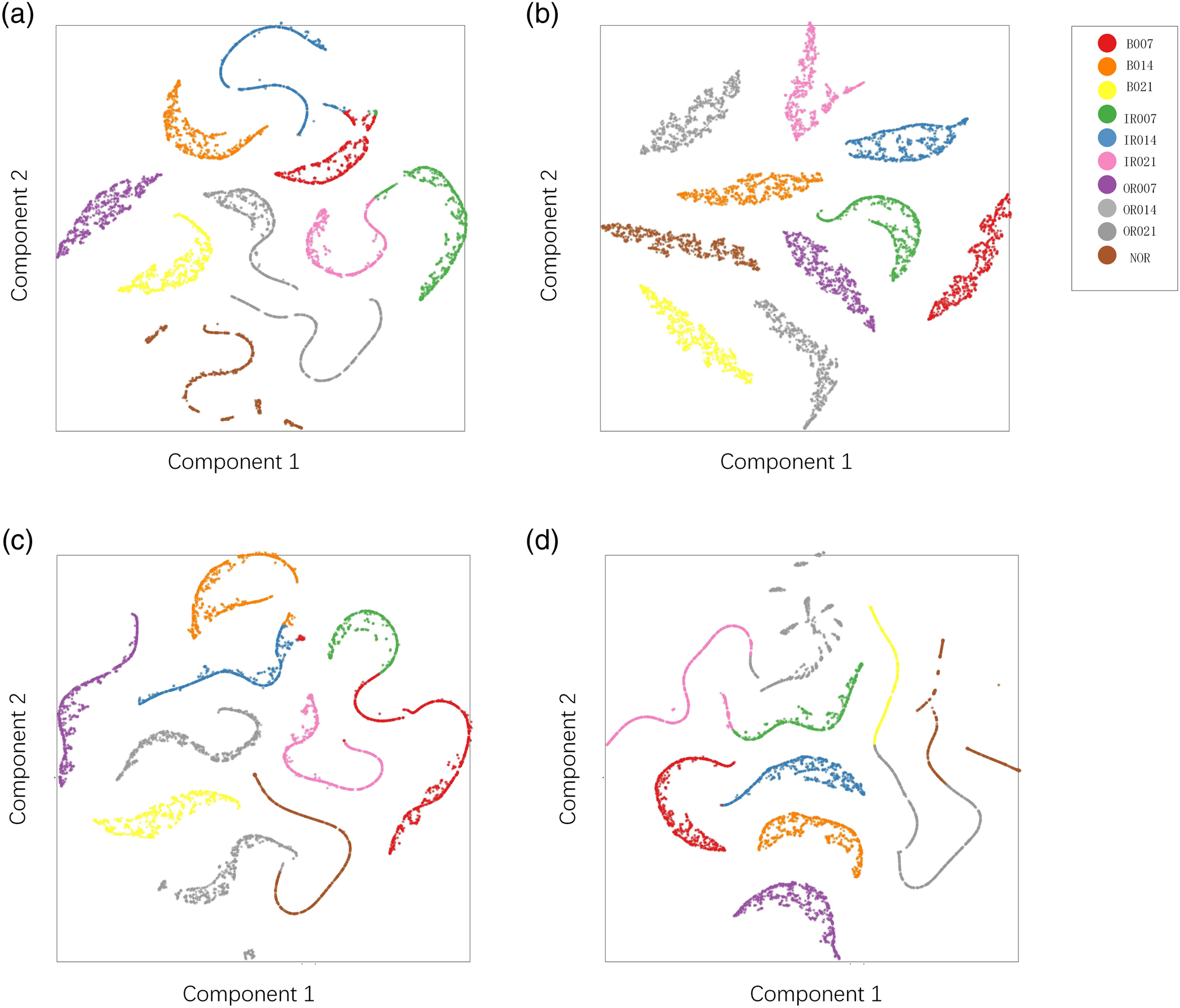

The visual comparison of the feature extraction of the last layer of the convolution layer of the four schemes indicates that the overall classification effect is still relatively ideal. The proposed SSA-WDCNN model has a good feature extraction ability. Meanwhile, confusion matrix analysis is performed on the test results of the four subsequent test sets, as shown in Figure 11. A series of comparisons shows that the proposed diagnosis model is effective.

Figure 11.

Confusion matrix of four models transferring results: (a) denoising auto encoders-convolutional neural network, (b) singular spectrum analysis-WDCNN, (c) empirical mode decomposition-WDCNN, (d)AdmBN. WDCNN: wide convolution depth neural network.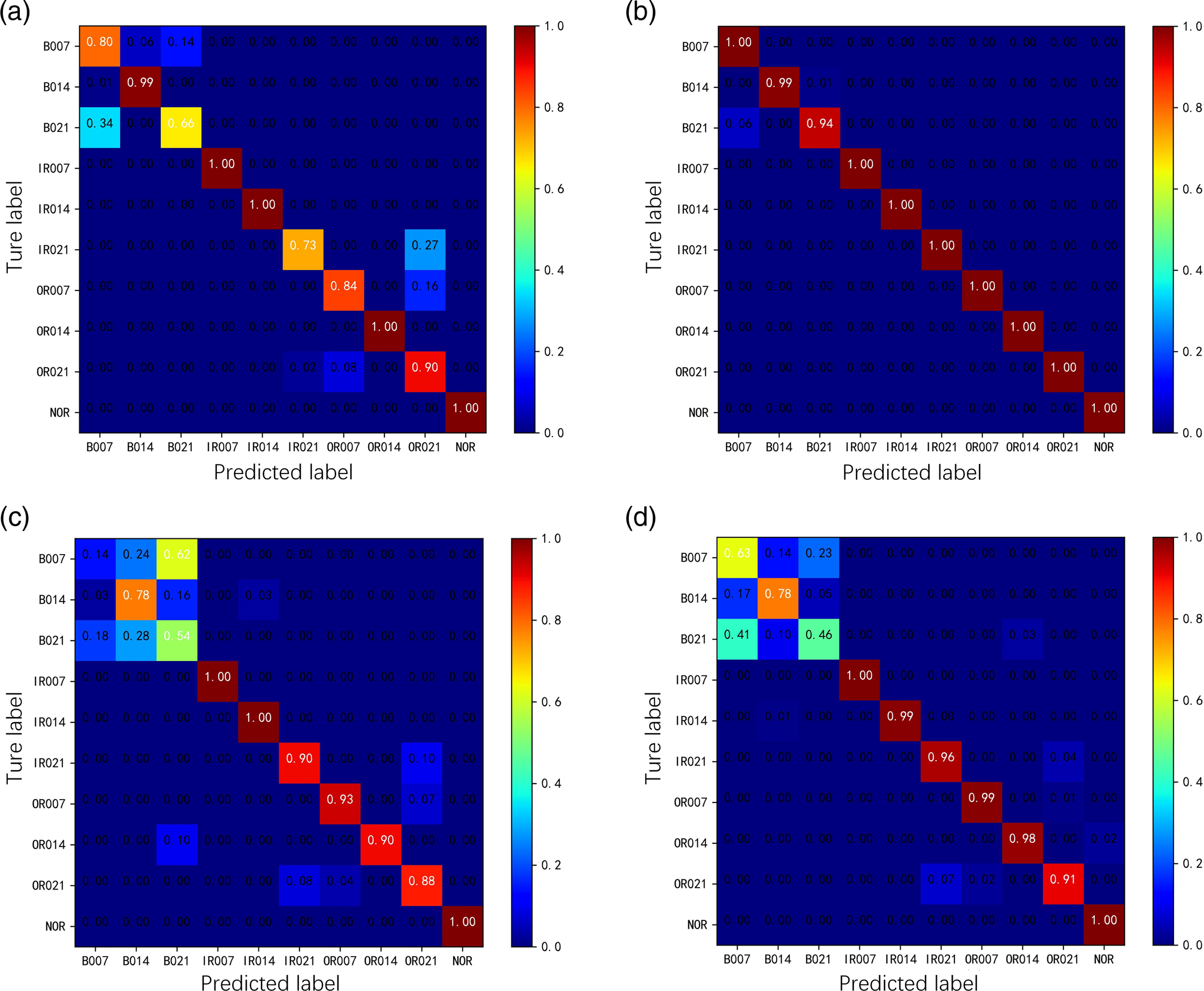

Through the completion of the above fault diagnosis contrast test, the excellent diagnosis performance of the proposed SSA-WDCNN in the case of large noise interference is proven. Among the four methods, the classification results of DAE-CNN do not have abrupt large error because of its good matching of double-layer noise reduction, but its stability is slightly insufficient. The diagnostic stability of AdmBN is very high after batch processing training, but the diagnostic error will be significantly great due to the lack of double-layer filter structure. Compared with the two methods, the diagnosis model combined with WDCNN network structure has better fault diagnosis effect. The batch processing speeds up the classification convergence rate and avoids the continuous classification confusion. Especially, when the two diagnosis models adopt the same deep neural network structure, the diagnosis accuracy of SSA-WDCNN is significantly better than EMD-WDCNN, which proves that SSA has better noise reduction effect on the fault signal of rolling bearing. At the same time, the overall error of SSA-WDCNN model remains stable in terms of model diagnosis learning efficiency and stability, The EMD-WDCNN model needs to learn and classify for many times before the accuracy of fault diagnosis tends to be stable. Under the comprehensive comparison, SSA and WDCNN network structure have a better fit, and the model is also more excellent in the fault diagnosis of rolling bearings. The above four methods are selected from the range of −10 dB–0 dB for the environmental interference diagnosis contrast test. The test condition remains at 0 hp (1797 rpm). The results of the test are shown in Table 2.

Table 2.

Fault diagnosis effect of four models in multi noise environment.

Signal-to-noise ratio/dB	Diagnostic accuracy of four models/%
	Empirical mode decomposition-WDCNN	AdBN	Denoising auto encoder-convolutional neural network	Singular spectrum analysis-WDCNN
0	99.7	99.3	99.1	99.9
−2	97.4	97.3	98.6	99.3
−4	94.3	97.3	97.4	99.0
−6	89.1	92.9	94.7	98.7
−8	81.4	87.0	92.4	93.9
−10	80.7	82.1	65.4	93.7

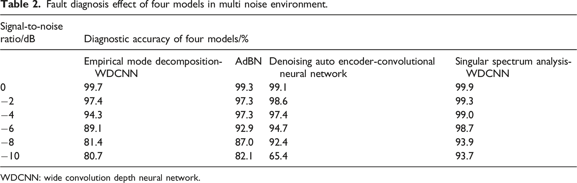
WDCNN: wide convolution depth neural network.

Through the above comparative test analysis, the advantages of the model are shown in the following aspects: the training loss chart of the model and the feature classification visualization of the neural network reflect that the feature extraction and integration function of WDCNN is hierarchical and effective. On this basis, the error matrix compares and highlights the positive anti-interference of the first layer SSA noise reduction purification. With the combination of the two, the diagnostic data of the diagnostic model is extremely efficient and stable.

Anti-interference verification of multi-working conditions

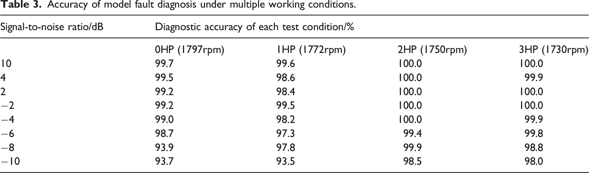
In the previous section, the bearing fault diagnosis model based on the SSA-WDCNN is proven to have better training effect and test accuracy than the DAE-CNN model. In this section, the model is tested under multiple working conditions, and the fault diagnosis test is carried out for the vibration signal with eight kinds of noise: −10, −8, −6, −4, −2, 2, 4, and 10 dB. The anti-interference and generalization abilities of the model are determined by analyzing the overall diagnosis effect.

Table 3 shows that the specific diagnosis effect of the bearing fault diagnosis model based on the proposed WDCNN is relatively stable in multiple working conditions, and the overall diagnosis effect remains above 93%. For the same SNR interference vibration signal, the model has the best diagnosis effect at 2 HP (1750 rpm), and the accuracy exceeds 99%, while the accuracy is relatively small at 1 hp (1772 rpm) but can also exceed 93.5%. Therefore, the influence of different working conditions on the diagnosis accuracy of the model is controllable. The overall SNR of the model remains high in the face of interference. The results show that the proposed method of decomposition and reconstruction of noisy signal by SSA combined with feature extraction and the classification of denoising signal by the WDCNN completes the fault diagnosis, which has a high accuracy and a stable diagnosis effect in the face of multi-working conditions and high noise.

Table 3.

Accuracy of model fault diagnosis under multiple working conditions.

Signal-to-noise ratio/dB	Diagnostic accuracy of each test condition/%
	0HP (1797rpm)	1HP (1772rpm)	2HP (1750rpm)	3HP (1730rpm)
10	99.7	99.6	100.0	100.0
4	99.5	98.6	100.0	99.9
2	99.2	98.4	100.0	100.0
−2	99.2	99.5	100.0	100.0
−4	99.0	98.2	100.0	99.9
−6	98.7	97.3	99.4	99.8
−8	93.9	97.8	99.9	98.8
−10	93.7	93.5	98.5	98.0

Conclusion

(1) An improved convolution neural network model is used in fault signal feature extraction. The advantage is that the model uses a large convolution kernel for the first layer convolution processing to complete short-term feature extraction and then uses a small convolution kernel to increase the network depth to achieve sensitive feature extraction and classification. The average iteration time is 24 ms, and the overall efficiency is greatly improved by adding a BN layer to ensure convergence stability during training. The improvement of this structure can avoid the excessive extraction of fault features after signal passing through SSA, and improve the fit of double-layer filter structure.

(2) The rolling bearing diagnosis method based on singular value analysis and wide convolution kernel neural network proposed in this paper aims to strengthen the extraction of fault features and improve the diagnosis accuracy by multi-layer filtering. By analyzing the diagnosis results of multiple groups of noise in the range of −10 dB–0 dB, it is found that the diagnosis stability of the model will be greatly reduced after −6 dB. The feature extraction matching between SSA-WDCNN model proposed in this paper is more efficient than other methods, so the overall accuracy can be maintained at more than 93%. In the multi condition test, it can also be clearly found that the diagnostic accuracy will decline in a certain noise range. Although the diagnostic accuracy remains at a high level, it has a downward trend. Therefore, the follow-up research will further improve the network structure, optimize the matching degree of singular spectrum decomposition parameters, and strengthen the diagnostic stability and accuracy of the model under changeable or abrupt noise.