Sage Journals: Discover world-class research

Abstract

Nonlinear vibration arises everywhere in a bistable system. The bistable system has been widely applied in physics, biology, and chemistry. In this article, in order to numerically simulate a class of space fractional-order bistable system, we introduce a numerical approach based on the modified Fourier spectral method and fourth-order Runge-Kutta method. The fourth-order Runge-Kutta method is used in time, and the Fourier spectrum is used in space to approximate the solution of the space fractional-order bistable system. Numerical experiments are given to illustrate the effectiveness of this method.

Keywords

Space fractional bistable system Fourier spectral method fractional Laplacian numerical simulation

Introduction

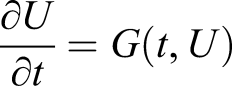
Fractional partial differential equations are becoming widely used as a suitable modeling approach for many fields in science and engineering.^1–6 We mainly study models arising in the application areas of theoretical biology, physics, and chemistry, modeled by some space fractional bistable systems

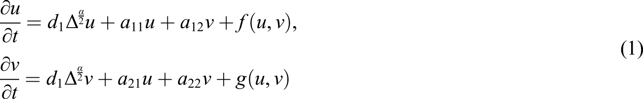
\begin{array}{l} \frac{\partial u}{\partial t} = d_{1} Δ^{\frac{α}{2}} u + a_{11} u + a_{12} v + f (u, v), \\ \frac{\partial v}{\partial t} = d_{1} Δ^{\frac{α}{2}} v + a_{21} u + a_{22} v + g (u, v) \end{array}

(1)

where u = u (x, y, t) and v = v (x, y, t) are unknown functions. $(x, y) \in Ω = [a, b] \times [c, d], t > 0$ , the smooth boundary is $\partial Ω$ . The parameters d_i, i = 1 and 2 ∈ R⁺ are diffusion coefficients, and f (u_i, v_i) and g (u_i, v_i) are the reaction terms. The system (1) is subjected to some initial condition u (x, y, 0) = u₀ (x, y), v (x, y, 0) = v₀ (x, y), and the homogeneous Neumann boundary condition, namely, $\frac{\partial u}{\partial n} \cdot \partial Ω = \frac{\partial v}{\partial n} \partial Ω = 0$ . The functions u (x, y, t) and v (x, y, t) are assumed to be a causal function of time, that is, vanishing for t < 0. The general response expression contains parameters describing the order of the fractional derivatives that can be varied to obtain various responses. In this article, we use the fractional Laplacian operator by the Riesz fractional derivatives as follows

Δ^{\frac{α}{2}} u = \frac{\partial^{α} u}{\partial {| x |}^{α}} + \frac{\partial^{α} u}{\partial {| y |}^{α}} = \frac{1}{2 \cos \frac{π α}{2}} {}_{x}D_{R}^{α} u + {}_{x}D_{R}^{α} u + {}_{y}D_{L}^{α} u + {}_{y}D_{R}^{α} u

(2)

with

{}_{x}D_{L}^{α}, {}_{x}D_{R}^{α} u and {}_{y}D_{L}^{α} u, {}_{y}D_{R}^{α} u

being the RiemannLiouville fractional operators.

Many approaches are used to solve the reaction-diffusion system. These methods include the finite difference method,⁷ reproducing the kernel method (RKM),^8–17 variational iteration method (VIM),^18–19 homotopy perturbation methods (HPM),^20–22 etc.^23–27 There are few numerical methods for higher order space fractional reaction-diffusion system.

In this article, in order to numerically simulate space fractional-order reaction-diffusion system, we introduce a novel numerical approach based on the modified Fourier spectral method^28–30 and fourth-order Runge-Kutta method. Some pattern formations are shown by using this new approach, and the results have good agreement with theoretical results. Simulation results show the effectiveness of the method.

Bifurcation analysis of system

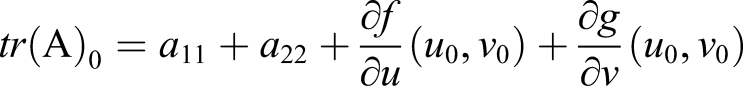
In this section, we give the Turing bifurcation conditions of system (1). We assume the equilibrium point of the non-diffusive system (1) is E^∗ = (u₀, v₀), so

\begin{array}{l} a_{11} u_{0} + a_{12} v_{0} + f (u_{0}, v_{0}) = 0, \\ a_{11} u_{0} + a_{12} v_{0} + g (u_{0}, v_{0}) = 0 \end{array}

(3)

Now, we do linear stability analysis of the equilibrium point E^∗. We evaluate the Jacobian matrix A₀ of the system at E^∗ as

g (t - \hat{u}) =

(4)

The characteristic roots for $A_{0}$ are given by

λ_{1,2} (0) = \frac{1}{2} [t r {(A)}_{0} \pm \sqrt{{[t r {(A)}_{0}]}^{2} - 4 \det {(A)}_{0}}]

(5)

where

t r {(A)}_{0} = a_{11} + a_{22} + \frac{\partial f}{\partial u} (u_{0}, v_{0}) + \frac{\partial g}{\partial v} (u_{0}, v_{0})

and

\det {(A)}_{0} = [a_{11} + \frac{\partial f}{\partial u} (u_{0}, v_{0})] \times [a_{22} + \frac{\partial g}{\partial v} (u_{0}, v_{0})] - [a_{21} + \frac{\partial g}{\partial u} (u_{0}, v_{0})] \times [a_{12} + \frac{\partial f}{\partial v} (u_{0}, v_{0})]

In general, if real part of eigenvalues λ_1,2 (0) is negative, then the non-diffusive system (1) is stable.

Next, we derive cross-diffusion driven instability conditions and show that these are a generalization of the classical diffusion-driven instability conditions in the absence of cross-diffusion.

A_{α} = \begin{matrix} b_{11} \\ b_{21} \end{matrix} \begin{matrix} b_{12} \\ b_{22} \end{matrix} - \begin{matrix} d_{11} \\ d_{21} \end{matrix} \begin{matrix} d_{12} \\ d_{22} \end{matrix}

(6)

where

b_{11} = a 11 + \frac{\partial f}{\partial u} (u_{0}, v_{0}), b_{12} = a_{12} + \frac{\partial f}{\partial v} (u_{0}, v_{0}), b_{21} = a_{21} + \frac{\partial g}{\partial u} (u_{0}, v_{0}), b_{22} = a_{22} + \frac{\partial g}{\partial v} (u_{0}, v_{0})

The characteristic roots for $A_{α}$ are given by

λ_{1,2} (α) = \frac{1}{2} [t r (A_{α}) \pm \sqrt{{[t r (A_{α})]}^{2} - 4 \det (A_{α})}]

(7)

where

t r (A_{α}) = b_{11} + b_{22} - α (d_{11} + d_{22})

and

\det (A_{α}) = (d_{11} d_{22} - d_{12} + d_{21}) α^{2} - (b_{11} d_{22} + b_{22} d_{11} - b_{12} d_{21}) α + (b_{11} d_{22} - b_{12} d_{21})

Turing bifurcation occurs when the equilibrium state is stable in absence of non-diffusion but it becomes unstable in presence of cross-diffusion. Thus, the only way for the E^∗ to become an unstable point of the cross-diffusion system (1) is when the real part of eigenvalues λ_1,2 (k) is positive; then, the cross-diffusion system (1) is unstable.

Fourier spectral method

For any integer N > 0, consider $x_{j} = j Δ x = \frac{2 π L j}{N}, y_{j} = j Δ y = \frac{2 π L j}{N}, L = b - a, j = 0,1, \dots, N - 1$ . $u (x, y, t)$ is transformed into the discrete Fourier space as

\hat{u} (k_{x}, k_{y}, t) = F (u) = \frac{1}{N^{2}} \sum_{j = 0}^{N - 1} \sum_{j = 0}^{N - 1} u (x_{j}, y_{j}, t) e^{- i k_{x} x j - i k_{y} y j} - \frac{N}{2} \leq k_{x}, k_{y} \leq \frac{N}{2} - 1

(8)

and the inverse formula is

u (x_{j}, y_{j}, t) = F^{- 1} (\hat{u}) = \sum_{k_{x} = - \frac{N}{2}}^{N - 2} \sum_{k y = - \frac{N}{2}}^{N - 2} \hat{u} (k_{x}, k_{y}, t) e^{- i k_{x} x j - i k_{y} y j}, 0 \leq j \leq N - 1

(9)

It is easy to know u (x, y, t) = $F^{- 1} {F [u (x, y, t)]}$ .

For system (1) with $f (u, v) = r (a - u + u^{2} v)$ and $g (u, v) = r (b - u^{2} v)$ , using Fourier transform, we can get

\begin{array}{l} \frac{\partial \hat{u}}{\partial t} = d_{1} {(i k_{x})}^{α} + {(i k_{y})}^{α} \hat{u} + a_{12} F {F^{- 1} [\hat{u}]} + a_{12} F {F^{- 1} [\hat{v}]} + r (a - F {F^{- 1} [\hat{u}] + F^{- 1} {[\hat{u}]}^{2} F^{- 1} [\hat{v}]}) \\ \frac{\partial \hat{v}}{\partial t} = d_{2} {(i k_{x})}^{α} + {(i k_{y})}^{α} \hat{u} + a_{22} F {F^{- 1} [\hat{u}]} + a_{22} F {F^{- 1} [\hat{v}]} + r (b - F {F^{- 1} {[\hat{u}]}^{2} F^{- 1} [\hat{v}]}) \end{array}

(10)

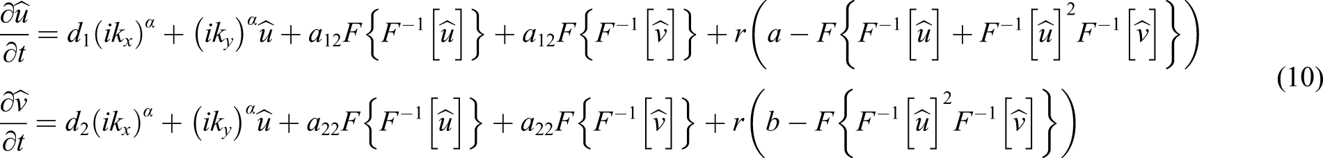
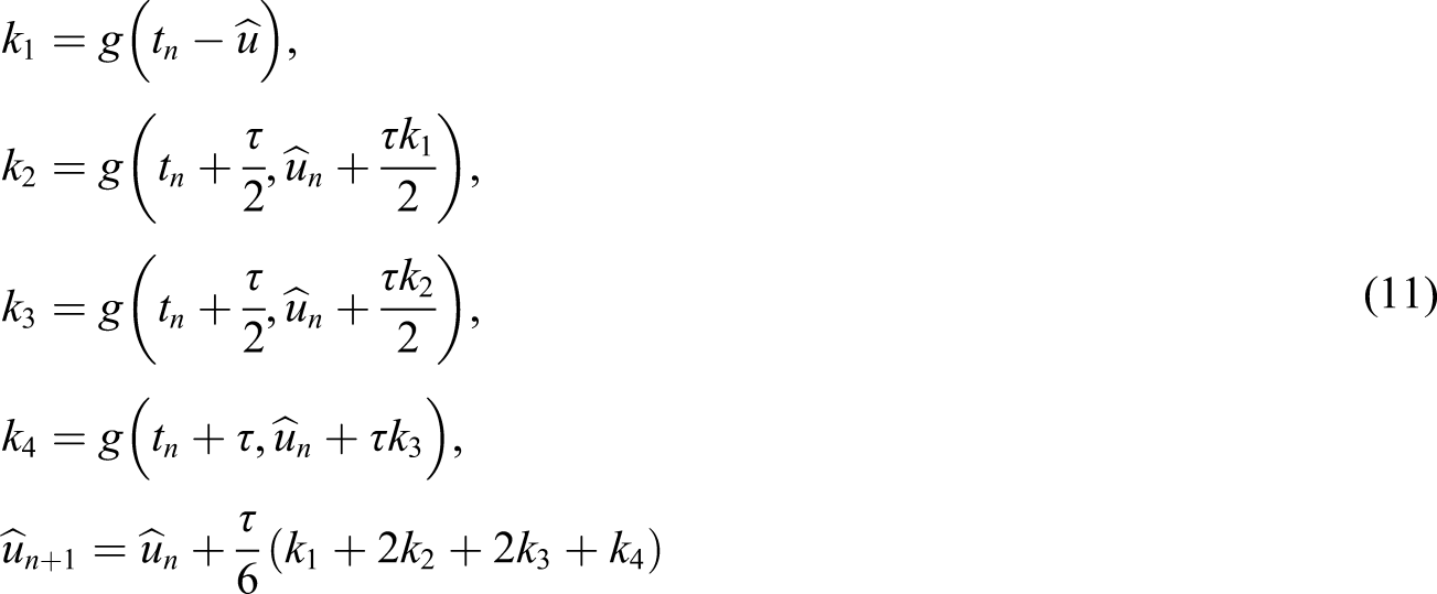
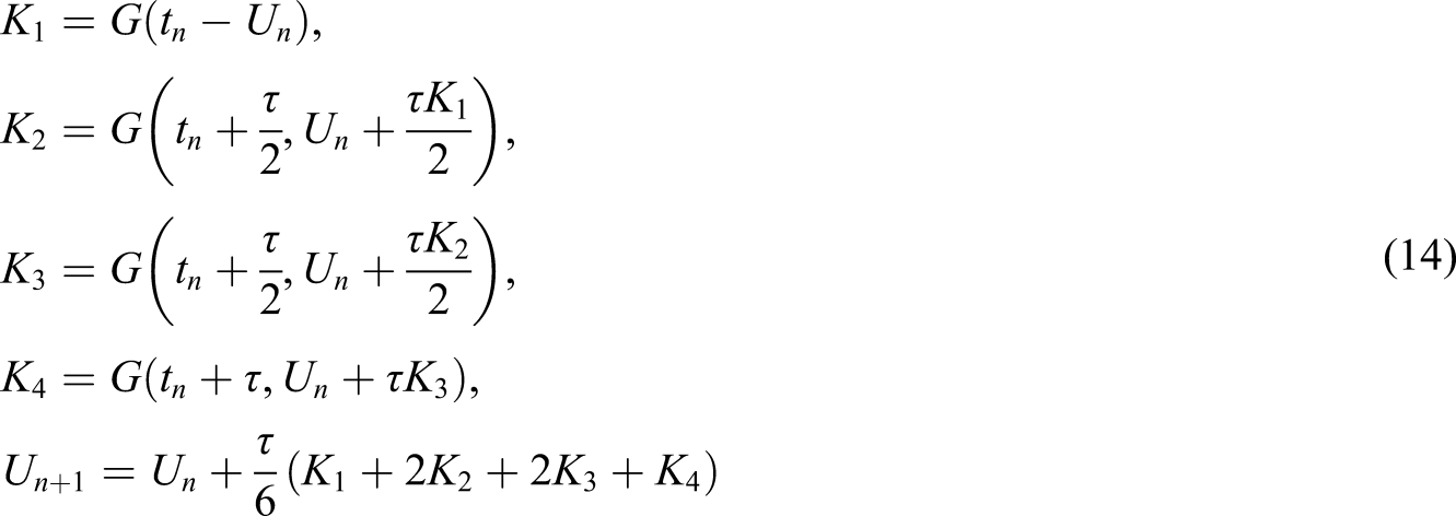
We use the fourth-order Runge-Kutta method to solve the ordinary differential equation (10) which is as follows

\begin{array}{l} k_{1} = g (t_{n} - \hat{u}), \\ k_{2} = g (t_{n} + \frac{τ}{2}, {\hat{u}}_{n} + \frac{τ k_{1}}{2}), \\ k_{3} = g (t_{n} + \frac{τ}{2}, {\hat{u}}_{n} + \frac{τ k_{2}}{2}), \\ k_{4} = g (t_{n} + τ, {\hat{u}}_{n} + τ k_{3}), \\ {\hat{u}}_{n + 1} = {\hat{u}}_{n} + \frac{τ}{6} (k_{1} + 2 k_{2} + 2 k_{3} + k_{4}) \end{array}

(11)

where

τ

is step-size and

g (t - \hat{u}) = \frac{\partial \hat{u}}{\partial t} / \frac{\partial \hat{v}}{\partial t}

. For convenience of expression, we denote

U = {({\hat{u}}_{0} (t), {\hat{u}}_{1}, \dots, {\hat{u}}_{N - 1} (t))}^{T}, G (t, U) = (g (t, \hat{u} (t)), g (t, \hat{u} (t))), n = 1, \dots \frac{T}{τ}

(12)

Equation (10) is reduced to

\frac{\partial U}{\partial t} = G (t, U)

Next, we can obtain the standard fourth-order Runge-Kutta formula

\begin{array}{l} K_{1} = G (t_{n} - U_{n}), \\ K_{2} = G (t_{n} + \frac{τ}{2}, U_{n} + \frac{τ K_{1}}{2}), \\ K_{3} = G (t_{n} + \frac{τ}{2}, U_{n} + \frac{τ K_{2}}{2}), \\ K_{4} = G (t_{n} + τ, U_{n} + τ K_{3}), \\ U_{n + 1} = U_{n} + \frac{τ}{6} (K_{1} + 2 K_{2} + 2 K_{3} + K_{4}) \end{array}

(14)

Then, we can derive that by solving the following formula

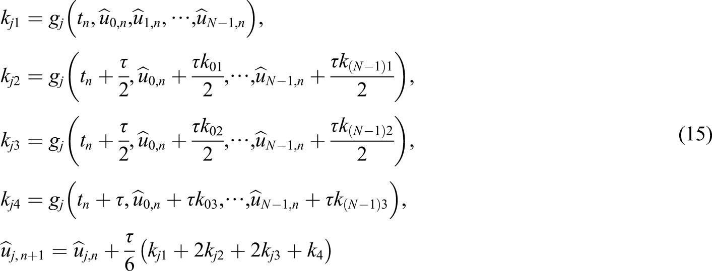
\begin{array}{l} k_{j 1} = g_{j} (t_{n}, {\hat{u}}_{0, n}, {\hat{u}}_{1, n}, \dots, {\hat{u}}_{N - 1, n}), \\ k_{j 2} = g_{j} (t_{n} + \frac{τ}{2}, {\hat{u}}_{0, n} + \frac{τ k_{01}}{2}, \dots, {\hat{u}}_{N - 1, n} + \frac{τ k_{(N - 1) 1}}{2}), \\ k_{j 3} = g_{j} (t_{n} + \frac{τ}{2}, {\hat{u}}_{0, n} + \frac{τ k_{02}}{2}, \dots, {\hat{u}}_{N - 1, n} + \frac{τ k_{(N - 1) 2}}{2}), \\ k_{j 4} = g_{j} (t_{n} + τ, {\hat{u}}_{0, n} + τ k_{03}, \dots, {\hat{u}}_{N - 1, n} + τ k_{(N - 1) 3}), \\ {\hat{u}}_{j, n + 1} = {\hat{u}}_{j, n} + \frac{τ}{6} (k_{j 1} + 2 k_{j 2} + 2 k_{j 3} + k_{4}) \end{array}

(15)

Finally, we find the numerical solution using the inverse discrete Fourier transform.²⁸

Numerical simulation

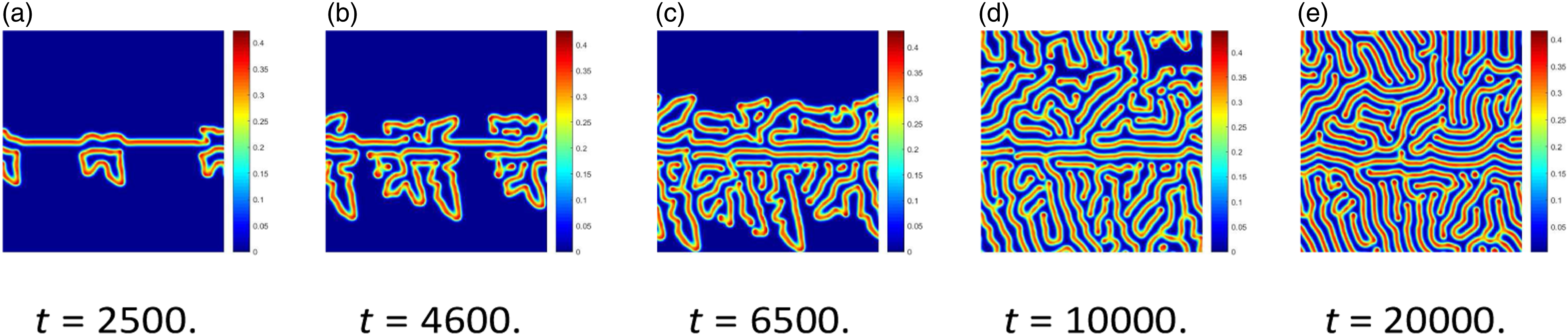
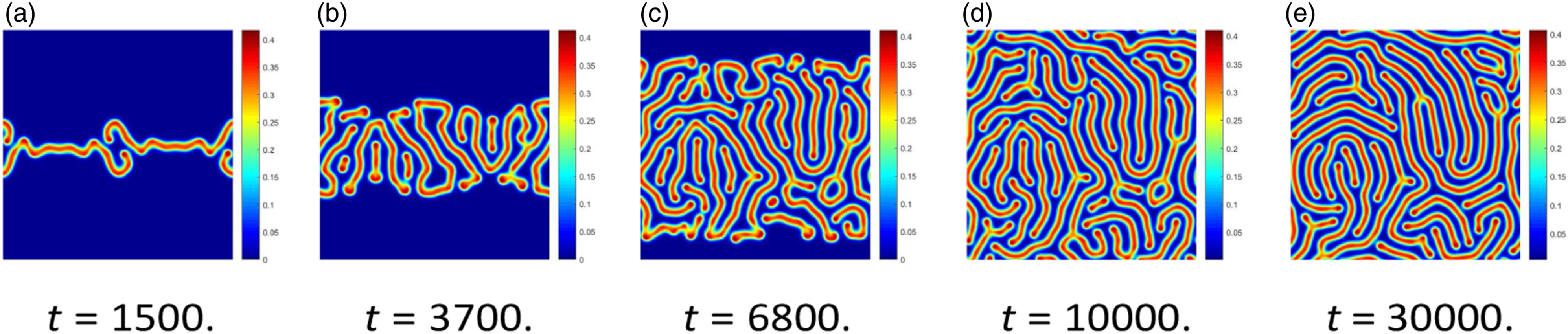
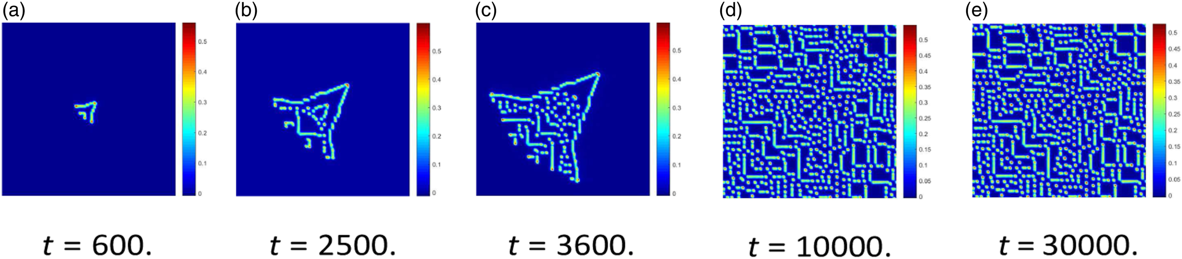
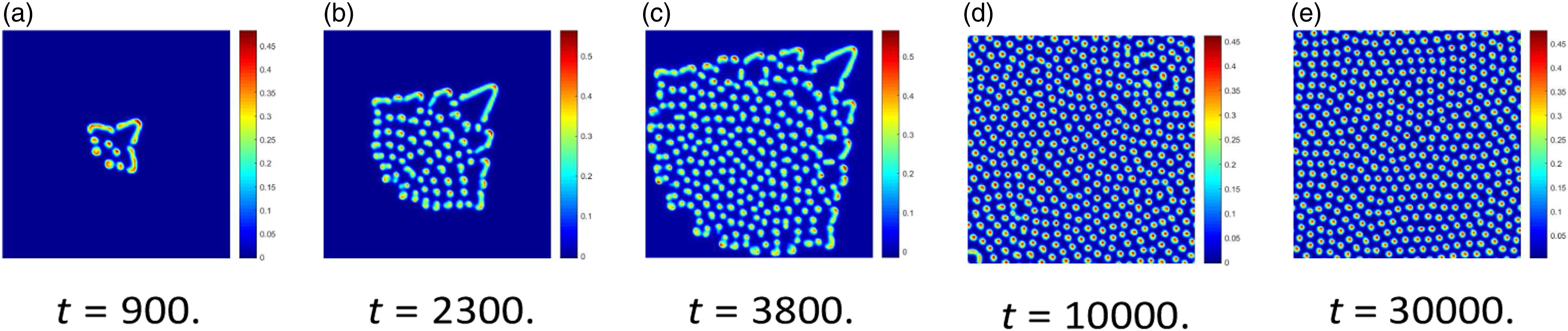
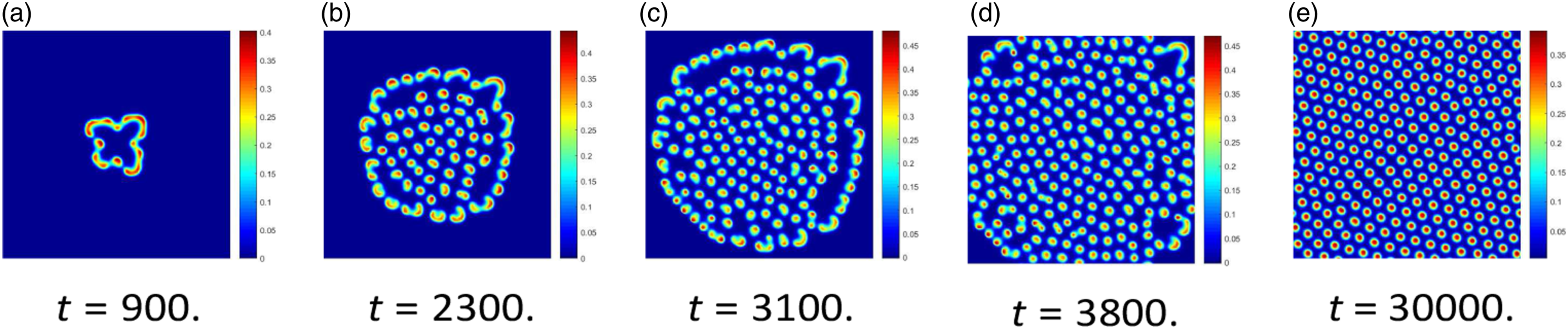
In this section, numerical simulation of the fractional Gray-Scott (GS) model with a perturbation to the spatially homogeneous steady-state equation is obtained. The domain of interest is taken to be Ω = [−1, 1]², discretized using N = 128 points in each spatial coordinate. On account of the evolution of the numerical solution, u is similar with that of the v, but we will not present it in this article.

Numerical experiment Consider the following fractional Gray-Scott (GS)³¹ model:

\begin{array}{l} \frac{\partial u}{\partial t} = d_{1} (Δ^{\frac{α}{2}}) u - u v^{2} + F (1 - u), \\ \frac{\partial v}{\partial t} = d_{2} (Δ^{\frac{α}{2}}) v - u v^{2} + (F + k) v, (x, y, t) \in Ω \times [0, T] \end{array}

(16)

We take d₁ = 2 × 10⁻⁵, d₂ = 1 × 10⁻⁵, F = 0.045, k = 0.0625, u = ones (N), v = zeros (N), $v (N / 2, N / 2 : N) = 0.5, v (N / 2 - 1, 1 : N / 2) = 1$ , the numerical results are shown in Figures 1 and 2. We take d₁ = 2 × 10⁻⁵, d₂ = 1 × 10⁻⁵, F = 0.045, k = 0.0625, u = ones (N), v = zeros (N), $v (N / 2, N / 2 : N) = 0.5, v (N / 2 - 2, 1 : N / 2) = 1$ , the numerical results are shown in Figure 3. We take d₁ = 3×10⁻⁵, d₂ = 1×10⁻⁵, F = 0.015, k = 0.055, u = ones (N), v = zeros (N), $v (N / 2, N / 2 : N) = 0.5, v (N / 2 - 2, 1 : N / 2) = 1$ ; the numerical results are shown in Figures 4–6.

Figure 1.

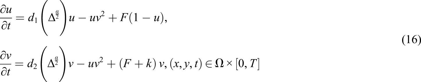
Numerical solutions at different α = 2, d₁ = 2 × 10⁻⁵, F = 0.045, k = 0.0625. (a) t = 2100. (b) t = 4400. (c) t = 6700. (d) t = 10,000. (e) t = 30,000.

Figure 2.

Numerical solutions at different α = 1.9, d₁ = 2 × 10⁻⁵, F = 0.045, k = 0.0625. (a) t = 2500. (b) t = 4600. (c) t = 6500. (d) t = 10,000. (e) t = 20,000.

Figure 3.

Numerical solutions at different α = 2, d₁ = 2 × 10⁻⁵, F = 0.045, k = 0.0625. (a) t = 600. (b) t = 2500. (c) t = 3600. (d) t = 10,000. (e) t = 30,000.

Figure 4.

Numerical solutions at different α = 1.7, d₁ = 3 × 10⁻⁵, F = 0.015, k = 0.055. (a) t = 900. (b) t = 2300. (c) t = 3800. (d) t = 10000. (e) t = 30000.

Figure 5.

Numerical solutions at different α = 1.8, d₁ = 3 × 10⁻⁵, F = 0.015, k = 0.055. (a) t = 900. (b) t = 2300. (c) t = 3800. (d) t = 10,000. (e) t = 30,000

Figure 6.

Numerical solutions at different α = 1.9, d₁ = 3 × 10⁻⁵, F = 0.015, k = 0.055. (a) t = 900. (b) t = 2300. (c) t = 3100. (d) t = 3800. (e) t = 30,000.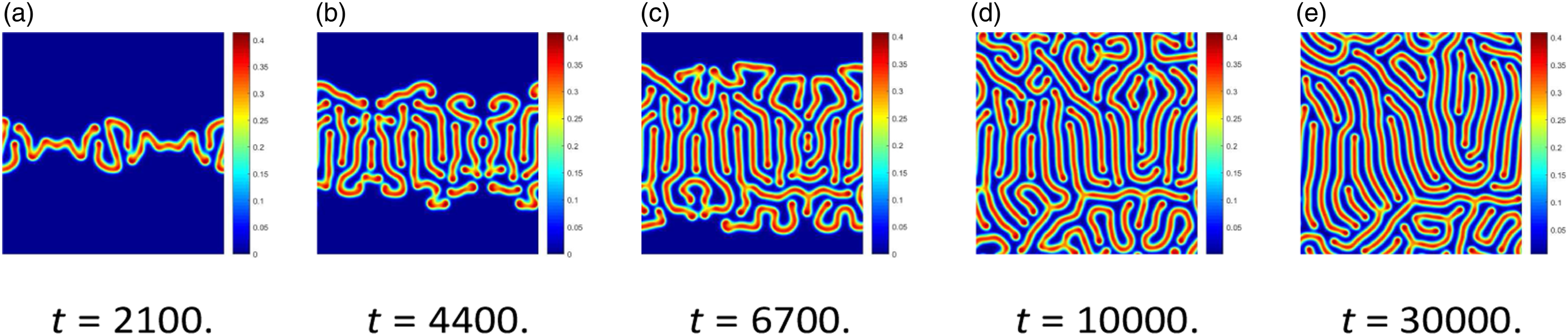

Conclusion and remarks

In the article, a numerical method that combines the Fourier spectral method with the Runge-Kutta method is proposed to study a class of space fractional bistable system. This approach has general meanings and thus can be used to solve same types of nonlinear space fractional partial differential equations with periodic boundary condition in science and engineering. Some pattern formations are shown by using this new approach, and the results have good agreement with theoretical results. Simulation results show the effectiveness of the method.

All computations are performed by the MATLABR2017b software.

Footnotes

Acknowledgments

The authors would like to express their thanks to the unknown referees for their careful reading and helpful comments.

Declaration of Conflicting Interests

The authors declared no potential conflicts of interest with respect to the research, authorship, and/or publication of this article.

Funding

The authors disclosed receipt of the following financial support for the research, authorship, and/or publication of this article: This work is supported by Inner Mongolia Natural Science Foundation under grant numbers (2021MS01009 and 2019MS07008).

ORCID iD

Wang Yulan

References

Jena

Chakraverty

Jena

, et al. Analysis of time-fractional fuzzy vibration equation of large membranes using double parametric based Residual power series method. ZAMM-J Appl Math Mech 2021; 101: e202000165.

Fikret

Aliev

Safarova

. Mamedova solution of the problem of analytical construction of optimal regulators for a fractional order oscillatory system in the general case. J Appl Comput Mech 2021; 7: 970–976.

El-Dib

. A tutorial introduction to the two-scale fractal calculus and its application to the fractal zhiber-shabat oscillator. Fractals 2021. DOI: 10.1142/S0218348X21502686

El-Dib

Mady

. Homotopy perturbation method for the fractal toda oscillator. Fractal Fract 2021; 5(3), 93.

Jena

Chakraverty

Jena

, et al. On the wave solutions of time‐fractional Sawada‐Kotera‐Ito equation arising in shallow water. Math Methods Appl Sci 2021; 44: 583–592.

Jassim

Aal-Rkhais

. Fractional sumudu decomposition method for solving PDEs of fractional order. J Appl Comput Mech 2021; 7: 302–311.

. Higher-order compact finite difference method for systems of reaction-diffusion equations. J Comput Appl Math 2009; 233: 502–518.

, et al. The piecewise reproducing kernel method for the time variable fractional order advection-reaction-diffusion equations. Therm Sci 2021; 25: 1261–1268.

Wang

Chaolu

. Using reproducing kernel for solving a class of singular weakly nonlinear boundary value problems. Int J Comp Math 2010; 87: 367–380.

10.

Wang

. An efficient computational method for a class of singularly perturbed delay parabolic partial differ- ential equation. Int J Comp Math 2011; 88: 3496–3506.

11.

Geng

. Reproducing kernel function-based Filon and Levin methods for solving highly oscillatory integral. Appl Math Comput 2021; 397: 125980.

12.

Geng

. Reproducing kernel functions based univariate spline interpolation. Appl Math Lett 2021; 122: 107525.

13.

Geng

Qian

. Modified reproducing kernel method for singularly perturbed boundary value problems with a delay. Appl Math Model 2015; 39: 5592–5597.

. Numerical solution for a class of space-time fractional equation in reproducing. Int J Comp Math 2019; 96: 2100–2111.

. New algorithm for second-order boundary value problems of integro-differential equation. J Comput Appl Math 2009; 229: 1–6.

16.

Wang

Tan

. Using reproducing kernel for solving a class of fractional partial differential equation with non-classical conditions. Appl Math Comput 2013; 219: 5918–5925.

. Using reproducing kernel for solving a class of singularly perturbed problems. Comput Math Appl 2011; 61: 421–430.

18.

. Construction of solitary solution and compacton-like solution by variational iteration method. Chaos Solitons Fractals 2006; 29: 108–113.

19.

. Variational iteration method C a kind of non-linear analytical technique: some examples. Int J Non-linear Mech 1999; 34: 699–708.

20.

. A coupling method of a homotopy technique and a perturbation technique for nonlinear problems. Int J Non-Linear Mech 2000; 35: 37–43.

21.

. Homotopy perturbation method: a new nonlinear analytical technique. Appl Math Comput 2003; 135: 73–79.

22.

. New interpretation of homotopy perturbation method. Int J Mod Phys B 2006; 20: 2561–2668.

23.

Tian

. Fractal pull-in stability theory for microelectromechanical systems. Front Phys 2021; 9: 606011.

. Fractal N/MEMS: from pull-in instability to pull-in stability. Fractals 2020; 29(2): 2150030. DOI: 10.1142/S0218348X21500304

25.

Kou

, et al. Fractal oscillation and its frequency-amplitude property. Fractals 2021; 29(4): 2150105. DOI: 10.1142/S0218348X2150105X

26.

Liu

Gepreel

. Low frequency property of a fractal vibration model for a concrete beam. Fractals 2021; 29(5): 2150117–2150133. DOI: 10.1142/S0218348X21501176

27.

Liu

, et al. Passive atmospheric water harvesting utilizing an ancient Chinese ink slab and its possible applications in modern architecture. Facta Univers Series Mech Eng 2021; 19(2): 229–239. DOI: 10.22190/FUME201203001H.

28.

Han

Wang

. Numerical solutions of space fractional variable-coefficient KdV-modified KdV equation by Fourier spectral method. Fractals 2021. DOI: 10.1142/S0218348X21502467

29.

Han

Wang

. A high-precision numerical approach to solving space fractional Gray-Scott model. Appl Math Lett 2021; 125: 107759 DOI: 10.1016/j.aml.2021.107759

30.

Pindza

Owolabi

. Fourier spectral method for higher order space fractional reaction-diffusion equations. Commun Nonlinear Sci Numer Simul 2016; 4: 112–128.

31.

Gray

Scott

. Autocatalytic reactions in the isothermal, continuous stirred tank reactor: Isolas and other forms of multistability. Chem Eng Sci 1983; 38(1): 29–43.

Numerical simulation of a class of space fractional bistable systems based on the Fourier spectral method

Abstract

Keywords

Introduction

Bifurcation analysis of system

Fourier spectral method

Numerical simulation

Conclusion and remarks

Footnotes

Acknowledgments

Declaration of Conflicting Interests

Funding

ORCID iD

References