Sage Journals: Discover world-class research

Abstract

In this article, the stochastic Hirota–Maccari system forced in the Itô sense by multiplicative noise is considered. We just use the He’s semi-inverse method, sine–cosine method, and Riccati–Bernoulli sub-ODE method to get new stochastic solutions which are hyperbolic, trigonometric, and rational. The major benefit of these three approaches is that they can be used to solve similar models. Furthermore, we plot 3D surfaces of analytical solutions obtained in this article by using MATLAB to illustrate the effect of multiplicative noise on the exact solution of the Hirota–Maccari method.

Keywords

Stochastic Hirota–Maccari system multiplicative noise sine–cosine method He’s semi-inverse method

Introduction

Nonlinear partial differential equations (NLPDEs) are used extensively in the modeling of physiology, fluid mechanics, physiology, chemistry, physical phenomena, etc. The analytical solutions of nonlinear differential equations which describe mathematical models are not easy to obtain. For NLPDEs, there are many appropriate numerical and analytical methods in the literature, developed by authors such as the exp(−ϕ(ς))-expansion method,¹ the Jacobi elliptic function method,² the variational iteration method,^3,4 the $(G^{'} / G)$ -expansion method,^5,6 the homotopy perturbation method,⁷ the modified homotopy perturbation method,⁸ the Riccati–Bernoulli sub-ODE method,⁹ perturbation method,^10,11 He’s frequency formulation,^12,13 the sine–cosine method,^14–16 the Hirota’s method,¹⁷ the tanh–sech method,^18,19 etc. While there are some methods to find the analytical solutions of fractional partial differential equations such as the fractal variational principle,^20–23 the Lie group analysis method,^24,25 and the perturbation method.^26–28

Deterministic models of differential equations were widely used before the 1950s to explain the system’s dynamics in applications. Nevertheless, it is clear that the events that exist in the world today are generally not deterministic in nature. Therefore, random influences have been important when modeling various physical phenomena occurring in environmental sciences, meteorology, biology, engineering, oceanography, physics, and so on. Equations that include noise or fluctuations are called stochastic differential equations.

Obtaining exact solutions for a stochastic NLPDEs is one of the most essential parts of nonlinear science. For obtaining exact stochastic solutions, there are many papers such as Refs. 29–34, and the references therein.

In this article, the following stochastic Hirota–Maccari system (HMs) with multiplicative noise is considered in the Itô sense

i φ_{t} + φ_{x y} + i φ_{x x x} + φ ψ - i {| φ |}^{2} φ_{x} + σ φ W_{t} = 0

(1)

3 ψ_{x} + {({| φ |}^{2})}_{y} = 0

(2)

where φ = φ(t, x, y) and ψ = ψ(t, x, y) are complex and real functions, respectively. σ is a noise strength, and

W_{t} = d W / d t

is the time derivative of standard Wiener process W(t). We say the stochastic integral

\int_{0}^{t} φ (s) d W (s)

is Itô, if we calculate the stochastic integral at the left-end. We restrict ourselves in this article to the case of noise is a constant in space.

The HMs (1–2), which was recently obtained by Maccari,³⁵ has been shown to be integrable in the sense of Lax. Moreover, it was suggested in Ref. 35 that this system would pass the Painleve test. The authors described the modulation stability of the HMs, which implies that this system is stable under small perturbation.

In the deterministic case, that is, without noise (σ = 0), many authors have studied a number of approaches to get the exact solutions of the H–M system (1–2) such as Hirota bilinear method,³⁶ Painleve test,³⁷ Painleve approach,³⁸ Weierstrass elliptic function expansion method,³⁹ complex hyperbolic function method,⁴⁰ the sech–csch method, sec–tan ansatz method, the rational sinh–cosh ansatz method and the tanh–coth method,⁴¹ the improved $\tan (φ (ρ) / 2)$ -expansion method and general projective Riccati equation method,⁴² the generalized Kudryashov method, and the extended trial equation method.⁴³ While the stochastic H–M system is not yet studied.

The main objective of this article is to get the exact solutions of stochastic Hirota–Maccari system (1–2) forced by multiplicative noise in the Itô sense by using three different methods as the He’s semi-inverse method, sine–cosine method, and Riccati–Bernoulli sub-ODE method. In addition, we investigate the influence of multiplicative noise on the exact solution of stochastic HMs (1–2) by introducing some graphical representations using the MATLAB package. This article is, to the best of our knowledge, the first to obtain the exact solution for stochastic HMs (1–2) forced by multiplicative noise in the Itô sense.

The rest of this article is described as follows. In the next section which is Traveling wave eq. for stochastic HMs, the traveling wave equation for the stochastic HMs is obtained (1–2). While in The exact solutions of stochastic HMs section, the exact stochastic solutions of the stochastic HMs (1–2) are obtained by using three different methods as He’s semi-inverse method, the sine–cosine method, and Riccati–Bernoulli sub-ODE method. In The impact of noise on the solutions of HMs section, the influence of multiplicative noise on the exact solution of HMs (1–2) is studied. Finally, the conclusions of this article are given.

Traveling wave eq. for stochastic HMs

To obtain the traveling wave equation of the HMs (1–2), let us use the next wave transformation

φ (t, x, y) = u (ς) e^{i (θ + σ W (t))}, ψ (t, x, y) = v (ς)

(3)

with

ς = (b_{1} x + b_{2} y + b_{3} t), θ = a_{1} x + a_{2} y + a_{3} t

where a_k, b_k are nonzero constants for k = 1, 2, 3, and σ is the noise strength. Substituting equation (3) into (1) and (2) and using

\begin{array}{l} i \frac{d φ}{d t} = (i b_{3} u^{'} - a_{3} u - σ u W_{t} - \frac{i}{2} σ^{2} u) e^{i (θ + σ W (t))}, \\ - i {| φ |}^{2} \frac{d φ}{d x} = (- i b_{1} u^{'} u^{2} + a_{1} u^{3}) e^{i (θ + σ W (t))}, \\ \frac{d^{3} φ}{d x^{3}} = (b_{1}^{3} u^{‴} + 3 i a_{1} b_{1}^{2} u^{″} - 2 a_{1}^{2} b_{1} u^{'} - a_{1}^{2} b_{1} u^{'} - i a_{1}^{3} u) e^{i (θ + σ W (t))} \\ \frac{d^{2} φ}{d x d y} = (b_{1} b_{2} u^{″} + i b_{1} a_{2} u^{'} + i b_{2} a_{1} u^{'} - a_{1} a_{2} u) e^{i (θ + σ W (t))}, \\ \frac{d ψ}{d x} = b_{1} v^{'}, {({| φ |}^{2})}_{y} = b_{2} {(u^{2})}^{'} \end{array}

(4)

to get the following system

(b_{1} b_{2} - 3 a_{1} b_{1}^{2}) u^{″} + a_{1} u^{3} - (a_{3} + a_{1} a_{2} + a_{1}^{3}) u + u v = 0

(5)

3 b_{1} v^{'} + b_{2} {(u^{2})}^{'} = 0

(6)

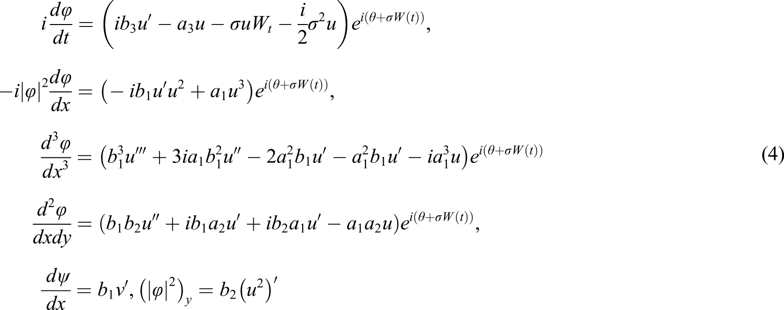
Integrating equation (6) once with respect to ς to obtain

3 b_{1} v + b_{2} u^{2} = c

(7)

where c is an integration constant. For simplicity here, we put c = 0, hence equation (7) becomes

v = \frac{- b_{2}}{3 b_{1}} u^{2}

(8)

Substituting equation (8) into (5), we have the following traveling wave equation

u^{″} - Θ_{1} u^{3} - Θ_{2} u = 0

(9)

where

Θ_{1} = \frac{1}{3 b_{1}^{2}} and Θ_{2} = \frac{a_{3} + a_{1} a_{2} + a_{1}^{3}}{b_{1} b_{2} - 3 a_{1} b_{1}^{2}}

(10)

We note that when Θ₂ is negative, then equation (9) adopts a periodic solution (see for instance Refs. 44,45).

The exact solutions of stochastic HMs

In this section, we implement three different methods as He’s semi-inverse method, sin–cosine method, and Riccati–Bernoulli sub-ODE method, respectively, to obtain the solutions of equation (9). After then, we have the stochastic exact solution of the HMs (1–2).

He’s semi-inverse method

The first method we are using to seek the exact solution of the HMs (1–2) is He’s semi-inverse method. The following variational formulation can be constructed from equation (9) by using He’s semi-inverse method mentioned in Refs. 46–48 as

J (u) = \int_{0}^{\infty} {\frac{1}{2} {(u^{'})}^{2} + \frac{1}{4} Θ_{1} u^{4} + \frac{1}{2} Θ_{2} u^{2}} d ς

(11)

We suppose the solitary wave solution of equation (9) according to Ref. 49 takes the form

u (ς) = K sech (ς)

(12)

where K is an unknown constant. Substituting equation (12) into (11), we get

\begin{array}{l} J = \int_{0}^{\infty} [\frac{K^{2}}{2} {sech}^{2} (ς) {tanh}^{2} (ς) - \frac{K^{4}}{4} Θ_{1} {sech}^{4} (ς) + \frac{K^{2}}{2} Θ_{2} {sech}^{2} (ς)] d ς \\ = \frac{K^{2}}{6} - \frac{K^{4}}{6} Θ_{1} + \frac{K^{2}}{2} Θ_{2} \end{array}

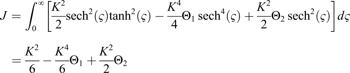
Differentiating J with respect to K and putting $(\partial J / \partial K) = 0$

\frac{\partial J}{\partial K} = \frac{1}{3} (1 + 3 Θ_{2}) K - \frac{2 Θ_{1}}{3} K^{3} = 0

(13)

We get by solving equation (13)

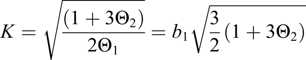
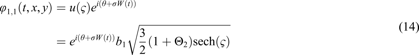
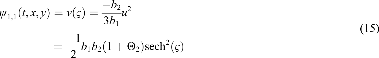
K = \sqrt{\frac{(1 + 3 Θ_{2})}{2 Θ_{1}}} = b_{1} \sqrt{\frac{3}{2} (1 + 3 Θ_{2})}

Hence, the solution of equation (9) is

u (ς) = b_{1} \sqrt{\frac{3}{2} (1 + 3 Θ_{2}) sech (ς)}

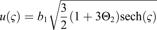
Now, the exact solution of the HMs (1–2) is

\begin{array}{l} φ_{1,1} (t, x, y) = u (ς) e^{i (θ + σ W (t))} \\ = e^{i (θ + σ W (t))} b_{1} \sqrt{\frac{3}{2} (1 + Θ_{2}) sech (ς)} \end{array}

(14)

and

\begin{array}{l} ψ_{1,1} (t, x, y) = v (ς) = \frac{- b_{2}}{3 b_{1}} u^{2} \\ = \frac{- 1}{2} b_{1} b_{2} (1 + Θ_{2}) {sech}^{2} (ς) \end{array}

(15)

Analogously, we can take the solution in the following form

u (ς) = K {sech}^{2} (ς), u (ς) = K csch (ς), u (ς) = K tanh (ς) and u (ς) = K coth (ς)

to get different forms of exact solutions of the HMs (1–2).

Sine–Cosine method

In this subsection, we use the sine–cosine method to get the solitary wave solutions of equation (9) and consequently the exact solution of the HMs (1–2). According to Refs. 14–16, let the solution u of equation (9) take the form

u (ς) = α Y^{m}

(16)

where

Y = \sin (λ ζ) or Y = \cos (λ ζ)

(17)

Substituting equation (16) into (9), we have

- α λ^{2} [- m^{2} Y^{m} + m (m - 1) Y^{m - 2}] - Θ_{1} α^{3} Y^{3 m} - Θ_{2} α Y^{m} = 0

Rewriting the above equation

(Θ_{2} α - α λ^{2} m^{2}) Y^{m} + m (m - 1) α λ^{2} Y^{m - 2} + Θ_{1} α^{3} Y^{3 m} = 0

(18)

Balancing the term of Y in equation (18), we get

m - 2 = 3 m \Rightarrow m = - 1

(19)

Substituting equation (19) into (18)

(Θ_{2} α - α λ^{2}) Y^{- 1} + (Θ_{1} α^{3} + 2 α λ^{2}) Y^{- 3} = 0

(20)

Equating each coefficient of Y⁻¹ and Y⁻³ to zero, we obtain

Θ_{2} α - α λ^{2} = 0

(21)

and

Θ_{1} α^{3} + 2 α λ^{2} = 0

(22)

By solving these equations, we get

λ = \pm \sqrt{Θ_{2}} and α = \pm \sqrt{\frac{- 2 Θ_{2}}{Θ_{1}}}

(23)

Using equation (10), we have

λ = \pm \sqrt{Θ_{2}} and α = \pm \sqrt{- 6 b_{1}^{2} Θ_{2}}

(24)

There are two cases depend on Θ₂:

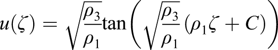
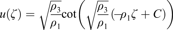
First case: If Θ₂ > 0, then the solitary wave solution takes the form

u (ς) = \pm i \sqrt{6 b_{1}^{2} Θ_{2}} \sec (\sqrt{Θ_{2}} ς) or u (ς) = \pm i \sqrt{6 b_{1}^{2} Θ_{2}} csc (\sqrt{Θ_{2}} ς)

In this case, the exact solution of the stochastic HMs (1–2) takes the form

φ_{1,1} (t, x, y) = \pm i \sqrt{6 b_{1}^{2} Θ_{2}} \sec [\sqrt{Θ_{2}} ς] e^{i (θ + σ W (t))}

(25)

ψ_{1,1} (t, x, y) = 2 b_{1} b_{2} Θ_{2} \sec^{2} [\sqrt{Θ_{2}} ς]

(26)

φ_{1,2} (t, x, y) = \pm i \sqrt{6 b_{1}^{2} Θ_{2}} csc [\sqrt{Θ_{2}} ς] e^{i (θ + σ W (t))}

(27)

ψ_{1,2} (t, x, y) = 2 b_{1} b_{2} Θ_{2} {csc}^{2} [\sqrt{Θ_{2}} ς]

(28)

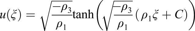
Second case: If Θ₂ < 0, then the solitary wave solution takes the form

u (ς) = \sqrt{- 6 b_{1}^{2} Θ_{2}} sech (\sqrt{- Θ_{2}} ς) or u (ς) = \sqrt{- 6 b_{1}^{2} Θ_{2}} csch (\sqrt{- Θ_{2}} ς)

In this case, the exact solution of the stochastic HMs (1–2) is

φ_{2,1} (t, x, y) = \sqrt{- 6 b_{1}^{2} Θ_{2}} sech [\sqrt{- Θ_{2}} ς] e^{i (θ + σ W (t))}

(29)

ψ_{2,1} (t, x, y) = 2 b_{1} b_{2} Θ_{2} {sech}^{2} [\sqrt{- Θ_{2}} ς]

(30)

φ_{2,2} (t, x, y) = \sqrt{- 6 b_{1}^{2} Θ_{2}} csch [\sqrt{- Θ_{2}} ς] e^{i (θ + σ W (t))}

(31)

ψ_{2,2} (t, x, y) = 2 b_{1} b_{2} Θ_{2}^{2} {csch}^{2} [\sqrt{- Θ_{2}} ς]

(32)

Remark 1

If we put σ = 0 in equations (25)–(32), we obtain the same solutions (see, equations (106), (108), (111), and (113)) stated in Ref. 41.

Riccati–Bernoulli sub-ODE method

Here, we take the following Riccati–Bernoulli equation (9)

u^{'} = ρ_{1} u^{2} + ρ_{2} u + ρ_{3}

(33)

where ρ₁, ρ₂, ρ₃ are constants.

Differentiating equation (33) once with respect to ς, we obtain

u^{″} = 2 ρ_{1} u u^{'} + ρ_{2} u^{'}

utilizing equation (33) gives

u^{″} = 2 ρ_{1}^{2} u^{3} + 3 ρ_{1} ρ_{2} u^{2} + (2 ρ_{1} ρ_{3} + ρ_{2}^{2}) u + ρ_{2} ρ_{3}

(34)

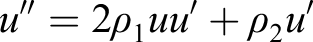
Substituting (34) into (9), we have

(2 ρ_{1}^{2} - Θ_{1}) u^{3} + 3 ρ_{1} ρ_{2} u^{2} + (2 ρ_{1} ρ_{3} + ρ_{2}^{2} - Θ_{2}) u + ρ_{2} ρ_{3} = 0

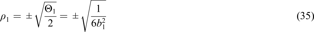
Putting each coefficient of uⁱ(i = 0, 1, 2, 3) equal zero yields system of algebraic equations. We obtain by solving these equations

ρ_{1} = \pm \sqrt{\frac{Θ_{1}}{2}} = \pm \sqrt{\frac{1}{6 b_{1}^{2}}}

(35)

ρ_{2} = 0

(36)

and

ρ_{3} = \frac{Θ_{2}}{2 ρ_{1}} = \pm \frac{\sqrt{6} b_{1} Θ_{2}}{2}

(37)

where we used equation (35). To find the solutions of equation (33), we consider many cases depending on

\frac{ρ_{3}}{ρ_{1}} = \frac{Θ_{2}}{Θ_{1}}

where Θ₁ and Θ₂ are defined in equation (10).

First case: If $(ρ_{3} / ρ_{1}) > 0$ , then the solution of equation (33) is

u (ζ) = \sqrt{\frac{ρ_{3}}{ρ_{1}}} \tan (\sqrt{\frac{ρ_{3}}{ρ_{1}}} (ρ_{1} ζ + C))

u (ζ) = \sqrt{\frac{ρ_{3}}{ρ_{1}}} \cot (\sqrt{\frac{ρ_{3}}{ρ_{1}}} (- ρ_{1} ζ + C))

In this case, the exact solution of the stochastic HMs (1–2) is

φ_{3,1} (t, x, y) = \sqrt{\frac{Θ_{2}}{Θ_{1}}} \tan (\sqrt{\frac{Θ_{2}}{2}} (- ρ_{1} ζ + C)) e^{i (θ + σ W (t))}

(38)

ψ_{3,1} (t, x, y) = - b_{1} b_{2} Θ_{2} \tan^{2} (\sqrt{\frac{Θ_{2}}{2}} (- ρ_{1} ζ + C))

(39)

φ_{3,2} (t, x, y) = \sqrt{\frac{Θ_{2}}{Θ_{1}}} \cot (\sqrt{\frac{Θ_{2}}{2}} (- ρ_{1} ζ + C)) e^{i (θ + σ W (t))}

(40)

ψ_{3,2} (t, x, y) = - b_{1} b_{2} Θ_{2} \cot^{2} (\sqrt{\frac{Θ_{2}}{2}} (- ρ_{1} ζ + C))

(41)

Second case: If $(ρ_{3} / ρ_{1}) < 0$ and $| u | < \sqrt{- (ρ_{3} / ρ_{1})}$ , then the solution of equation (33) is

u (ξ) = \sqrt{\frac{- ρ_{3}}{ρ_{1}}} tanh (\sqrt{\frac{- ρ_{3}}{ρ_{1}}} (ρ_{1} ξ + C))

In this case, the exact solution of the stochastic HMs (1–2) is

φ_{3,3} (t, x, y) = \sqrt{\frac{- Θ_{2}}{Θ_{1}}} tanh (\sqrt{\frac{- Θ_{2}}{2}} (ρ_{1} ξ + C)) e^{i (θ + σ W (t))}

(42)

ψ_{3,3} (t, x, y) = b_{1} b_{2} Θ_{2} {tanh}^{2} (\sqrt{\frac{- Θ_{2}}{2}} (ρ_{1} ξ + C))

(43)

Third case: If $(ρ_{3} / ρ_{1}) < 0$ and $u^{2} > (- ρ_{3} / ρ_{1})$ , then the solution of equation (33) is

u (ξ) = \sqrt{\frac{- ρ_{3}}{ρ_{1}}} coth (\sqrt{\frac{- ρ_{3}}{ρ_{1}}} (ρ_{1} ξ + C))

In this case, the exact solution of the stochastic HMs (1–2) is

φ_{3,4} (t, x, y) = \sqrt{\frac{- Θ_{2}}{Θ_{1}}} coth (\sqrt{\frac{- Θ_{2}}{2}} (ρ_{1} ξ + C)) e^{i (θ + σ W (t))}

(44)

ψ_{3,4} (t, x, y) = b_{1} b_{2} Θ_{2} {coth}^{2} (\sqrt{\frac{- Θ_{2}}{2}} (ρ_{1} ξ + C))

(45)

where Θ₁ and Θ₂ are defined in equation (10).

Remark 2

If we put σ = 0 in equations (38)–(45), we obtain the same solutions (see, equations (93), (95), (100), and (102)) stated in Ref. 41.

Remark 3

We can apply different methods such as the Hirota bilinear method, the Painleve test, the Painleve approach, Weierstrass elliptic function expansion method, the complex hyperbolic function method, the extended trial equation method, the extended tanh method, the improved $tan (ϕ (ρ) / 2)$ -expansion method, the exp(−φ)-expansion method, etc. to get some various solutions. Thus, we can generalize the results found in Refs. 36–43.

The impact of noise on the solutions of HMs

In this section, we show the effect of multiplicative noise on the exact solution of the HMs (1–2). In the following section, we provide some graphical representations to illustrate the behavior of these solutions. We use the MATLAB package to simulate the solution (42) for various σ (noise strength) and for fixed parameters a₁ = 0.9, a₂ = 0, a₃ = 1.4, b₁ = −1.7, b₂ = 0 and b₃ = 3.06 as follows:

In Figure 1, we see that the solution of the HMs (1–2) fluctuates and has a pattern if the noise intensity σ = 0:

Figure 1.

The solution in equation (42) with σ = 0.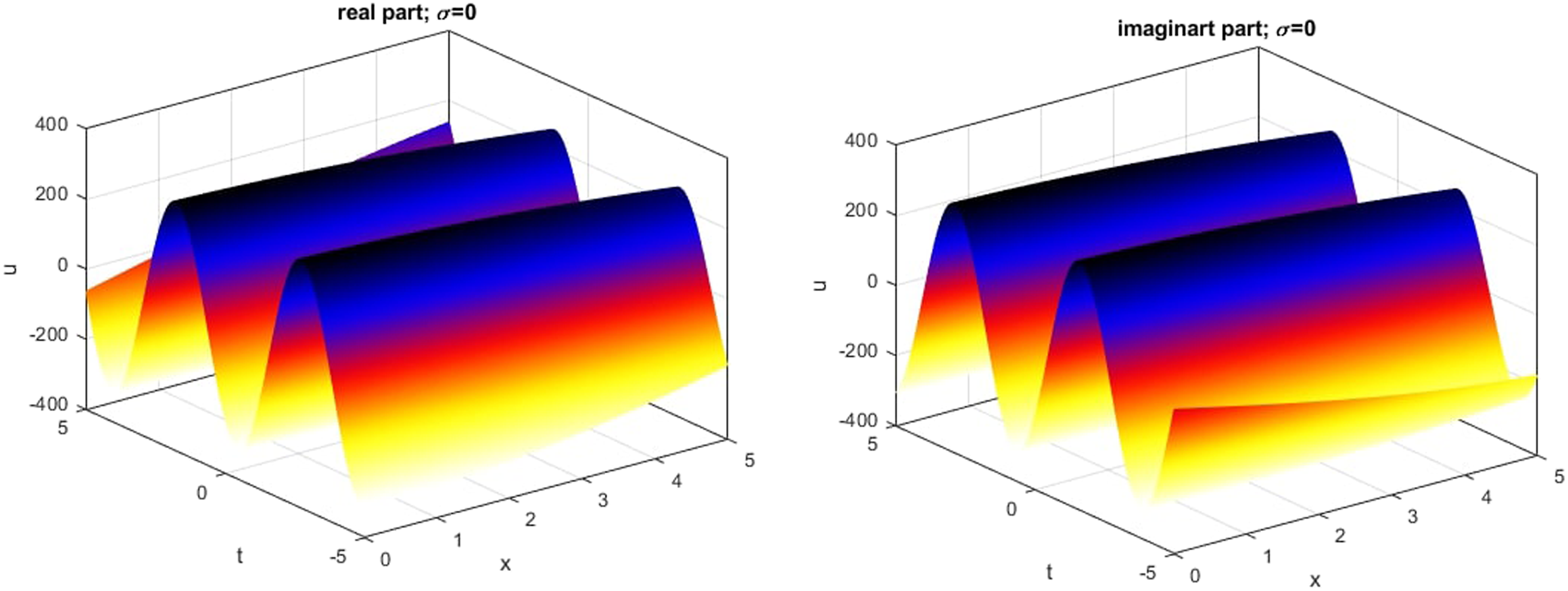

In Figures 2–4, we see that the pattern begins to destroy if the noise intensity σ increases.

Figure 2.

The solution in equation (42) with σ = 1.

Figure 3.

The solution in equation (42) with σ = 3.

Figure 4.

The solution in equation (42) with σ = 5.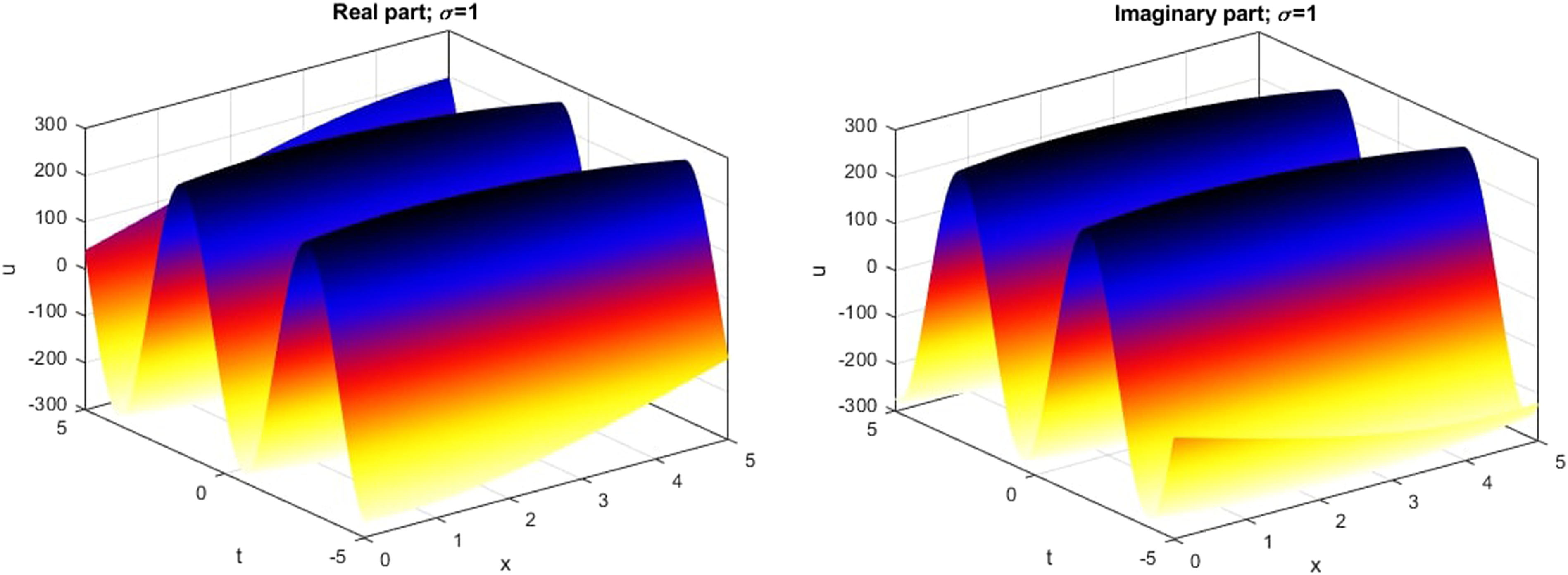

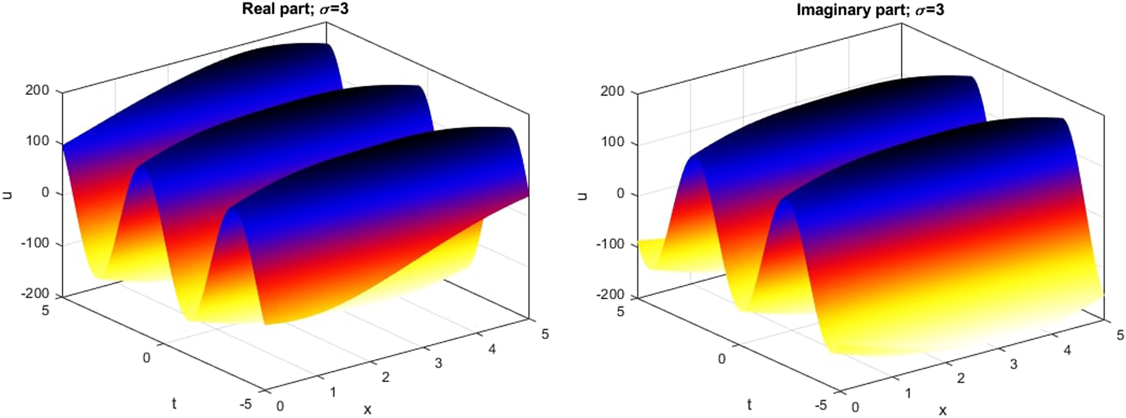
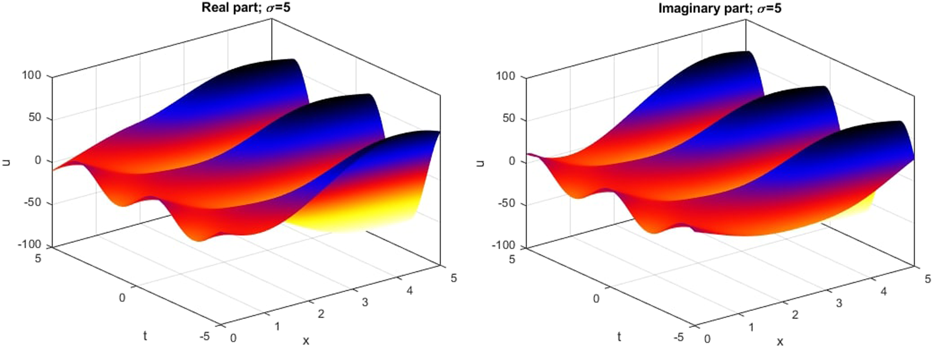
We see that when σ = 0, then the solution u takes the value between −400 and 400 as depicted in Figure 1. Moreover, we see that the values of the solution u begin to decrease and go to zero when the noise increases as seen in Figures 1–4. Also, we note that the blue and yellow color in the pattern indicates the maximum and minimum amplitude of the solution of the given system (1–2).

Figure 5 illustrates the 2D graph corresponding to the solution (42) for σ = 0, 1, 3, 5.

Figure 5.

The picture profile of solution in equation (42).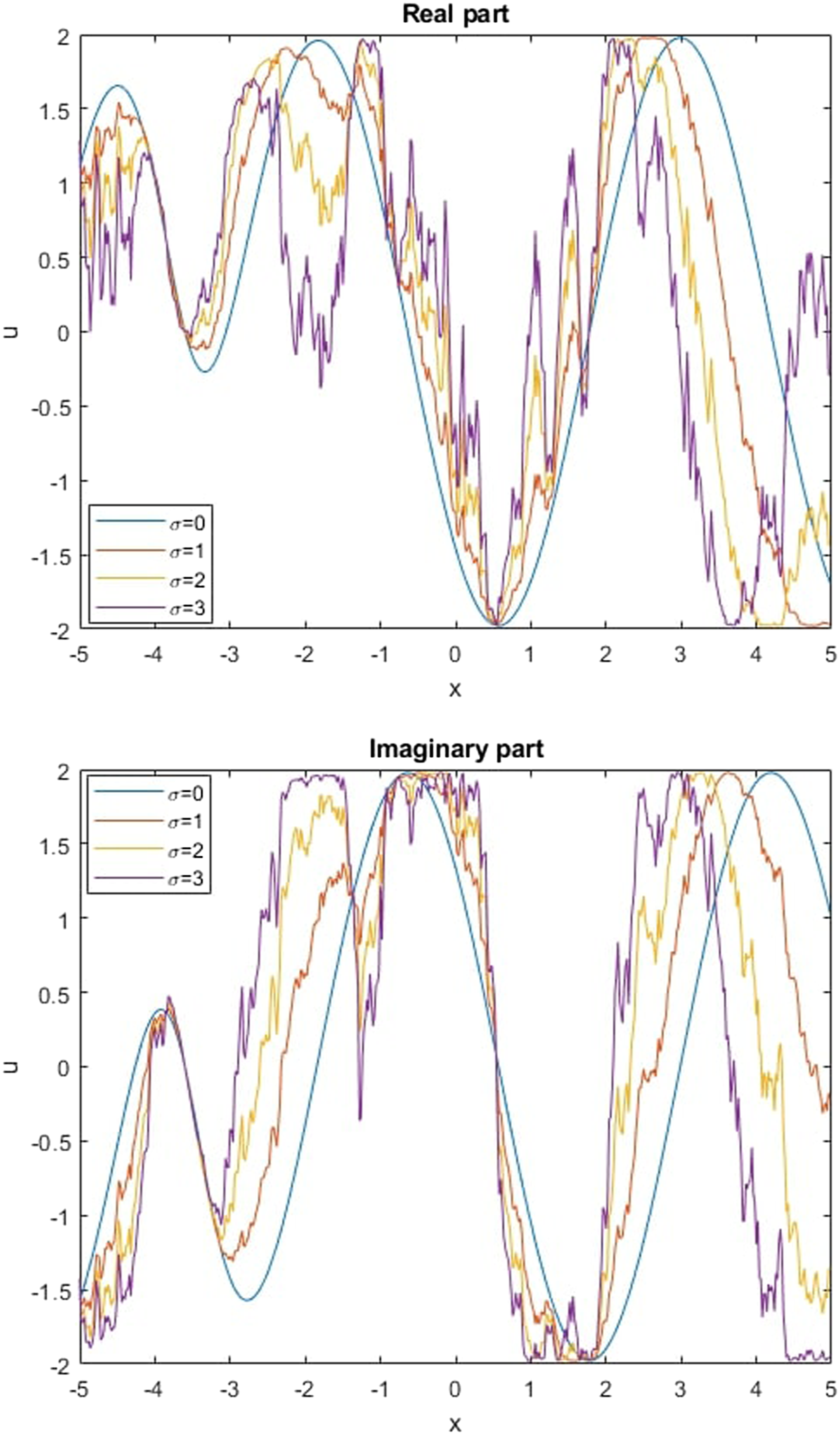

Conclusions

In this article, we obtained various solutions of stochastic exact solution for the stochastic Hirota–Maccari system (1–2) forced in the Itô sense by multiplicative noise. We used three different methods as He’s semi-inverse method, sin–cosine method, and Riccati–Bernoulli sub-ODE method to obtain exact solutions of the stochastic Hirota–Maccari system (1–2). By applying these methods, we extended and improved some results such as the results stated in Ref. 41. Finally, we studied the impact of multiplicative noise on the exact solutions of the Hirota–Maccari system (1–2) by using MATLAB package and we noted that the multiplicative noise in the Itô sense effects on the solutions of the Hirota–Maccari system and it makes the solutions stable around zero.

Footnotes

Declaration of conflicting interests

The author(s) declared no potential conflicts of interest with respect to the research, authorship, and/or publication of this article.

Funding

The author(s) disclosed receipt of the following financial support for the research, authorship, and/or publication of this article: This research has been funded by Scientific Research Deanship at University of Ha’il – Saudi Arabia through project number RG-191207.

ORCID iDs

Wael W. Mohammed

Hijaz Ahmad

References

Khan

Akbar

. The exp(−Φ(ξ))-expansion method for finding travelling wave solutions of Vakhnenko-Parkes equation. Int J Dynamical Syst Differential Equations 2014; 5: 72–83.

Yan

. Abundant families of Jacobi elliptic function solutions of the (2+1)-dimensional integrable Davey-Stewartson-type equation via a new method. Chaos, Solitons & Fractals 2003; 18: 299–309.

. A new approach to nonlinear partial differential equations. Commun Nonlinear Sci Numer Simulation 1997; 2: 230–235.

Yusufoglu

. The variational iteration method for studying the Klein-Gordon equation. Appl Math Lett 2008; 21: 669–674.

Wang

Zhang

. The ()-expansion method and travelling wave solutions of nonlinear evolution equations in mathematical physics. Phys Lett A 2008; 372: 417–423.

Zhang

. New application of the -expansion method. Commun Nonlinear Sci Numer Simul 2009; 14: 3220–3225.

. An approximate solution technique depending on an artificial parameter: a special example. Commun Nonlinear Sci Numer Simulation 1998; 3: 92–97.

El-DibY

. The enhanced homotopy perturbation method for axial vibration of strings. Facta Universitatis, Ser Mech Eng 2021: 1–17. doi:10.22190/FUME210125033H

Yang

X-F

Deng

Z-C

Wei

. A Riccati-Bernoulli sub-ODE method for nonlinear partial differential equations and its application. Adv Difference Equations 2015; 2015: 117–133.

10.

Mohammed

. Approximate solution of the Kuramoto-Shivashinsky equation on an unbounded domain. Chin Ann Math Ser B 2018; 39: 145–162.

11.

Mohammed

. Modulation equation for the stochastic Swift–Hohenberg equation with cubic and quintic nonlinearities on the real line. Mathematics 2020; 6: 1–12.

12.

Hou

Qie

, et al. Hamiltonian-based frequency-amplitude formulation for nonlinear oscillators. Facta Universitatis, Ser Mech Eng 2021: 1–10. doi:10.22190/FUME

13.

Qie

Houa

. The fastest insight into the large amplitude vibration of a string. Rep Mech Eng 2020; 1(2): 1–5.

14.

Wazwaz

. Exact solutions to the double sinh-gordon equation by the tanh method and a variable separated ODE method. Comput Mathematics Appl 2005; 50: 1685–1696.

15.

Wazwaz

A-M

. A sine-cosine method for handlingnonlinear wave equations. Math Computer Model 2004; 40: 499–508.

16.

Yan

. A simple transformation for nonlinear waves. Phys Lett A 1996; 224: 77–84.

17.

Hirota

. Exact solution of the Korteweg-de Vries equation for multiple collisions of solitons. Phys Rev Lett 1971; 27: 1192–1194.

18.

Wazwaz

A-M

. The tanh method: exact solutions of the sine-Gordon and the sinh-Gordon equations. Appl Mathematics Comput 2005; 167: 1196–1210.

19.

Malfliet

Hereman

. The tanh method: I. Exact solutions of nonlinear evolution and wave equations. Physica Scripta 1996; 54: 563–568.

20.

Qie

, et al. On a strong minimum condition of a fractal variational principle. Appl Mathematics Lett 2021; 119: 107199.

21.

. A fractal variational theory for one-dimensional compressible flow in a microgravity space. Fractals 2020; 28(2): 2050024.

22.

Kou

, et al. Fractal oscillation and its frequency-amplitude property. Fractals 2021; 29(4): 2150105.

23.

J-H

. On the fractal variational principle for the Telegraph equation. Fractals 2021; 29: 2150022.

24.

Chunyan Qin

Tian

Shoufu Tian

, et al. Lie symmetry analysis, conservation laws and exact solutions of fourth-order time fractional burgers equation. J Appl Anal Comput 2018; 8: 1727–1746.

25.

Wang

Tian

Qin

, et al. Lie symmetry analysis, conservation laws and analytical solutions of a time-fractional generalized KdV-type equation. J Nonlinear Math Phys 2017; 24: 516–530.

26.

Mohammed

. Fast-diffusion limit for reaction-diffusion equations with degenerate multiplicative and additive noise. J Dyn Differential Equations 2021; 33: 577–592.

27.

Mohammed

. Approximate solutions for stochastic time‐fractional reaction-diffusion equations with multiplicative noise. Math Methods Appl Sci 2021; 44: 2140–2157.

28.

Khan

NAU

Naveed

Mohammed

. Optimal control of nonlocal fractional evolution equations in the α−norm of order (1,2). Adv Difference Equations 2021; 2021: 1–22.

29.

Mohammed

Ahmad

Hamza

, et al. The exact solutions of the stochastic Ginzburg-Landau equation. Results Phys 2021; 23: 103988.

30.

Albosaily

Mohammed

Aiyashi

, et al. Exact solutions of the (2+1)-dimensional stochastic chiral nonlinear Schrödinger equation. Symmetry 2020; 12(11): 1874.

31.

Mohammed

Iqbal

Ali

, et al. Exact solutions of the stochastic new coupled Konno-Oono equation. Results Phys 2021; 21: 103830.

32.

Abdelrhman

Mohammed

Alesemi

, et al. The effect of multiplicative noise on the exact solutions of nonlinear Schrödinger equation. AIMS Mathematics 2021; 6(3): 2970–2980.

33.

Mohammed

Albosaily

Iqbal

, et al. The effect of multiplicative noise on the exact solutions of the stochastic Burgers’ equation. Waves in Random and Complex Media. doi:10.1080/17455030.2021.1905914

34.

Mohammed

El-Morshedy

. The influence of multiplicative noise on the stochastic exact solutions of the Nizhnik-Novikov-Veselov system. Mathematics Comput Simulation 2021; 190: 192–202.

35.

Maccari

. A generalized Hirota equation in 2+1 dimensions. J Math Phys 1998; 39: 6547–6551.

, et al. N-soliton solutions for the (2+1)-dimensional Hirota-Maccari equation in fluids, plasmas and optical fibers. J Math Anal Appl 2011; 378: 519–527.

37.

G-q

Z-b

. The Painlevé test of nonlinear partial differential equations and its implementation using maple. Computer Algebra Geometric Algebra Appl 2005; 3519: 179–190.

38.

Liang

Tang

. Modulational instability and variable separation solution for a generalized (2+1)-dimensional Hirota equation. Chin Phys Lett 2010; 27: 1–4.

39.

Chen

Yan

. The Weierstrass elliptic function expansion method and its applications in nonlinear wave equations. Chaos, Solitons & Fractals 2006; 29: 948–964.

. Complex hyperbolic-function method and its applications to nonlinear equations. Phys Lett A 2006; 355: 32–38.

41.

Wazwaz

. Abundant soliton and periodic wave solutions for the coupled Higgs eld equation, the Maccari system and the Hirota-Maccari system. Physica Scripta 2012; 85: 1–10.

, et al. Explicit solutions of the (2 + 1)-dimensional Hirota-Maccari system arising in nonlinear optics. Int J Mod Phys B 2019; 33: 1950360.

. All exact travelling wave solutions of Hirota equation and Hirota-Maccari system. Optik 2016; 127: 1848–1859.

44.

J-H

El-Dib

. Periodic property of the time-fractional Kundu-Mukherjee-Naskar equation. Results Phys 2020; 19: 103345.

45.

J-H

. Variational principle and periodic solution of the Kundu-Mukherjee-Naskar equation. Results Phys 2020; 17: 103031.

46.

J-H

. Semi-inverse method of establishing generalized variational principles for fluid mechanics with emphasis on turbomachinery aerodynamics. Int J Turbo Jet Engines 1997; 14: 23–28.

47.

J-H

. Variational principles for some nonlinear partial differential equations with variable coefficients. Chaos, Solitons & Fractals 2004; 19: 847–851.

48.

J-H

. Some asymptotic methods for strongly nonlinear equations. Int J Mod Phys B 2006; 20: 1141–1199.

49.

Y-H

L-F

. He's variational method for the Benjamin-Bona-Mahony equation and the Kawahara equation. Comput Mathematics Appl 2009; 58: 2420–2422.

Exact solutions of Hirota–Maccari system forced by multiplicative noise in the Itô sense

Abstract

Keywords

Introduction

Traveling wave eq. for stochastic HMs

The exact solutions of stochastic HMs

He’s semi-inverse method

Sine–Cosine method

Riccati–Bernoulli sub-ODE method

The impact of noise on the solutions of HMs

Conclusions

Footnotes

Declaration of conflicting interests

Funding

ORCID iDs

References