Fast multiline spectral reshaping algorithm for active vibration control

Abstract

Multiline spectral vibration (or noise) is very common in rotating machinery like motor, gearbox, compressor, propeller, etc. Active reshaping of these vibrations is one of the most important branches for active vibration control, which may find application in fields of sound quality control, psychoacoustics, military camouflage, etc. The traditional filtered-reference LMS is the most popular structure for multiline spectral reshaping control. However, with the increase of spectral lines, vibration sources and observation points (feedback channels), the traditional structure will have extremely heavy computational complexity, especially for the system whose dynamic of secondary path is complex, since it requires two long filters for every single spectral line and secondary path to adjust the reference signals. In this study, we propose a fast-multiline spectrum reshaping algorithm for active vibration control. We first construct an equivalent system of the traditional multiline spectrum reshaping algorithm by introducing two extra control branches, which is able to improve the convergence property of the system. Then, we generate a group of pre-phase-scheduled reference signals using the phase information at certain frequencies of the secondary paths instead of using filters. Afterwards, we conduct a theoretical analysis of computational complexity of multiline spectrum reshaping and fast multiline spectrum reshaping algorithms. Finally, we carried out two case studies based on the FEMilS test-bed to verify the effectiveness of the proposed algorithm. The results show that the proposed algorithm performs an accurate residual vibration control with uniformed convergence speed and reduced computational complexity.

Introduction

Active vibration control (AVC) technology is one of the most important technologies in controlling the unwanted vibration. It adds secondary vibration source to the control system and cancels the unwanted vibration based on the principle of superposition.^1–7 Generally, the aim of AVC system is to suppress the unwanted vibration as much as possible. However, with the development of the technology, there is a new branch called active vibration reshaping arising,^8,9 which may find application in fields of sound quality control, psychoacoustics, military camouflage, wearable device, etc. In vehicle engineering, certain components of the engine’s noise are expected to be reserved as an auditory feedback for safety purpose. ¹⁰ Residual vibration in warships is expected to be reshaped according to the demands of comfort or stealth.

The most popular algorithm for active reshaping of line spectral noise is called active noise equalizer (ANE).^11–13 The ANE actually extended the application of narrow-band filtered-reference LMS algorithm ¹⁴ by feeding a pseudo-error signal instead of the real residual error back to the LMS algorithm. Studies related to line spectral reshaping algorithms include frequency domain ANE algorithm, ¹⁵ multi-channel spectral reshaping,^8,16 frequency mismatch in line spectral reshaping algorithm, ¹⁷ etc. The line spectral reshaping algorithm was first introduced to sound quality control by Kuo^18,19 by considering some practical problems like convergence improvement. Gonzalez et al.¹⁶ proposed the common-error line spectral reshaping algorithm for less computational complexity and overshoot, and a multi-channel extension of such algorithm was implemented inside a wooden listening room. De Oliveira et al. ²⁰ proposed a line-spectral reshaping algorithm called NEX–LMS algorithm for ASQC, and the experimental validation was performed with the aid of a vehicle mockup excited by engine noise.

Although ANE has been a very popular and important residual noise reshaping method, it is sensitive to the SP modeling error.^21,22 Rees and Elliott²¹ proposed a phase-scheduled command FXLMS (PSC–FXLMS) algorithm to avoid such problem. Liu et al.²³ proposed an algorithm, called enhance ANE, which is able to directly tuning the residual amplitude of the line spectrum. They also proposed an amplitude and phase control algorithm for line spectrum reshaping. ⁹ For filtered-reference algorithm, with the increase of vibration sources and observation points, the computational complexity will increase dramatically. ²⁴ Since the ANE algorithm has the same structure with filtered-reference algorithm, it requires two filters for every spectral line and every local source, which may lead to extremely large computational complexity when number of spectral lines and external sources is large.

In this study, we aim at troubleshooting the computational complexity problem of multiline, multi-source, multi-input and multi-output spectral reshaping algorithm. A fast-active reshaping algorithm for multiline spectrum has been proposed. The proposed algorithm is finally verified on the benchmark FEMilS test-bed. This paper is organized as follows: ‘Algorithm formulation’ section gives an introduction of proposed algorithm using matrix representation. ‘Test on finite element model’ section conducts different case studies testing the performance of the algorithm; last section is a brief conclusion.

Algorithm formulation

MLSR algorithm

The most popular MLSR algorithm is shown in Figure 1. It is a multiple source, multiple frequency, multiple input and multiple output (MSMF–MIMO) extension of the ANE algorithm. As shown in Figure 1, suppose there is J external source, M local source and K error sensor, in which the ith external source contains $I_j$ frequency component. All the frequencies of all the sources can be combined into a column vector to generate reference signals, i.e.

$${\mathbf{\omega }}_{\text{ref}}(I)={\left\{{\omega }_{\text{ref}}(i)\right\}}^{\text{T}},\hspace{1em}i=1,2,\dots ,I$$

(1)

where $I={\displaystyle {\sum }_{j=1}^J{I}_j}$ is the number of total frequency components. Accordingly, two reference vectors can be defined as

$$\begin{array}{l}{\mathbf{x}}_{\text{c}}(n;I)={\left\{x_{\text{c}}(n;i)\right\}}^{\text{T}}={\left\{\cos \left[{\omega }_{\text{ref}}(i)\cdot n\right]\right\}}^{\text{T}},\hspace{1em}i=1,2,\dots ,I\\ {\mathbf{x}}_{\text{s}}(n;I)={\left\{x_{\text{s}}(n;i)\right\}}^{\text{T}}={\left\{\sin \left[{\omega }_{\text{ref}}(i)\cdot n\right]\right\}}^{\text{T}},\hspace{1em}i=1,2,\dots ,I\end{array}$$

(2)

where n denotes the discrete-time series which can be viewed as an independent variable, and I can be viewed as a parameter. For each local source and each frequency component, there will be two coefficients in the controller. Thus, the controller coefficients can be defined in two matrixes, i.e.

$$\begin{array}{c}{\mathbf{W}}_{\text{c}}(n;I,K)=\left[w_{\text{c}}(n;i,k)\right],\hspace{1em}i=1,2,\dots ,I,k=1,2,\dots ,K\\ {\mathbf{W}}_{\text{s}}(n;I,K)=\left[w_{\text{s}}(n;i,k)\right],\hspace{1em}i=1,2,\dots ,I,k=1,2,\dots ,K\end{array}$$

(3)

where $w_{\text{c}}(n;i,k)$ and $w_{\text{s}}(n;i,k)$ denote the controller coefficients for the ith frequency component and kth local source. MLSR system makes use of equalization parameters for the residual spectrum reshaping. The equalization parameters can be defined as a (I × I) dimensional diagonal matrix, i.e.

$$\mathbf{\Gamma }(I,I)=\text{diag}\left\{\gamma (i)\right\},\hspace{1em}i=1,2,\dots ,I$$

(4)

where $\gamma (i)$ denotes the equalization parameter of the ith frequency component. MLSR system has two branches, in which the one, called cancelling branch, is used to drive the local sources and the other one, called equalization branch, is used to build pseudo-error signal. According to equations (2) to (4), the output of the cancelling and equalization branch of MLSR can be expressed as

$${\mathbf{y}}_{\text{ca}}(n;K)={\mathbf{W}}_{\text{c}}^{\text{T}}(n;I,K)\left[\mathbf{I}(I,I)-\mathbf{\Gamma }(I,I)\right]{\mathbf{x}}_{\text{c}}(n;I)+{\mathbf{W}}_{\text{s}}^{\text{T}}(n;I,K)\left[\mathbf{I}(I,I)-\mathbf{\Gamma }(I,I)\right]{\mathbf{x}}_s(n;I)$$

(5)

and

$${\mathbf{y}}_{\text{ba}}(n;K)={\mathbf{W}}_{\text{c}}^{\text{T}}(n;I,K)\mathbf{\Gamma }(I,I){\mathbf{x}}_{\text{c}}(n;I)+{\mathbf{W}}_{\text{s}}^{\text{T}}(n;I,K)\mathbf{\Gamma }(I,I){\mathbf{x}}_s(n;I)$$

(6)

Figure 1.

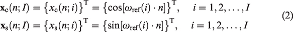
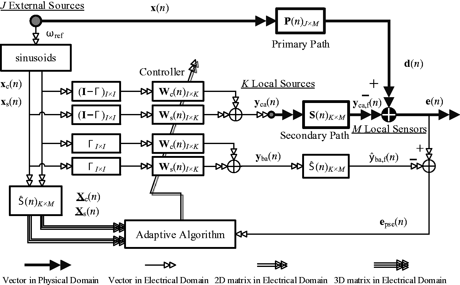
Diagram of classical MLSR algorithm.

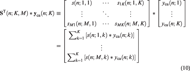
The secondary path (SP) matrix is defined to be

$$\mathbf{S}(n;K,M)\equiv \left[s(n;k,m)\right],\hspace{1em}k=1,2,\dots ,K,\hspace{1em}m=1,2,\dots ,M$$

(7)

where $s(n;k,m)$ denotes the SP from kth secondary source to mth error sensor. The real-error signals are superposition of primary noises and secondary noises, i.e.

$$\mathbf{e}(n;M)=\mathbf{d}(n;M)-{\mathbf{S}}^{\text{T}}(n;K,M)\ast {\mathbf{y}}_{\text{ca}}(n;K)$$

(8)

where $\mathbf{e}(n;M)$ denotes real-error signal

$$\mathbf{d}(n;M)={\mathbf{P}}^{\text{T}}(n;J,M)\mathbf{x}(n;J)$$

(9)

denotes primary noise signal and * denotes linear convolution. The calculation of linear convolution between matrixes is defined to be the same as matrix, i.e.

$$\begin{array}{l}{\mathbf{S}}^{\text{T}}(n;K,M)\ast {\mathbf{y}}_{\text{ca}}(n;K)\equiv \left[\begin{array}{ccc}s(n;1,1)& \cdots & s_{1K}(n;1,K)\\ ⋮& \ddots & ⋮\\ s_{M1}(n;M,1)& \cdots & s_{MK}(n;M,K)\end{array}\right]*\left[\begin{array}{c}{y}_{\text{ca}}(n;1)\\ ⋮\\ y_{\text{ca}}(n;K)\end{array}\right]\\ =\left[\begin{array}{c}{\displaystyle {\sum }_{k=1}^K\left[s(n;1,k)*y_{\text{ca}}(n;k)\right]}\\ ⋮\\ {\displaystyle {\sum }_{k=1}^K\left[s(n;M,k)*y_{\text{ca}}(n;k)\right]}\end{array}\right]\end{array}$$

(10)

The pseudo-error vector is used to feedback the adaptive algorithm for the controller coefficients updating. It can be expressed as

$${\mathbf{e}}_{\text{pse}}(n;M)=\mathbf{e}(n;M)-{\widehat{\mathbf{S}}}^{\text{T}}(n;K,M)\ast {\mathbf{y}}_{\text{ba}}(n;K)$$

(11)

where $\widehat{\mathbf{S}}(n;K,M)$ is the model of $\mathbf{S}(n;K,M)$ . The filtered reference signals are also required for the controller coefficients updating. They are (K × M × I) dimensional matrix, i.e.

$$\begin{array}{c}{\underset{¯}{\mathbf{X}}}_{\text{c}}(n;K,M,I)=\widehat{\mathbf{S}}(n;K,M)\ast {\mathbf{x}}_{\text{c}}(n;I)\\ {\underset{¯}{\mathbf{X}}}_{\text{c}}(n;K,M,I)=\widehat{\mathbf{S}}(n;K,M)\ast {\mathbf{x}}_{\text{s}}(n;I)\end{array}$$

(12)

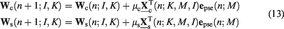
According to the stochastic descent method, the updating equation of the controller coefficient can be expressed as

$$\begin{array}{l}{\mathbf{W}}_{\text{c}}(n+1;I,K)={\mathbf{W}}_{\text{c}}(n;I,K)+{\mu }_{\text{c}}{\underset{¯}{\mathbf{X}}}_{\text{c}}^{\text{T}}(n;K,M,I){\mathbf{e}}_{\text{pse}}(n;M)\\ {\mathbf{W}}_{\text{s}}(n+1;I,K)={\mathbf{W}}_{\text{s}}(n;I,K)+{\mu }_{\text{s}}{\underset{¯}{\mathbf{X}}}_{\text{s}}^{\text{T}}(n;K,M,I){\mathbf{e}}_{\text{pse}}(n;M)\end{array}$$

(13)

where ${\underset{¯}{\mathbf{X}}}_{\text{c}}^{\text{T}}(n;K,M,I)$ is transpose of ${\underset{¯}{\mathbf{X}}}_{\text{c}}(n;K,M,I)$ and is a (I × K × M) dimensional matrix.

The proposed FMLSR algorithm

The traditional MLSR algorithm is based on filtered-reference LMS structure. There are two drawbacks. One is that there must be two filters for every single spectral line and every SP, so if the number of spectral line and SPs is large, the computational complexity will be very high. The other drawback is that the filter will tune the amplitude of the reference signal, leading to uneven in convergence between different spectral lines.

In this paper, we proposed a fast-multiline spectrum reshaping (FMLSR) algorithm, as shown in Figure 2. Except for the canceling branch ${\mathbf{y}}_{\text{ca}}(n)$ and balance branch ${\mathbf{y}}_{\text{ba}}(n)$ in the traditional structure, two new cancelling branches, i.e. estimated canceling branch ${\widehat{\mathbf{y}}}_{\text{ca}}(n)$ and phase-scheduled canceling branch ${\widehat{\mathbf{y}}}_{\text{ca,ph}}(n)$ are introduced. The adaptive algorithm tunes the controller in the phase-scheduled canceling branch, and the controllers in original canceling branch and balance branch are the copy of the updated controller. If we use an FIR filter to model the SP, the three-dimensional matrix of SP model in time-domain can be expressed as

$$\underset{¯}{\widehat{\mathbf{S}}}(n;L,M,K)={\left\{s(n;l,m,k)\right\}}^{\text{T}},\hspace{1em}l=1,2,\dots ,L;\hspace{1em}m=1,2,\dots ,M;\hspace{1em}k=1,2,\dots ,K$$

(14)

where L is the length of the FIR filter. The transfer function of the SP matrix in z-domain can be expressed as

$$\widehat{\mathbf{S}}(z,n,L;M,K)={\displaystyle \sum _{l=1}^L\left[\widehat{\mathbf{S}}(n,l;M,K)\cdot z^{-(l-1)}\right]}$$

(15)

Figure 2.

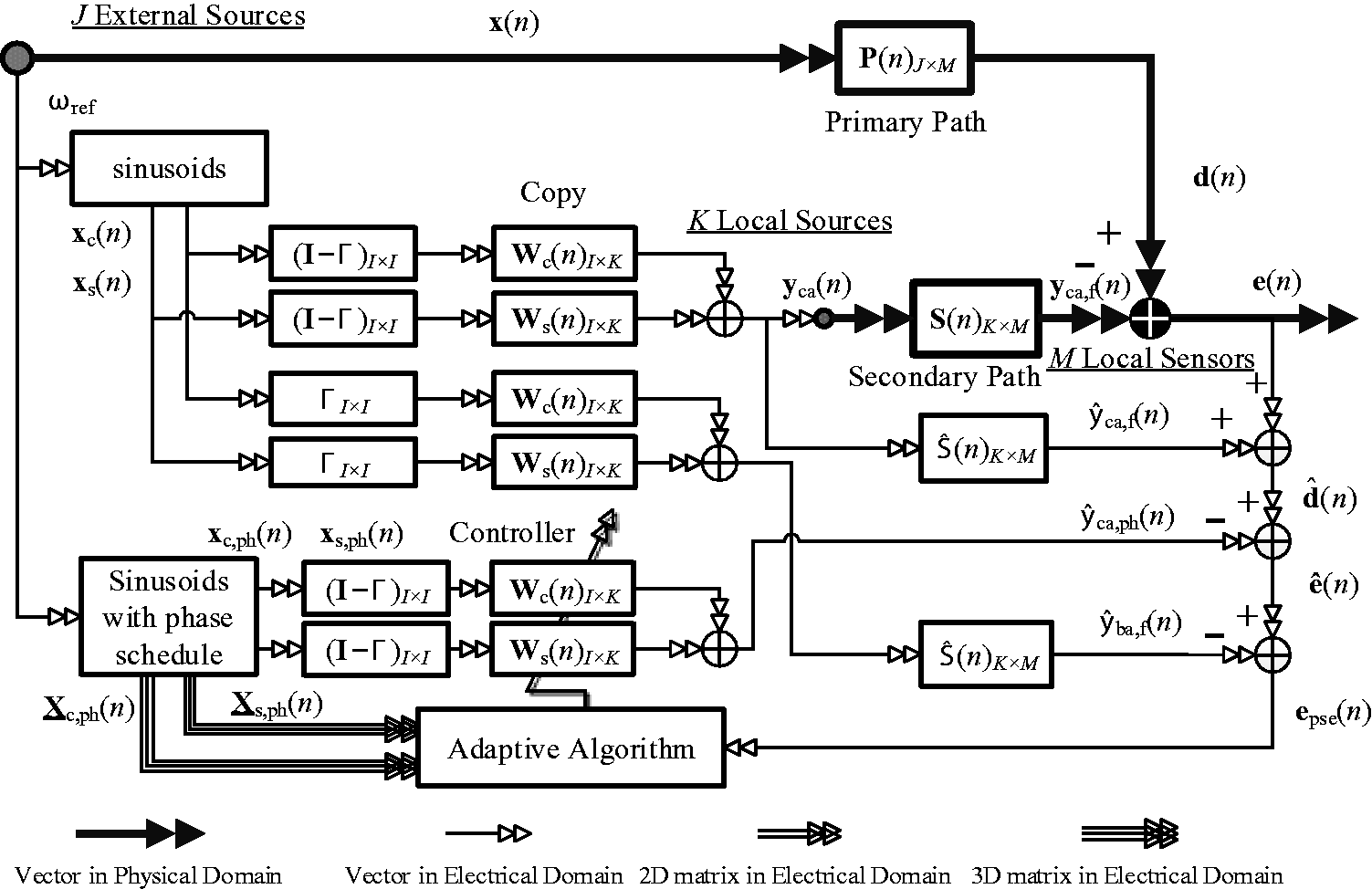
The proposed FMLSR algorithm.

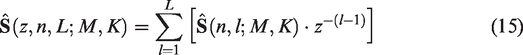
If L is large enough, the identified system will not relate to L. Thus, it cannot be regarded as a parameter. Accordingly, the system in z-domain can be further written as

$$\widehat{\mathbf{S}}(z,n;M,K)={\displaystyle \sum _{l=1}^L\left[\widehat{\mathbf{S}}(n,l;M,K)\cdot z^{-(l-1)}\right]}$$

(16)

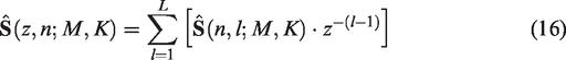
The transfer function in DFT domain is

$$\widehat{\mathbf{S}}(u,n;M,K)={\displaystyle \sum _{l=1}^L\left[\widehat{\mathbf{S}}(n,l;M,K)\cdot e^{-j2\pi lu/L}\right]}$$

(17)

where u denotes discrete frequency. Thus, the phase of the SP model is

$$\mathbf{\Phi }(u,n;M,K)\text{\hspace{0.17em}=\hspace{0.17em}}{\tan }^{-1}\frac{\mathrm{Im}\left[\widehat{\mathbf{S}}(u,n;M,K)\right]}{\mathrm{Re}\left[\widehat{\mathbf{S}}(u,n;M,K)\right]}$$

(18)

and the phase at every reference frequency is

$$\varphi (i,n,m,k)={\varphi (u,n,m,k)|}_{u={\omega }_{\text{r}}(i)},\hspace{1em}i=1,2,\dots ,I$$

(19)

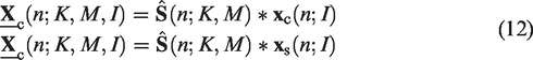
Thus, the reference signal vectors for phase scheduled canceling branch are

$$\begin{array}{c}{\mathbf{x}}_{\text{c,ph}}(n;I)={\left\{x_{\text{c,ph}}(n;i)\right\}}^{\text{T}}={\left\{\cos \left[{\omega }_{\text{ref}}(i)\cdot n+\varphi (i)\right]\right\}}^{\text{T}},\hspace{1em}i=1,2,\dots ,I\\ {\mathbf{x}}_{\text{s,ph}}(n;I)={\left\{x_{\text{s,ph}}(n;i)\right\}}^{\text{T}}={\left\{\sin \left[{\omega }_{\text{ref}}(i)\cdot n+\varphi (i)\right]\right\}}^{\text{T}},\hspace{1em}i=1,2,\dots ,I\end{array}$$

(20)

and the reference signal matrix used for adaptive algorithm is

$$\begin{array}{l}{\underset{¯}{\mathbf{X}}}_{\text{c,ph}}(n;I,M,K)=\left[\cos \left[\omega (i)\cdot n+\varphi (n;i,k,m)\right]\right],\hspace{1em}i=1,2,\dots ,I;\hspace{1em}m=1,2,\dots ,M;\hspace{1em}k=1,2,\dots ,K\\ {\underset{¯}{\mathbf{X}}}_{\text{s,ph}}(n;I,M,K)=\left[\sin \left[\omega (i)\cdot n+\varphi (n;i,k,m)\right]\right],\hspace{1em}i=1,\hspace{1em}2,\dots ,I;\hspace{1em}m=1,2,\dots ,M;\hspace{1em}k=1,2,\dots ,K\end{array}$$

(21)

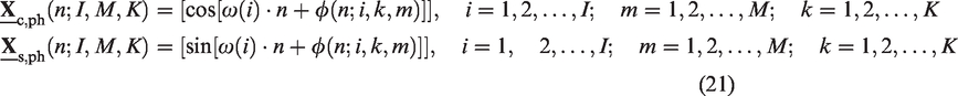
According to Figure 2 and the definitions before, the output of the phase scheduled canceling branch is

$${\mathbf{y}}_{\text{ca,ph}}(n;K)={\mathbf{W}}_{\text{c}}^{\text{T}}(n;I,K)\left[\mathbf{I}(I,I)-\mathbf{\Gamma }(I,I)\right]{\mathbf{x}}_{\text{c},ph}(n;I)+{\mathbf{W}}_{\text{s}}^{\text{T}}(n;I,K)\left[\mathbf{I}(I,I)-\mathbf{\Gamma }(I,I)\right]{\mathbf{x}}_{s,ph}(n;I)$$

(22)

and the filtered signal of canceling and balance branches are

$$\begin{array}{c}{\widehat{\mathbf{y}}}_{\text{ca,f}}(n;M)=\widehat{\mathbf{S}}(n;M,K)\text{*}{\mathbf{y}}_{\text{ca}}(n;K)\\ {\mathbf{y}}_{\text{ca,f}}(n;M)=\mathbf{S}(n;M,K)\text{*}{\mathbf{y}}_{\text{ca}}(n;K)\\ {\widehat{\mathbf{y}}}_{\text{ba,f}}(n;M)=\widehat{\mathbf{S}}(n;M,K)\text{*}{\mathbf{y}}_{\text{ba}}(n;K)\end{array}$$

(23)

Thus, the estimated primary noise is

$$\widehat{\mathbf{d}}(n;M)=\mathbf{e}(n;M)+{\widehat{\mathbf{y}}}_{\text{ca,f}}(n;M)$$

(24)

the estimated real-error is

$$\widehat{\mathbf{e}}(n;M)=\widehat{\mathbf{d}}(n;M)-{\widehat{\mathbf{y}}}_{\text{ca,ph}}(n;M)$$

(25)

and the pseudo-error signal is

$${\mathbf{e}}_{\text{pse}}(n;M)=\widehat{\mathbf{e}}(n;M)-{\widehat{\mathbf{y}}}_{\text{ba,f}}(n;M)$$

(26)

When the system is converging, the pseudo-error is supposed to approach zero. So, the real residual error is

$$\begin{array}{l}\mathbf{e}(\infty ,M)=\widehat{\mathbf{S}}(n;M,K)\text{*}{\mathbf{y}}_{\text{ba}}(\infty ,M)\\ =\widehat{\mathbf{S}}(n;M,K)\text{*}\left[{\mathbf{W}}_{\text{c}}^{\text{T}}(\infty ;I,K)\mathbf{\Gamma }(I,I){\mathbf{x}}_{\text{c}}(n;I)+{\mathbf{W}}_{\text{s}}^{\text{T}}(\infty ;I,K)\mathbf{\Gamma }(I,I){\mathbf{x}}_s(n;I)\right]\end{array}$$

(27)

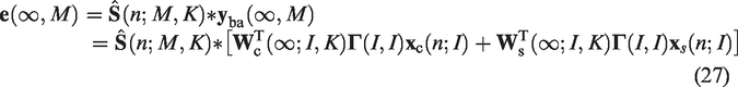
Now, from equation (27), the controller coefficients satisfy the equation

$$\begin{array}{l}\widehat{\mathbf{S}}(n;M,K)\text{*}\left[{\mathbf{W}}_{\text{c}}^{\text{T}}(\infty ;I,K)\mathbf{\Gamma }(I,I){\mathbf{x}}_{\text{c}}(n;I)+{\mathbf{W}}_{\text{s}}^{\text{T}}(\infty ;I,K)\mathbf{\Gamma }(I,I){\mathbf{x}}_s(n;I)\right]\\ +\mathbf{S}(n;M,K)\text{*}\left[{\mathbf{W}}_{\text{c}}^{\text{T}}(n)\left(\mathbf{I}(I,I)-\mathbf{\Gamma }(I,I)\right){\mathbf{x}}_{\text{c}}(n;I)+{\mathbf{W}}_{\text{s}}^{\text{T}}(n)\left(\mathbf{I}(I,I)-\mathbf{\Gamma }(I,I)\right){\mathbf{x}}_s(n;I)\right]=d(n;M)\end{array}$$

(28)

If the SP model is exactly equal to the real system, equation (28) reduces to

$$d(n)=\widehat{\mathbf{S}}(n;M,K)\text{*}\left[{\mathbf{W}}_{\text{c}}^{\text{T}}(\infty ;I,K){\mathbf{x}}_{\text{c}}(n;I)+{\mathbf{W}}_{\text{s}}^{\text{T}}(\infty ;I,K){\mathbf{x}}_s(n;I)\right]$$

(29)

Compare equations (27) and (29), the real error is a reshaping of primary noise. By setting the value of the diagonal elements of $\mathbf{\Gamma }(I,I)$ , the relevant frequency component of the primary noise response can be cancelled (γ_i = 0), suppressed (0 < γ_i < 1), remained (γ_i = 1) or enhanced (γ_i > 1).

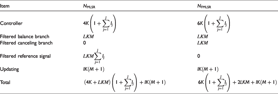
Computational complexity analysis

The computational complexity of MLSR and FMLSR algorithm is discussed by counting the numbers of multipliers required for a single iteration for each algorithm. ²⁴ The results are shown in Table 1. The notations in the table are listed as follows: J denotes the number of external sources (primary sources), K denotes the number of local sources (secondary sources), M denotes the number of error sensors/pseudo-error sensors, $I_j$ denotes the number of spectral lines in the ith external sources, L denotes the length of the FIR filters applied to modeling the SP, $N_{\text{MLSR}}$ and $N_{\text{FMLSR}}$ denote the number of multipliers of MLSR and FMLSR algorithms in a single iteration, respectively. Note that the evaluation in Table 1 does not include the time consumption of the primary path and SP of the controlled system.

Table 1.

Number of multipliers of two algorithms.

Item	$N_{\text{MLSR}}$	$N_{\text{FMLSR}}$
Controller	$4K\left(1+{\displaystyle \sum _{j=1}^J{I}_j}\right)$	$6K\left(1+{\displaystyle \sum _{j=1}^J{I}_j}\right)$
Filtered balance branch	$\mathit{LKM}$	$\mathit{LKM}$
Filtered canceling branch	0	$\mathit{LKM}$
Filtered reference signal	$\mathit{LKM}{\displaystyle \sum _{j=1}^J{I}_j}$	0
Updating	$IK(M+1)$	$IK(M+1)$
Total	$\begin{array}{l}\left(4K+\mathit{LKM}\right)\left(1+{\displaystyle \sum _{j=1}^J{I}_j}\right)+IK(M+1)\end{array}$	$\begin{array}{l}6K\left(1+{\displaystyle \sum _{j=1}^J{I}_j}\right)+2LKM+IK(M+1)\end{array}$

To have a better view of the computational complexity of the different algorithms, we evaluate Table 1 with different number of 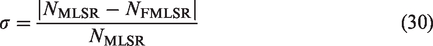$J,K,M,I_j,L$ , and the results are shown in Table 2. The theoretical computation complexity reduction ratio of the FMLSR is defined to be

$$\sigma =\frac{\left|N_{\text{MLSR}}-N_{\text{FMLSR}}\right|}{N_{\text{MLSR}}}$$

(30)

Table 2.

Evaluation of the computational complexity of two algorithms.

I	J	K	M	L	$N_{\text{MLSR}}$	$N_{\text{FMLSR}}$	$\sigma$	I	J	K	M	L	$N_{\text{MLSR}}$	$N_{\text{FMLSR}}$	$\sigma$
4	2	1	1	300	2752	670	0.756	1	2	4	4	300	14,488	9712	0.329
4	2	2	2	300	10,920	2556	0.765	2	2	4	4	300	24,160	9800	0.594
4	2	3	3	300	24,504	5658	0.769	3	2	4	4	300	33,832	9888	0.707
4	2	4	4	300	43,504	9976	0.770	4	2	4	4	300	43,504	9976	0.770
4	2	5	5	300	67,920	15,510	0.771	5	2	4	4	300	53,176	10,064	0.810
4	2	6	6	300	97,752	22,260	0.772	6	2	4	4	300	62,848	10,152	0.838
4	2	7	7	300	133,000	30,226	0.772	7	2	4	4	300	72,520	10,240	0.858
4	2	8	8	300	173,664	39,408	0.773	8	2	4	4	300	82,192	10,328	0.874
4	2	9	9	300	219,744	49,806	0.773	9	2	4	4	300	91,864	10,416	0.886
4	2	10	10	300	271,240	61,420	0.773	10	2	4	4	300	101,536	10,504	0.896
4	1	4	4	300	24,160	9800	0.594	4	2	4	4	100	14,704	3576	0.756
4	2	4	4	300	43,504	9976	0.770	4	2	4	4	200	29,104	6776	0.76
4	3	4	4	300	62,848	10,152	0.838	4	2	4	4	300	43,504	9976	0.770
4	4	4	4	300	82,192	10328	0.874	4	2	4	4	400	57904	13176	0.772
4	5	4	4	300	101,536	10504	0.896	4	2	4	4	500	72304	16376	0.773
4	6	4	4	300	120,880	10680	0.911	4	2	4	4	600	86704	19576	0.77
4	7	4	4	300	140,224	10856	0.922	4	2	4	4	700	101104	22776	0.774
4	8	4	4	300	159,568	11032	0.930	4	2	4	4	800	115504	25976	0.775
4	9	4	4	300	178,912	11208	0.937	4	2	4	4	900	129904	29176	0.775
4	10	4	4	300	198,256	11384	0.942	4	2	4	4	1000	144304	32376	0.775

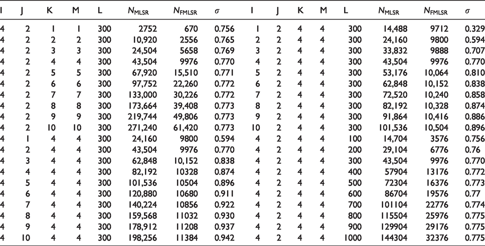
In these calculations, we assume that (1) there is same number of spectral lines in every external source; (2) the filter length of every SPs is the same. It can be seen from Table 2 that (1) the computational complexity of both algorithms increases with the number of channels (K and M) of the control system, and the improvement of the FMLSR is around 75%; (2) the computational complexity of both algorithms increases with the number of spectral lines of the control system, and the improvement of the FMLSR is extremely large in the case that the number of spectral lines is large; (3) the computational complexity of both algorithms increases with the number of external sources of the control system, and the improvement of the FMLSR is extremely large in the case that the number of external sources is large; (4) the computational complexity of both algorithms increases with the filter length of SP, and the improvement of the FMLSR is around 75%. It should be clarified that the evaluation Table 1 still does not include the time consumption of the primary path and SP of the controlled system. Anyhow, we can conclude from the theoretical analysis that the FMLSR can greatly reduce the computational complexity compared to the traditional algorithm.

Test on finite element model

Test-bed

The MLSR and FMLSR algorithms are tested on FEMilS system,^25–27 a benchmark test-bed by embedding the finite element model into the control loop. Particularly, the test is conducted on a variable section cylindrical structure as illustrated in Figure 3. The axial direction of the cylinder is defined as z-axis, and the x–y section is perpendicular to z-axis. The length of the cylinder is 4830 mm, and the maximum radius of the cylinder is 1100 mm. The engineering parameters of the cylindrical structure are listed in Table 3. The geometrical model and its mesh are illustrated using MATLAB. The cylinder is divided into 20 × 16 rectangle elements. Thus, the cylinder has 20 nodes in circumferential direction (x–y section) and 17 nodes in z-axis. Adjacent two elements share two nodes, so there are 340 nodes in cylinder. The baffle has 45 nodes and shares 20 nodes with the cylinder. Thus, the whole structure has 365 nodes. Each node has 6 DOFs, so the total DOFs are 2136, if the cylinder is unconstrained. The xyz translations of each node are considered to be main DOFs of the system, thus reducing the total DOFs to 1068. In Figure 3, the local sources and real-error sensors are placed at node 14 (S1), node 24 (S2), node 285 (S3) and node 295 (S4); the external sources and reference sensors are placed at node 812 (P1) and node 823 (P2).

Figure 3.

The graphical description of the FEMilS test-bed.

Table 3.

Parameters of the FEMilS test-bed.

Item	Symbol	Value
Length of cylinder (m)	l	4.83
Radius of cylinder (m)	r	1.10
Thickness of cylinder (m)	h 1	0.06
Thickness of baffle (m)	h 2	0.06
Modulus of elasticity (Pa)	E	2 × 1011
Poisson’s ratio	ε	0.3
Density (kg/m3)	ρ	7.85 × 103
Modal damping ratio	ξ	0.01
Equivalent mass of actuator (kg)	ma	1
Equivalent damping of actuator (Ns/m)	ca	5.5
Equivalent stiffness of actuator (N/m)	ka	9600
Fixed mass of actuator (kg)	Ma	1.8

The multiline spectral of external sources at P1 and P2 is shown in Figure 4(a) and (b), respectively. P1 contains frequency components of 10, 20, 30, 40 and 50 Hz. P2 contains frequency components of 15, 45 and 75 Hz. The transfer functions of SPs are shown in Figure 5. For MIMO control system, the SPs can be represented using a transfer function matrix, where the elements of the matrix are transfer functions. The curves in Figure 5 represent the elements in the transfer function matrix. The transfer function in the matrix from {S1, S2, S3, S4} to {S1, S2, S3, S4} is shown in Figure 5(a). The transfer function in the matrix from {S1, S2, S3, S4} to {S1, S2, P1, P2} is shown in Figure 5(b). It can be seen that the transfer functions are extremely complex. They require very long filters to model them.

Figure 4.

Multiline spectrum of external sources at P1 (a) and P2 (b).

Figure 5.

Transfer functions between certain points on FEMilS test-bed: (a) transfer function between S1, S2, S3 and S4 and (b) transfer function between S1, S2, P1 and P2.

Case A: Two external sources, two local sources and two error sensors

In case A, two external sources are placed at P1 and P2, and two local sources and two error sensors are placed at S1 and S2. The spectrums of external sources at P1 and P2 are shown in Figure 4(a) and (b), respectively. The frequencies, amplitudes and phases of multiline spectrum at P1 are {10, 20, 30, 40, 50 Hz}, {1, 2, 5, 10, 2 N} and {10°, 20°, 30°, 40°, 50°}, respectively. The frequencies, amplitudes and phases of multiline spectrum at P2 are {15, 45, 75 Hz}, {2, 10, 8 N} and {60°, 70°, 80°}. Besides, there is 20% white noise added to P1 and P2. For the MLSR and FMLSR algorithm, the frequency components of different external sources can be combined together. Thus, the target frequency vector can be expressed as {10, 15, 20, 30, 40, 45, 50, 75 Hz}. The equalization parameters for S1 are set to be {1, 0, 0.4, 0, 1.5, 0, 0.4, 0}, i.e. the amplitudes for the target spectrum are {1 × 10⁻⁶ m, 0 m, 2 × 10⁻⁶ m, 0 m, 3 × 10⁻⁶ m, 0 m, 4 × 10⁻⁶ m, 0 m}. The equalization parameters for S2 are set to be {0, 1.5, 0, 0.2, 0, 1.3, 0.125}, i.e. the amplitudes for the target spectrum are {0 m, 3 × 10⁻⁶ m, 0 m, 2 × 10⁻⁶ m, 0 m, 4 × 10⁻⁶ m, 0 m, 1 × 10⁻⁶ m}. The sampling frequency is 2048 Hz, the sampling time is 12 s and the step-size is 2 × 10⁸.

According to Table 2, there are 10,920 multipliers and 2556 multipliers for MLSR and FMLSR, respectively, for Case A. The proposed FMLSR algorithm will avoid too much filtering operations and reduce the computational complexity by 76.5% theoretically. The time consumption of the simulation in Case A has also been evaluated. In 50 independent trials, the average time consuming of MLSR and FMLSR was 27.60 ± 0.26 s and 7.26 ± 0.04 s, respectively, as shown in Figure 6. It should be clarified that (1) this evaluation was conducted in MATLAB on Windows OS with hardware of Intel Core i7-4790 CPU @3.60 GHz and 16 G RAM; (2) this evaluation contains the time of calculating the in-loop model of FEMilS, function call, etc. It can be seen that both theoretical analysis and numerical simulation verify that the FMLSR is able to reduce the computational complexity dramatically.

Figure 6.

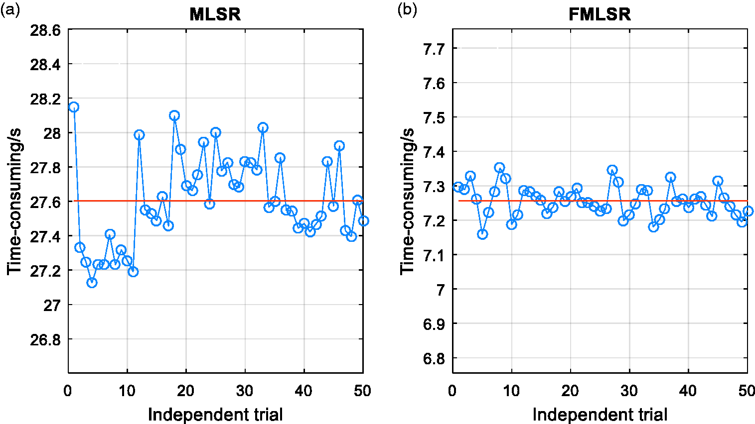
Time consumption of MLSR and FMLSR in Case A.

Figure 7(a) and (b) shows the real-error signals at S1 and S2 when control is ON. Figure 8(a) and (b) shows the pseudo-error signals of S1 and S2 when control is ON. It can be seen that with FMLSR control, the pseudo-error signals approach to zeroes, while the real-error signals approach to a pre-defined signal. Figure 9(a) and (b) shows the spectrum of real-error signal of S1 and S2, respectively, at 10 s when the control is ON and OFF. It can be seen that when the control is ON, the residual spectrum is successfully reshaped according to the target spectrum with a very high accuracy, even though there are different targets spectrum at S1 and S2.

Figure 7.

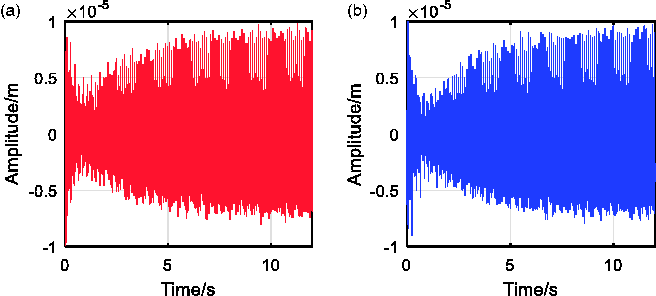
Real-error signal at S1 (a) and S2 (b) in Case A.

Figure 8.

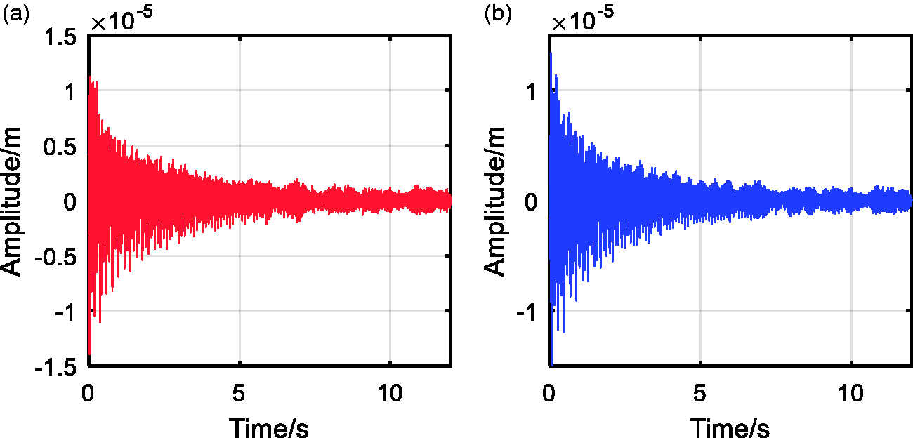
Pseudo-error signal at S1 (a) and S2 (b) in Case A.

Figure 9.

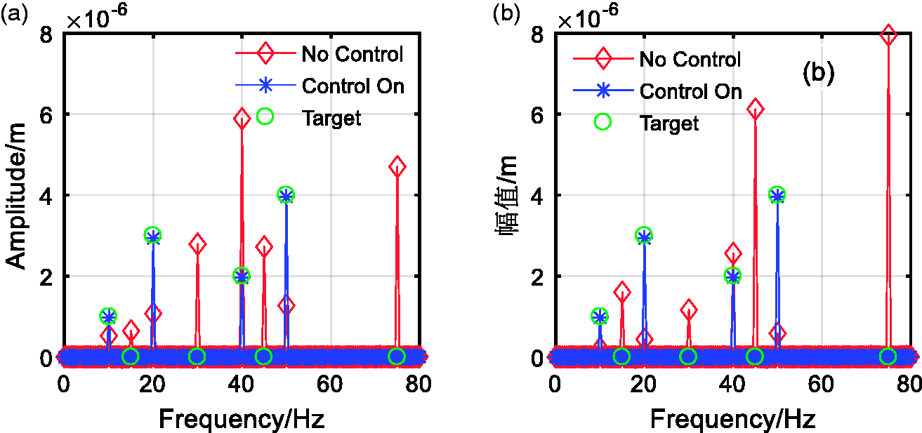
Multiline spectrums at S1 (a) and S2 (b) with control ON and OFF in Case A.

The convergence process of MLSR and FMLSR has been compared using the controller coefficients, as shown in Figure 10. For convenience, the sine and cosine coefficients of the controller have been combined. Figure 10(a) and (b) shows the coefficients of the MLSR algorithm at S1 and S2, respectively. Figure 10(c) and (d) shows the coefficients of the FMLSR algorithm at S1 and S2, respectively. It can be seen that the FMLSR has a more uniform (between components) convergence property than MLSR. It can be concluded that the convergence speed of different frequency components in MLSR is very different because the filters will tune the amplitude of the reference signal, while the uniform convergence rate in FMLSR is meaningful in improving the overall convergence.

Figure 10.

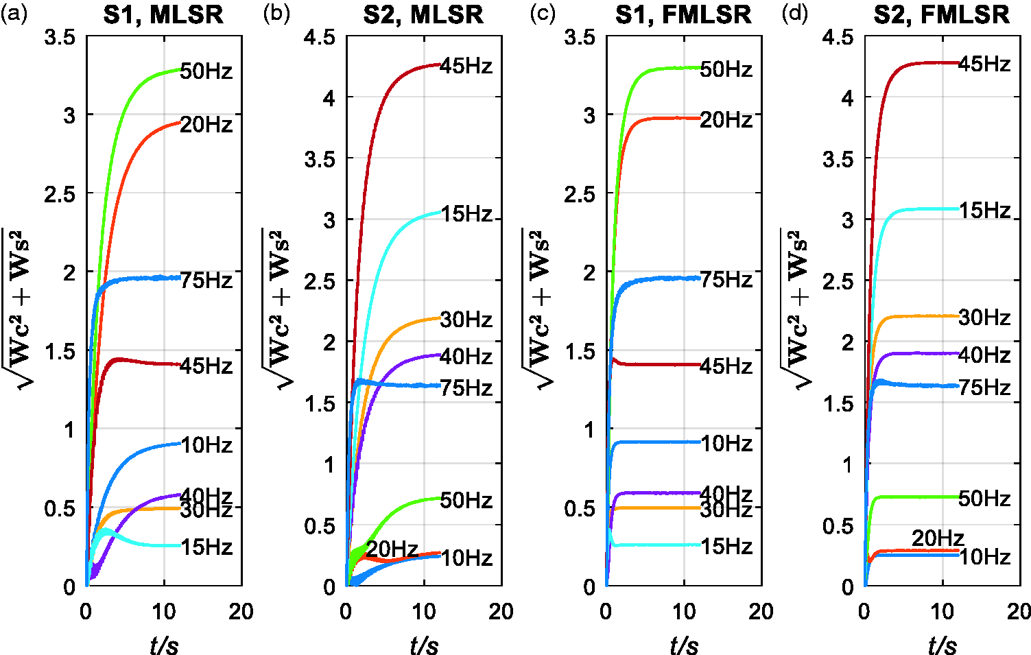
Convergence process of the controller coefficients at S1 and S2 of MLSR and FMLSR algorithm in Case A.

Case B: Two external sources, four local sources and four sensors

In case B, two external sources are placed at P1 and P2, and four local sources and four error sensors are placed at S1, S2, S3 and S4. The spectrums of external sources are the same as that in case A. The equalization parameters for S1, S2, S3 and S4 are defined to be the same, i.e. {1, 0, 0.4, 0, 1.5, 0, 0.4, 0}. Thus, the amplitudes of the target spectrums are {1 × 10⁻⁶ m, 0 m, 2 × 10⁻⁶ m, 0 m, 3 × 10⁻⁶ m, 0 m, 4 × 10⁻⁶ m, 0 m}. The simulation frequency is 2048 Hz, the sampling time is 30 s and the step-size is 1 × 10⁸.

According to Table 2, there are 43,504 multipliers and 9976 multipliers for MLSR and FMLSR, respectively, for Case A, in which the proposed FMLSR algorithm will reduce the computational complexity by 77% theoretically. The time consumption of the simulation in Case B has also been evaluated. In 50 independent trials, the average time consumption of MLSR and FMLSR was 101.88 ± 1.26 s and 27.18 ± 0.24 s, as shown in Figure 11. The operating environment and computing method are the same as those in Case A. Again, the simulation in Case B verified the superiority of the FMLSR in reducing the computational complexity.

Figure 11.

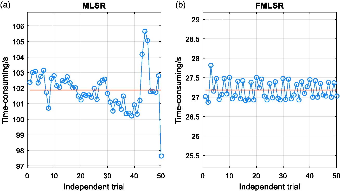
Time consumption of MLSR and FMLSR in Case B.

Figure 12(a) to (d) shows the real-error signal at S1, S2, S3 and S4, respectively. Figure 13(a) to (d) shows the pseudo-error signal at S1, S2, S3 and S4, respectively. It can be seen that all the pseudo-error signals approach to zero, and the real-error signals are first reduced and then increase and finally approach stable. Figure 14(a) to (d) shows the spectrum at S1, S2, S3 and S4, respectively, with control ON and OFF. It can be seen that all the spectra of all the target point have been modified and reach the predefined target.

Figure 12.

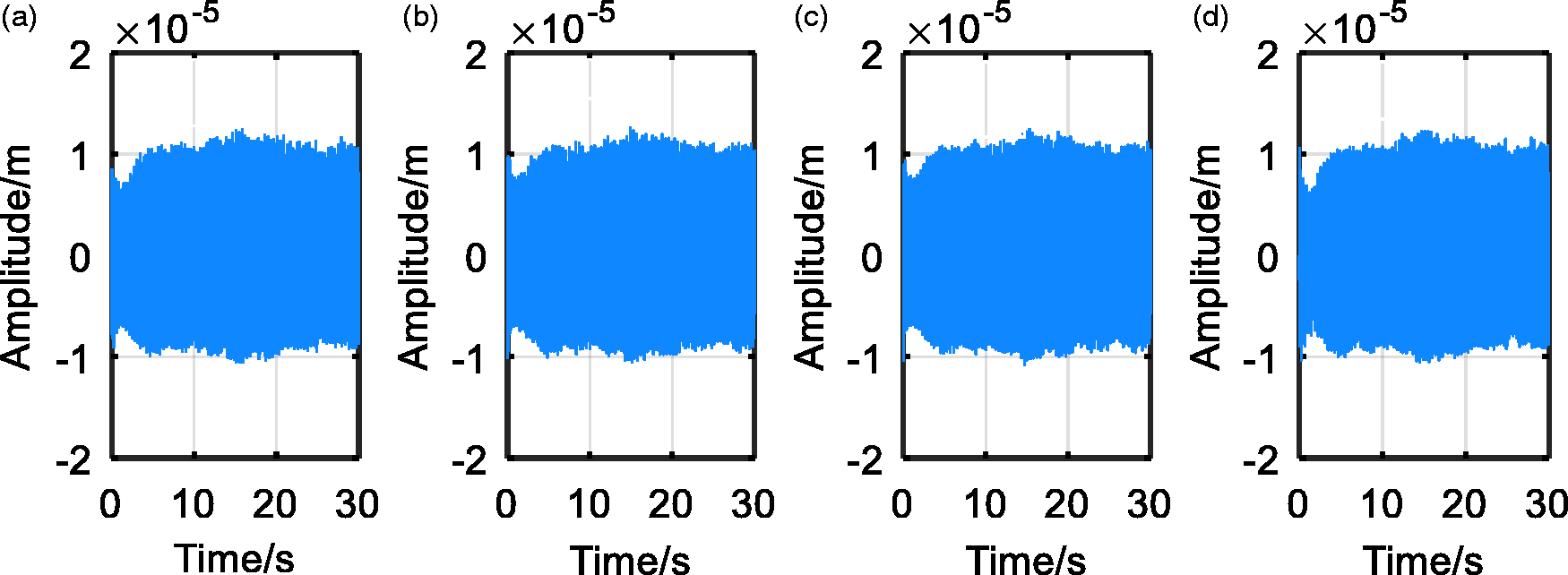
Real-error signal at S1 (a), S2 (b), S3 (c) and S4 (d).

Figure 13.

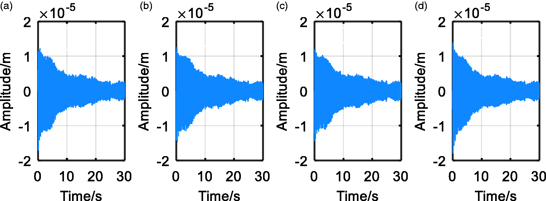
Pseudo-error signal at S1 (a), S2 (b), S3 (c) and S4 (d).

Figure 14.

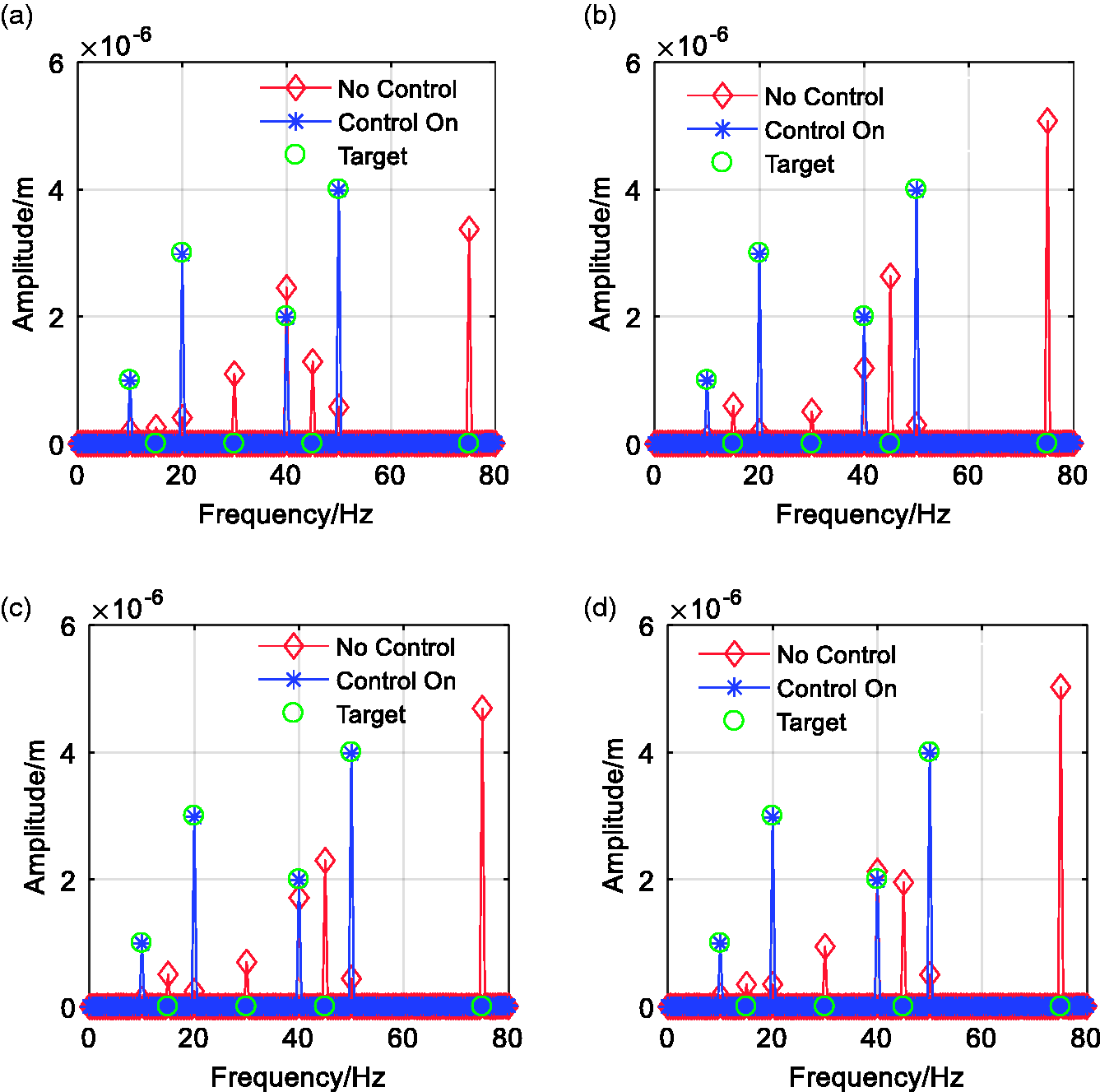
Multiline spectrums at S1 (a), S2 (b), S3 (c) and S4 (d) with control ON and OFF.

The convergence process of the two algorithms has also been compared using the controller coefficients in Case B, as shown in Figures 15 and 16. Figure 15(a) to (d) shows the coefficients of the MLSR algorithm at S1, S2, S3 and S4, respectively. Figure 16(a) to (d) shows the coefficients of the FMLSR algorithm at S1, S2, S3 and S4, respectively. It can be seen that just the same as Case A, the FMLSR has a more uniform (between components) convergence property than MLSR in Case B, which further verifies the superiority of FMLSR in improving the convergence property of the control system.

Figure 15.

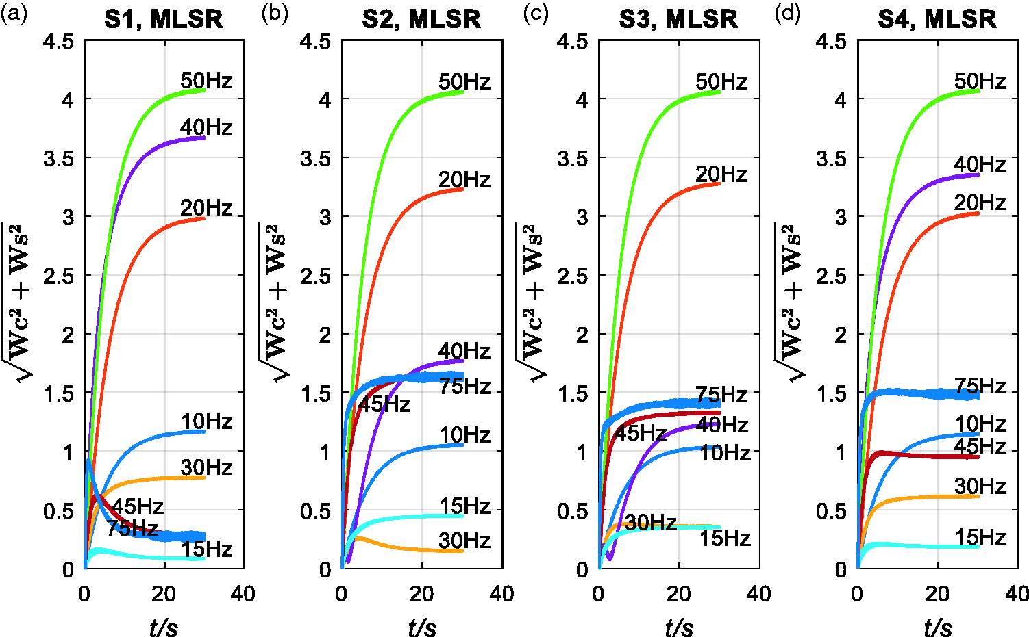
Convergence process of the controller coefficients at S1 and S2 of MLSR algorithm.

Figure 16.

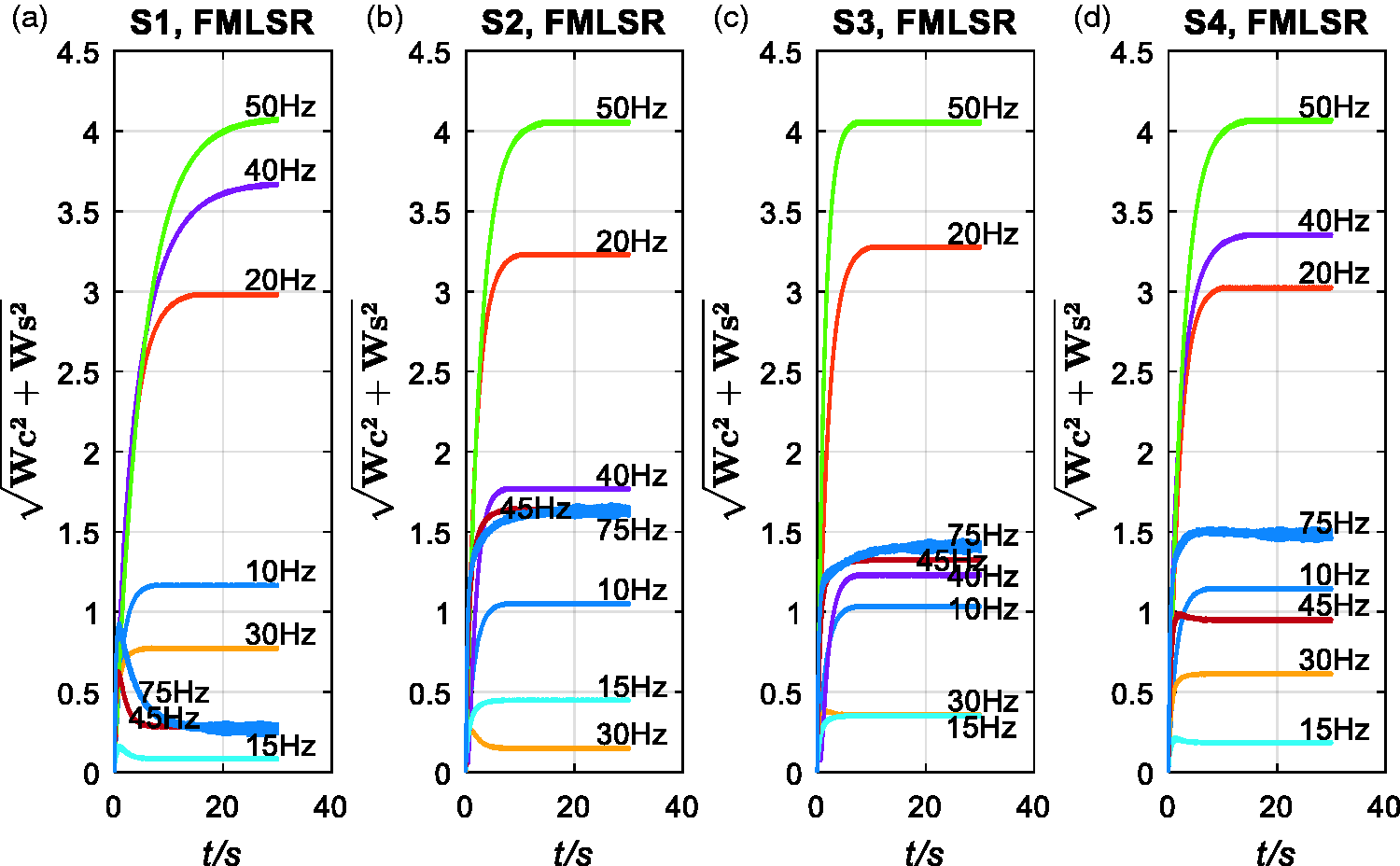
Convergence process of the controller coefficients at S1 and S2 of FMLSR algorithm.

Conclusion

In this study, we propose a fast algorithm for multiline spectral reshaping to overcome the problem of computational burden in the situation where the number of spectral lines, vibration sources and observation sensors is large. A phase schedule module has been introduced to generate reference signal directly instead of using filters. An equivalent system of the traditional MLSR algorithm has been constructed by introducing two extra canceling branches. Theoretical analysis shows that the proposed algorithm can reduce about 75% computational complexity compared to the traditional one. Numerical case studies on the FEMilS test-bed have been carried out to verify the effectiveness of the proposed algorithm. It shows that the proposed algorithm can perform an accurate residual vibration control with uniformed convergence speed and reduced computational complexity.