
Abstract
A piecewise hysteresis nonlinear dynamic model with nonlinear stiffness and damping is established for a system with alternating elastic constraints and hysteresis nonlinearity. First, the amplitude–frequency response equation of the system is solved by using the averaging method under periodic excitation. Two frequency regions with multiple solutions are then identified in the system, and the amplitude–frequency response characteristics under different system parameters are obtained. Thus, the influence law of different piecewise nonlinear factors on system stability is explored. Second, the bifurcation behavior of the system under different external disturbances is analyzed. Given the change of perturbation parameters, the system is found to be a complex dynamic system with alternating periodic, double periodic, and chaotic motions, and many other forms of movement. Moreover, lower buffer damping leads to the complex and unpredictable chaotic state of the system’s dynamic behavior.
Introduction
The piecewise problem of nonlinear systems widely exists in the field of natural science and engineering technology. The problem is mainly caused by the presence of clearances, dead-zone characteristics, dry friction, and switching among subsystems in the system structure, thereby leading to different nonlinear characteristics of the system in divergent motion stages.1–4 For instance, the piecewise problem in mechanical systems may lead to system clearances because of the existence of processing error, installation error, and subsequent wear. The system clearances will change the system movement behavior and will cause repeated shocks between the components and even lead to jumping, bifurcation, and chaos. Consequently, the dynamic behavior of the system becomes complex and unstable. 5 In another example, the characteristics of segment restraint, such as the friction buffer of heavy-duty train, the vibrating screen, and the grouped spring of the vibrating conveyor, have been applied in many systems to effectively improve their dynamic characteristics. 6
Three common analytic methods by He are available for nonlinear oscillators with discontinuities: the He’s frequency method, He’s homotopy perturbation, and He’s variational iteration. He’s7,8 frequency method is from the ancient Chinese mathematics method. Zhang 9 used He’s amplitude–frequency formulation to obtain a periodic solution of a nonlinear oscillator with discontinuity and demonstrated the simple solution procedure and the remarkable accuracy of the obtained solutions. He’s homotopy perturbation10,11 was developed by using the modified Lindstedt–Poincare method,12,13 wherein the solution and the coefficient of linear terms were expanded into a series of embedding parameters. Öziş and Yıldırım 14 compared two distinct adaptations of He’s homotopy perturbation method for determining the amplitude–frequency relation of a nonlinear oscillation with discontinuities. Zhu et al. 15 applied He’s homotopy perturbation method for discontinued problems in nanotechnology, and the comparison of the approximate solution with the exact one revealed that the method is effective. Beléndez et al. 16 modified He’s homotopy perturbation method to calculate the periodic solutions of a nonlinear oscillator with discontinuities, where the elastic force term is proportional to sgn(x). He and co-workers17,18 suggested He’s variational iteration method, a useful formulation for determining the approximate period of a nonlinear oscillator and overcoming the shortcoming of approximate solutions. Moreover, the examples illustrated the solution procedure. Rafei et al. 19 applied the variational iteration method of He to nonlinear oscillators with discontinuities and demonstrated that the variational iteration method is effective and convenient and does not require linearization or small perturbation. Tao 20 applied the variational method of He to obtain the amplitude–frequency relationship of some nonlinear oscillators with discontinuity. Recently, He 21 proposed the simplest approach to the cubic–quintic Duffing equation based on his previous research, thereby providing an extremely fast and relatively accurate estimation of the frequency of a nonlinear conservative oscillator.
For discontinuous damped nonlinear systems with external excitation forces, the averaging and incremental harmonic balance methods are widely used. Ji and Hansen 22 employed matching and modified averaging methods to construct an approximate solution for the super-harmonic resonance response of a periodically excited nonlinear oscillator with a piecewise nonlinear characteristic. The validity of the developed analysis was confirmed by comparing the approximate solutions with the results of the direct numerical integration of the original equation. Using an incremental harmonic balance method, Xu et al.23,24 solved a class of piecewise linear oscillators with asymmetric stiffness and viscous damping and compared the periodic solutions with different harmonic terms and the influence of system damping and external excitation on the amplitude–frequency characteristics of piecewise linear constrained systems.
Many studies have attempted to provide reasonable uses and avoid the adverse effects of the dynamic characteristics of the piecewise linear system in engineering design and application. Li and Chen 25 explored the circuit synthesis of a high-dimensional piecewise linear system with a piecewise linear element, proposed the synthesis method of a linear one-port circuit in piecewise linear chaotic circuit, and revealed the relationship between the system characteristic value and the working frequency of the circuit. Wu et al. 26 selected two different piecewise linear circuit systems as the subsystems of the switching system, implemented switching between the two subsystems with switch control, and analyzed the influence of nonsmooth factors and switching on system dynamics. Kalmár-Nagy et al. 27 simulated the aerodynamic force as a piecewise linear function of an effective dip angle for the aeroelastic system of the wing, established a piecewise linear aerodynamic model, determined the inherent bifurcation of the piecewise system, and observed the intermittent path of the system to chaos through numerical methods. Liu et al. 28 established a roll-over dynamics model of heavy-duty vehicles and examined the influence of tire and vehicle lateral stiffness in the model in terms of vehicle attitude response after piecewise linearization. Zhang et al.29,30 developed a piecewise linear dynamic system model of coupling with different time scales. They also surveyed its equilibrium and stability in different areas, the bifurcation behavior, and the corresponding critical conditions and the system trajectory through nonsmooth boundary surface of bifurcation analysis. Furthermore, they discussed the existence of different nonsmooth bifurcation conditions and behaviors. Du et al. 31 explored the phase sequence in one-dimensional piecewise linear discontinuous maps, analyzed the internal mechanism of disordered phase generation in multi-frequency chaotic systems, and proved that the phase sequence is sensitive to the density distribution of attractor trajectories.
With the rapid development of nonlinear theory, piecewise nonlinear problems, which are more general than piecewise linear problems, have attracted considerable attention in recent years. Yu et al.32,33 investigated complicated behaviors of the compound system with periodic switches between two nonlinear systems. Through local analysis, they found that critical conditions, such as fold and Hopf bifurcations, were derived to explore the bifurcations of the compound systems with different stable solutions in the two subsystems. Jin and Li 34 studied the stochastic resonance in a piecewise nonlinear system driven by a periodic signal and colored noises, which was described by multiplicative and additive colored noises with colored cross-correlation. They also derived the analytical expressions of the steady-state probability density and the signal-to-noise ratio. Li et al. 35 considered a one-degree-of-freedom (DOF) nonlinear moving belt system and derived the analytical research of a sliding region and the existence conditions of equilibrium. Kong et al. 36 examined the dynamic behaviors and the stability of the linear guide considering contact actions by a multi-term incremental harmonic balance method and formulated a generalized time-varying and piecewise nonlinear dynamic model of the linear guide to perform an accurate investigation of its dynamic behaviors and stability. Guo et al. 37 and Xi et al. 38 investigated the stochastic resonance in a piecewise nonlinear model driven by multiplicative non-Gaussian and additive white noise, and discussed the effect of noises, periodic signal, and system parameters on signal-to-noise ratio. Wang et al. 39 derived the relationship between contact deformation and force via Hertz contact theory and obtained piecewise nonlinear interaction forces. They also solved dynamic differential equations by using the Runge–Kutta integration method to investigate the dynamic behaviors of the dynamic system. Their results showed that the system exhibits softening nonlinear behavior in the primary resonance region under a small excitation force. Wang et al. 40 proposed an improved method to combine the incremental harmonic balance method with the equivalent piecewise linearization for solving the dynamics of complicated nonlinear stiffness systems. Moreover, they presented the Duffing oscillator to validate the proposed method. The results confirmed that the proposed method can analyze the dynamics of complicated nonlinear stiffness systems.
As the mathematical models of piecewise dynamic systems become increasingly complex, some models can only be analyzed with numerical methods. Therefore, some scholars began to study the numerical algorithms of piecewise dynamic systems. Yu 41 presented an efficient computational method for determining the vibrational responses of piecewise linear dynamical systems with multiple DOFs and an arbitrary number of gap-activated springs. A time-domain solution was obtained using the Bozzak–Newmark numerical integration scheme. The proposed method was successfully applied to a piecewise linear dynamical system with 1000 DOFs and 1000 gap-activated springs under harmonic excitations. Acary et al. 42 developed a method for the numerical analysis of one proposed extension, namely the Aizerman–Pyatnitskii extension, by reformulating piecewise-linear models as a mixed complementarity system. This approach allowed for the application of methods developed for this class of nonsmooth dynamical systems. He et al. 43 proposed the computation of dynamic responses of periodic piecewise linear systems with multiple gap-activated springs based on the parametric variational principle. This method indicated numerous identical and zero elements in the matrix exponents of a periodic structure and saved computation load and computer storage by avoiding the repeated calculations and storage of these elements.
Overall, the studies on piecewise dynamic systems mainly consider such aspects as piecewise linearity, symmetric piecewise nonlinearity, subsystem switching, and scale coupling in different frequency domains. However, no research has been conducted on the dynamic behavior of the hysteretic nonlinear system with multiple piecewise points. Thus, a class of piecewise nonlinear dynamic model with nonlinear stiffness and damping is established for a dynamic system with clearances, stroke elastic constraint, and viscoelastic buffer. On the basis of the model, several works are conducted:
The amplitude–frequency response relation of the system under periodic excitation is solved. The periodic response characteristics of the system under different constraints are discussed. The bifurcation behavior of the system under different external disturbances is analyzed.
Dynamical model
Theoretical model
In engineering applications, the piecewise nonlinear problem can be expressed as the clearance between the buffer and the isolated object and the elastic collision when the buffer reaches its maximum stroke. The buffer, which is formed by metal rubber, elastic cement, magnetorheological fluid, and other materials, is widely available in engineering vibration systems. Given this type of buffer, the system will demonstrate hysteresis nonlinear characteristics due to the existence of dry friction, internal damping, and other factors.
Taking the longitudinal dynamic system of a heavy-haul railway freight car as an example, the coupler buffer of such car comprises a steel spring, dry friction parts, and elastic cement, and the force from the buffer to the car body shows hysteresis nonlinearity. Moreover, the system will have multiple segmentation points due to the effect of coupler clearance and buffer stroke. Therefore, the longitudinal vibration system between the heavy-haul railway freight car body and the coupler buffer can be simplified into a piecewise nonlinear model as shown in Figure 1.
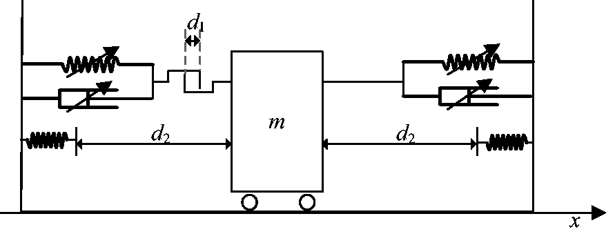
Piecewise hysteresis nonlinear system.
In Figure 1, m is the quality of the heavy-haul railway carriage, x is the vibration displacement of the carriage, d1 is the coupling clearance, and d2 is the maximum stroke of the buffer. The following three conditions are discussed:
When carriage displacement x is smaller than the coupling clearance d1 (i.e. When When carriage displacement x approaches the maximum stroke of buffer (i.e.
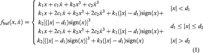
A mechanical model of piecewise nonlinear buffer is proposed as shown in equation (1)


Dividing both sides of equation (3) by m, the equation can be simplified as a dimensionless form expressed by equation (4)

With the use of the model, the response of this piecewise hysteresis nonlinear system under periodic excitation can be analyzed, and the influence of buffer clearance and parameters on system dynamic behavior can be studied.
Solution of system response under excitation
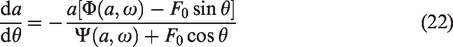
According to the characteristics of piecewise nonlinear constraints, the average method is used to solve the system in equation (4). Let be


Subsequently, let


Making equation (8) for differential time t

Substituting equation (9) with equation (11) generates the following

Equation (13) is obtained as follows

Expressing equation (9) for differential time t

Substituting equations (8) and (14) with equation (6) generates the following

Equation (15) is simplified to equation (16)

From equations (13) and (16), the differential equations of


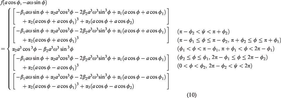
Average value in one period of


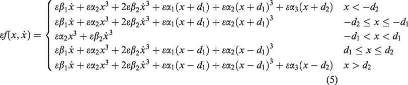
In the following conditions, when
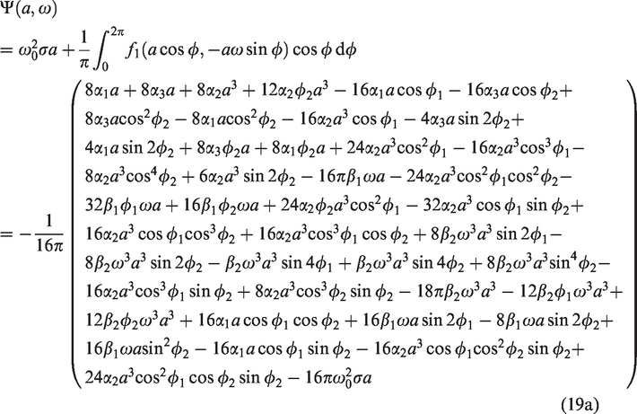
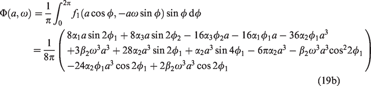
When
When


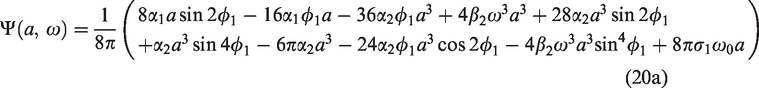
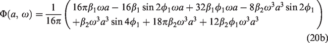
From equation (18), the first-order differential equation for the autonomous form is as follows
After obtaining the value of excitation

Periodic response characteristics of piecewise hysteretic nonlinear systems
Verification
Equation (2) is solved using the Runge–Kutta numerical method to verify the accuracy of the approximate analytical solution of the main resonance of the system calculated by the average method. The following system parameter values are assumed:
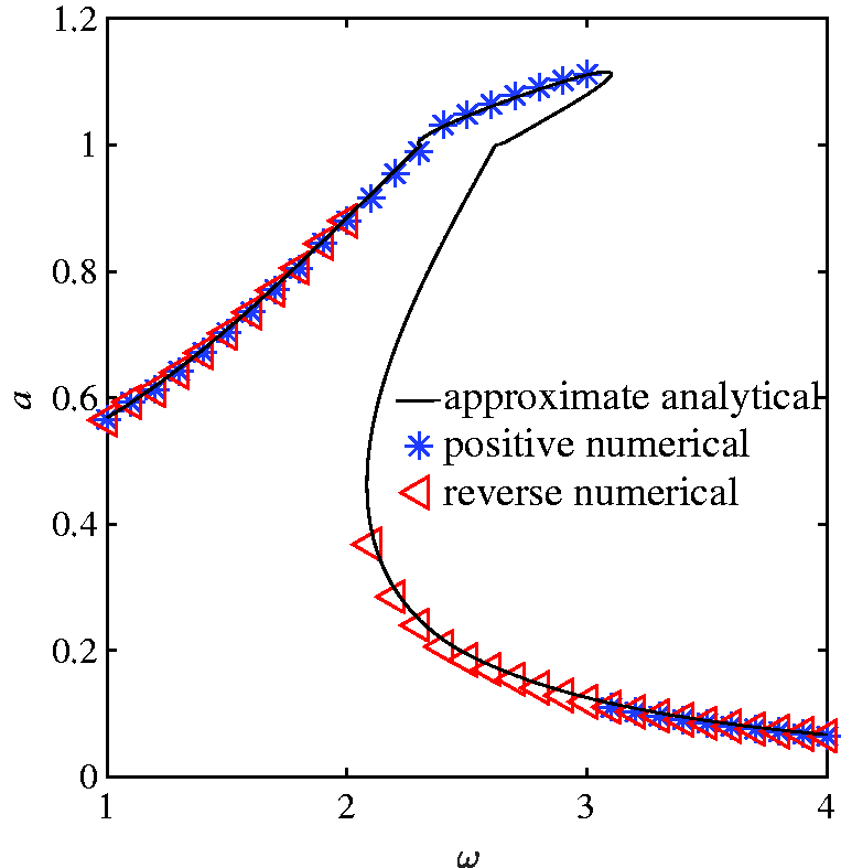
Comparison of approximate analytical and numerical solutions.
Amplitude–frequency response characteristics
The amplitude–frequency response curve is shown in Figure 3. The figure also indicates the emergence of the hysteresis phenomenon and four jumps for the system amplitude when the external excitation frequency slowly changes.
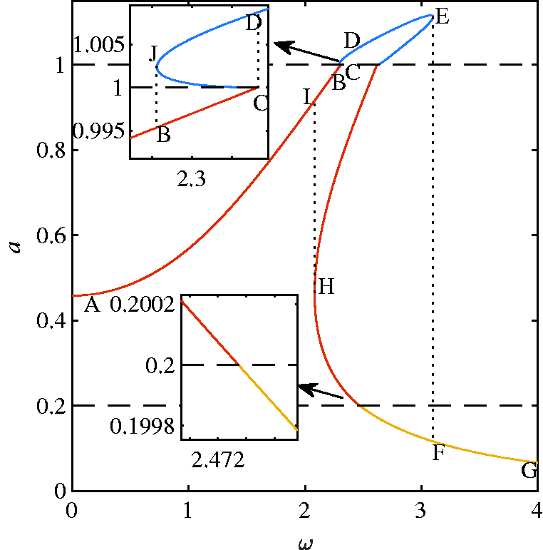
Amplitude–frequency response curve and local enlarged view of the system.
When the external excitation frequency increases from 0 to another value, the system amplitude varies along the curve AIB to point C. The frequency continues to increase, and the amplitude jumps from points C to D. Afterward, the amplitude continues to change along curve DE to point E. At this moment, if the frequency continues to increase, then the amplitude jumps from points E to F and varies along curve FG.
By contrast, when the external excitation frequency decreases from point G, the system amplitude varies along curve GF to point H and jumps to point I. Thereafter, the amplitude will change along curve IA.
When the steady-state of the system remains in a state corresponding to curve EDJ, the system amplitude varies along curve EDJ and then jumps from point J to point B and changes along curve BIA if the external excitation frequency gradually decreases. According to the JC and HE segments in the amplitude–frequency response curve, the system vibration is unstable.
According to the local magnification part in Figure 3, under the existing parameters, the amplitude–frequency curve is a smooth transition when the critical position of piecewise nonlinear constraint reaches d1. However, if the critical position comes to d2, then the amplitude–frequency curve becomes an evident nonsmooth deflection, thereby leading to a jump phenomenon of the system and presents a smooth characteristic after passing the critical position.
If one of the parameters changes, such as the piecewise nonlinear constraints, then the piecewise point or the external excitation coefficient and the relation curve of system amplitude and external excitation frequency are compared as shown in Figures 4 to 9. The system’s nonlinear characteristics, which are subjected to piecewise nonlinear elastic and damping constraints, are analyzed. In addition, the variation law of the stability of piecewise hysteresis nonlinear constrained system affected by various parameters under variable excitation is discussed.
Figure 4 shows that under the influence of piecewise hysteresis nonlinear constraints, the curvature size of the amplitude–frequency curve increases with the growth of linear stiffness
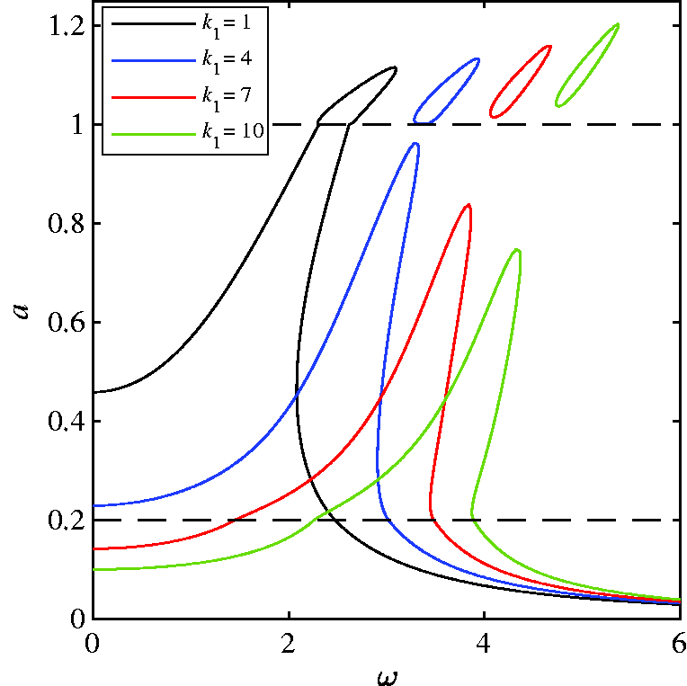
Amplitude–frequency response curve as linear stiffness k1 changes.
Figure 5 shows that when the nonlinear stiffness coefficient is small, the curve is less inclined if the amplitude is less than d2. However, the curve turns to a significant deflection if the amplitude becomes larger than d2, which means that the linear stiffness k2 at this time will result in strong nonlinearity and an unstable region for the system.
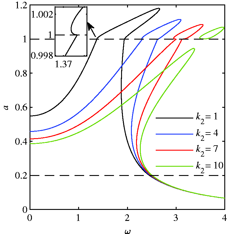
Amplitude–frequency response curve as nonlinear stiffness k2 changes.
When the nonlinear stiffness coefficient increases, the amplitude–frequency response curve becomes considerably curved. The local magnification part in Figure 5 shows a nonsmooth deflection in the curve at the position of d2 when the nonlinear stiffness coefficient is small. Nonlinear stiffness coefficient k2 continues to grow, and the refraction degree of the curve increases. Thus, an independent ring will appear in the curve, and the unstable frequency region will be widened.
Figure 6 shows that the system amplitude does not vary monotonically with the linear damping c1 due to the variation of piecewise nonlinear constraints. When the system excitation frequency increases, the amplitude will decrease with the increase of c1. However, if the external excitation frequency continues to increase to some value with a system amplitude larger than d2, then a certain frequency range will appear. At this range, large linear damping c1 leads to a large amplitude. Moreover, with the increase of c1, the curvature size increases, and an independent ring appears at the position of d2.
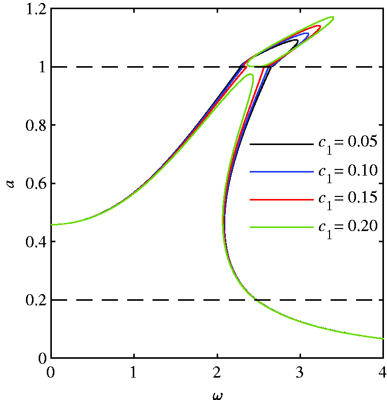
Amplitude–frequency response curve as linear damping c1 changes.
Similarly, the system amplitude does not vary monotonically with the linear damping c2 (Figure 7). When the system excitation frequency increases, the amplitude will decrease with the increase of c2.
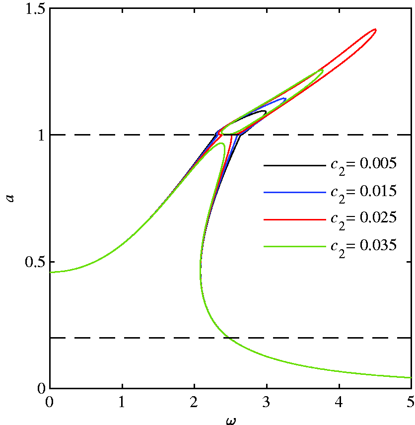
Amplitude–frequency response curve as nonlinear damping c2 changes.
If the external excitation frequency increases to a certain range, then the system amplitude will first increase with c2 in this range (e.g. the system amplitude of c2 = 0.025 is larger than that of c2 < 0.025 in Figure 7). If c2 continues to increase, then the system amplitude will decrease, and an independent ring will appear (e.g. the system amplitude of c2 = 0.035 is smaller than that of c2 = 0.025).
Figure 8 shows that the system amplitude increases with the external excitation coefficient
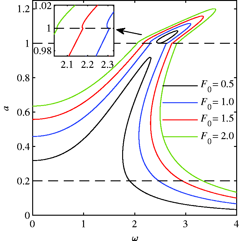
Amplitude frequency response curve as external excitation force F0 changes.
Figure 9 shows that with the increase in d1, the frequency at which the system jumps decreases, and the nonlinear refraction at d2 increases. Furthermore, the system amplitude increases with d1 for the left branch of the curve, and the opposite is true for the right branch.
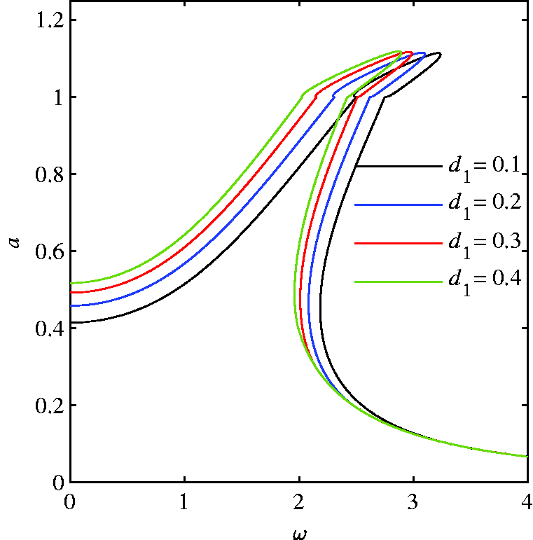
Amplitude–frequency response curve as piecewise point d1 changes.
Bifurcation response characteristics
By taking clearance d1 as the bifurcation parameter, equation (2) is solved using the Runge–Kutta numerical method. The system parameter values are as follows:
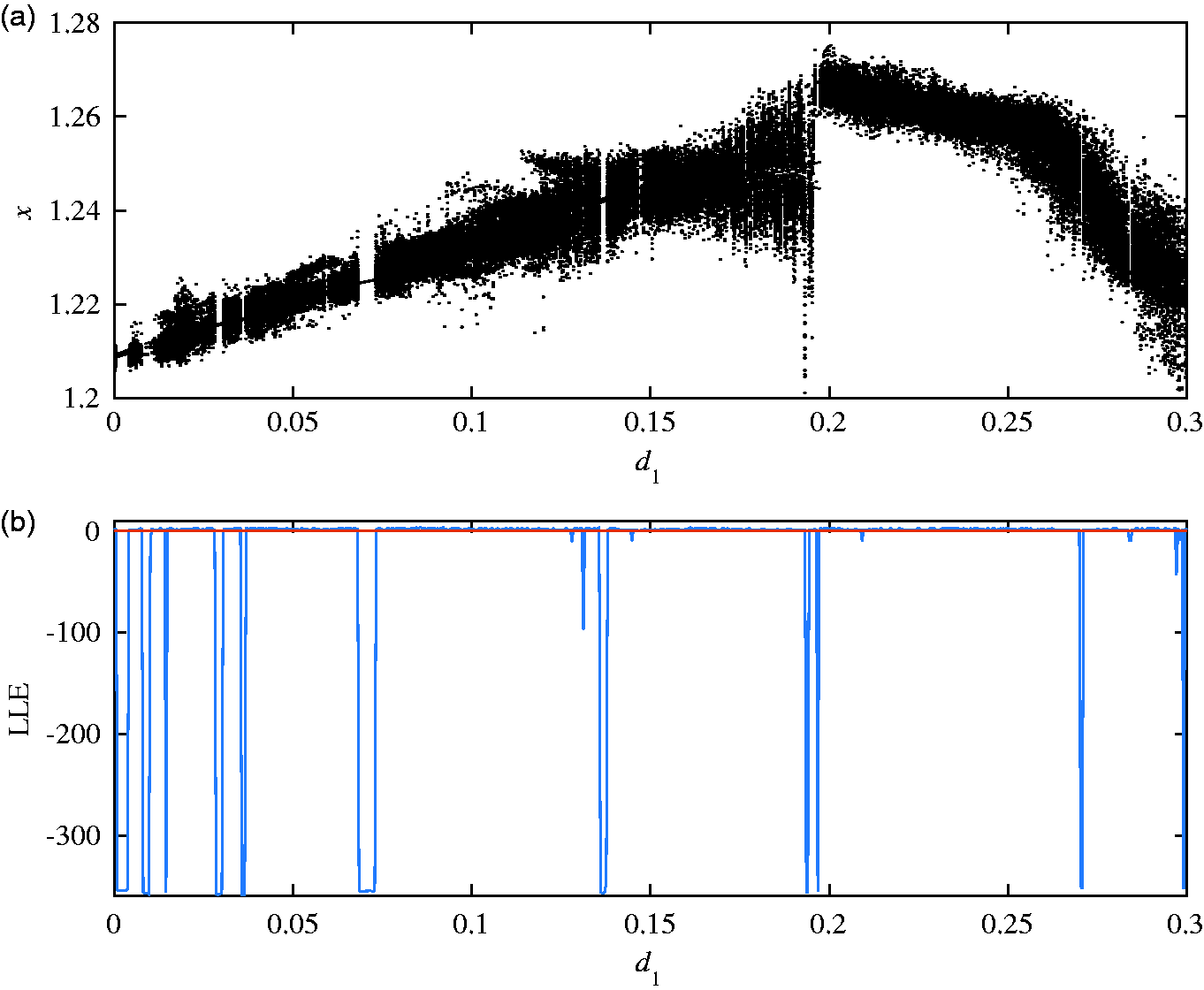
The influence of the system clearance on system dynamic behavior is studied. In addition, the bifurcation diagram of the system under clearance and its corresponding largest Lyapunov exponent curve are analyzed, as shown in Figure 10. The piecewise nonlinear constraint system has a complex dynamic behavior with the change of clearance d1 (Figure 10). Figures 11 to 13 show that the phase plane characteristics and Poincaré cross-section of the system were investigated because clearance value d1 is different.
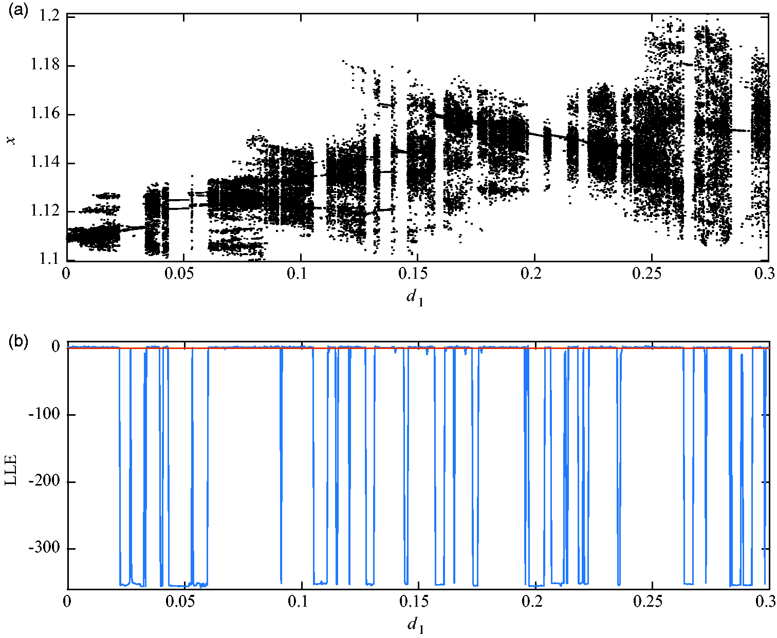
When c1 = 0.7, (a) is the bifurcation diagram of the system and (b) is the largest Lyapunov exponent curve of the system. LLE: largest Lyapunov exponent.
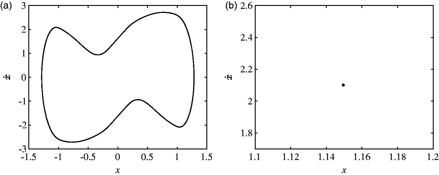
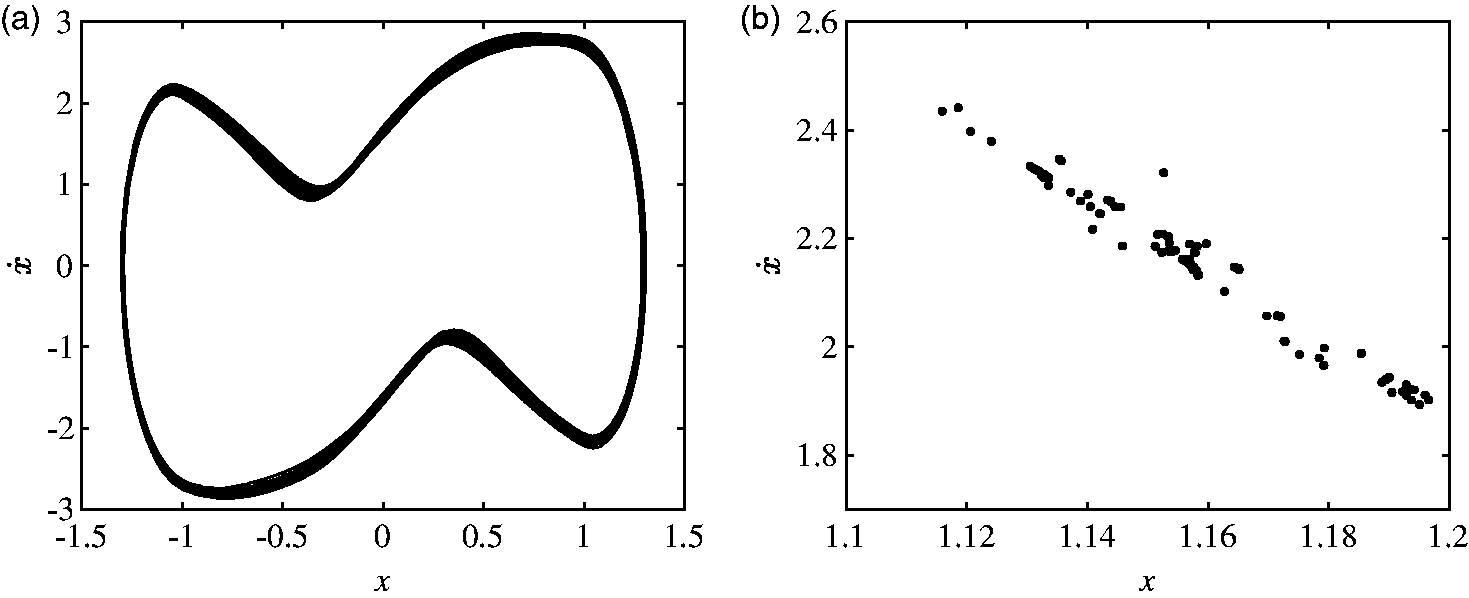
When c1 = 0.7, d1 = 0.219, (a) shows the phase diagrams of the system and (b) presents the Poincaré sections of the system.
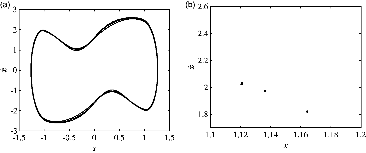
When c1 = 0.7, d1 = 0.135, (a) shows the phase diagrams of the system and (b) illustrates the Poincaré sections of the system.
When c1 = 0.7, d1 = 0.27, (a) shows the phase diagrams of the system and (b) presents the Poincaré sections of the system.
When d1 = 0.219, the system is a periodic motion. When d1 = 0.135, the system is a periodic four motion, and two of the phase loci are close to each other. When d1 = 0.27, several overlapping points are randomly distributed in the Poincaré cross-section of the system, an outcome which indicates that the system is in chaotic motion.
Owing to the change of clearance d1, the system will alternate between periodic, double periodic, and chaotic motions. By properly adjusting the system clearance, the system can be in a predictable periodic motion state.
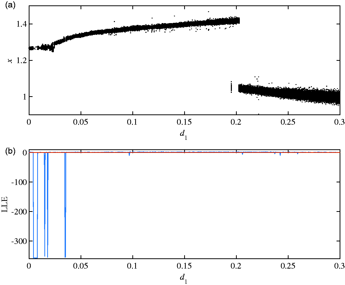
The influence of the buffer’s linear damping on the system stability is studied by comparing the bifurcation characteristics of the system with the clearance when the linear damping changes. Figures 10, 14, and 15 show that with the decrease of the buffer’s linear damping, the clearance interval with LLE less than 0 will decrease, whereas those that remain in the chaotic region will increase. Thus, the decrease in the buffer’s linear damping will lead to a complex and unpredictable chaotic state of the system’s dynamic behavior in a wide range and will gradually destroy the stability of the system.
When c1 = 0.4, (a) shows the bifurcation diagram of the system and (b) depicts the largest Lyapunov exponent curve of the system. LLE: largest Lyapunov exponent.
When c1 = 0.05, (a) shows the bifurcation diagram of the system and (b) depicts the largest Lyapunov exponent curve of the system. LLE: largest Lyapunov exponent.
Conclusion
Piecewise hysteresis nonlinear dynamic models with nonlinear stiffness and damping are proposed for systems with clearances, travel elastic constraints, and hysteresis nonlinearity. The periodic response of the piecewise hysteresis nonlinear system is then solved using the average method, and the amplitude–frequency response characteristics of the system are obtained. Two frequency regions with multiple solutions are also found in the system.
Through analysis, the following conclusions are drawn.
First, the analysis of the influence law of different parameters on the system response revealed that increasing linear and nonlinear stiffness, linear and nonlinear damping, and excitation force will widen the unstable frequency region of the system.
Second, the influence of linear and nonlinear damping on the system amplitude is not monotonic. A certain frequency interval indicates that a large linear and nonlinear damping leads to large system amplitude. In other frequencies, the opposite is true.
Finally, the bifurcation response characteristics of the system are numerically studied, and the system is found to alternate between periodic, double periodic, and chaotic motions with the change of the clearance. Moreover, the reduction of linear damping will put the dynamic behavior of the system in a complex and unpredictable chaotic state in a wide range.
Footnotes
Declaration of conflicting interests
The author(s) declared no potential conflicts of interest with respect to the research, authorship, and/or publication of this article.
Funding
The author(s) disclosed receipt of the following financial support for the research, authorship, and/or publication of this article: This work was supported by the Major Program of the National Natural Science Foundation of China (No. 11790282), the National Natural Science Foundation of China (No. 11702179, 11802183), the Young Top-Notch Talents Program of Higher School in Hebei Province (No. BJ2019035), and the Preferred Hebei Postdoctoral Research (No. B2019003017).