Sage Journals: Discover world-class research

Abstract

Technology that measures bridge responses when a vehicle is crossing over it for structural health monitoring has been under development for approximately a decade. Most of the proposed methods are based on identification of the dynamic characteristics of a bridge such as the natural frequency, the mode shapes, and the damping. Specifically, many time–frequency domain approaches have been used to extract complex spectrum signatures from the complicated vibrations of a bridge due to the interactions of a vehicle with the bridge, which usually involves nonlinear, nonstationary, stochastic, and impact vibrations. In this paper, a method known as complete ensemble empirical mode decomposition with adaptive noise is applied for the first time to analyze the acceleration response of a bridge to a moving vehicle, and the purpose is to extract the spectrum signature of the vehicle–bridge response for structural health monitoring. The time–frequency Hilbert-Huang transform (HHT) spectrum of the decomposed mode from complete ensemble empirical mode decomposition with adaptive noise is presented. The results are well-correlated with finite element analysis. The advantages of the complete ensemble empirical mode decomposition with adaptive noise method are demonstrated in comparing the data from conventional methods, including power spectra, spectrograms, scalograms, and empirical mode decomposition.

Keywords

Complete ensemble empirical mode decomposition with adaptive noise vehicle–bridge interactions bridge structural dynamic structural health monitoring

Introduction

The use of vehicle–bridge interaction data for structural health monitoring (SHM) has received considerable interest in the last decade.^1–6 Compared with traditional bridge health monitoring, a vehicle–bridge interaction data-based approach allows target bridges to be monitored or assessed under operating conditions. In principle, the vehicle–bridge interaction and response have complicated nonlinear features, nonstationary features, and stochastic features. As such, varied spectrum analysis methods have been used to extract the vehicle–bridge response signature. Time–frequency characteristics for vehicle–bridge responses are widely analyzed using various methods including the time–frequency spectrum, the wavelet transform, and the Hilbert–Huang transform.

Time–frequency analysis can effectively reveal the constituent frequency components of nonstationary signals and their time-varying features, as well as transient events such as impulses.^7–9 To date, various time–frequency analysis methods have been proposed. However, the inherent drawbacks of these time–frequency analysis methods limit their effectiveness for analyzing complex vibration signals. For instance, linear transforms, such as the short time Fourier transform and the wavelet transform, are subject to the Heisenberg uncertainty principle, i.e. the best time localization and highest frequency resolution cannot be achieved simultaneously.¹⁰ One can only be enhanced at the expense of the other, hence the time–frequency resolution of linear transforms is limited. In addition, the basis in either the Fourier or the wavelet transform is fixed. Therefore, these transforms lack adaptability for simultaneously matching the complicated components inherent in complex vibration signals, such as the fundamental frequency and its harmonics, combined harmonics, chaos, system induced impulses, and other transient vibrations. As a typical type of bilinear time–frequency representation, the Wigner–Ville distribution has the best time–frequency resolution, but it has inevitable cross-term interference for multiple component signals. Such cross-term interference complicates the interpretation of the signal features in the time–frequency domain and makes this method unsuitable for analyzing complex vibration signals. Various modified bilinear time–frequency distributions including the Cohen and the affine class distributions may suppress the negative effects of cross-terms, but they will compromise time–frequency resolution and auto-term integrity.^11,12 In comparison with the Cohen and the affine class distributions of fixed kernel functions, the adaptive optimal kernel method can suppress the cross-terms more effectively with better time–frequency resolution.¹³ Wigner–Ville and Choi–Williams distributions introduce many distortions due to interference terms and negative components. They also require an extended computational time. Spectrogram better preserves the energy distribution (compared to the wavelet transform), but it has issues with time–frequency resolution and gives rather rough estimates. Wavelet transforms and scalograms provide good results, but they add artifact to frequencies close to zero or close to the edges. Additionally, they distort the energy distribution: high frequencies have less power than the lower ones.^7,13

The well-known Hilbert–Huang transform has fine time–frequency resolution and is free of cross-term interference, but it essentially relies on the empirical mode decomposition (EMD) using spline interpolation.⁸ It is susceptible to singularities in signals, and it may produce pseudo intrinsic mode functions (IMF), thus masking or interfering with the time–frequency structure of the true signal components. Oscillations of different amplitudes are found in a mode or similar oscillations are encountered in different modes. To avoid this problem, Wu and Huang¹⁴ proposed ensemble EMD (EEMD), which is a method based on the EMD algorithm. The proposed method follows the study of the statistical characteristics of white noise, involves noise-assisted analysis, and adds white noise of a uniform frequency distribution to EMD to avoid mode mixing. However, EEMD brings new problems, as the added white noise is not fully eliminated, and different modes may be produced by the interaction between the signal and the noise.^15,16 To resolve these issues, complementary EEMD (CEEMD) was introduced by Yeh et al.¹⁷ After adding positive and negative white noise to the signal, the signal is subsequently decomposed by EEMD. The final IMFs can be obtained by averaging the IMFs produced in the EEMD decomposition for signals with added positive and negative white noise.¹⁸ Nevertheless, this method has a high computational cost and does not resolve the additional modes. To remedy the issues of previous CEEMD methods, complete EEMD with adaptive noise (CEEMDAN) was proposed by Torres et al.¹⁹ This method in principle eliminates the problem of mixing modes of dramatically different periods into a single component, which may occur in previous EMD, EEMD, and CEEMD methods.

Unlike its predecessors, EMD, EEMD, and CEEMD, CEEMDAN resolves the mode mixing problem and provides better spectral separation for the modes. This method reduces computational load and overcomes additional modes. This method has been applied in various communities, and all applications have verified the advantages of this method.^19–27 The new CEEMDAN algorithm has the advantage of achieving a complete decomposition with no reconstruction error.

EMD and EEMD methods have been widely applied for bridge health monitoring.^28–40 In this paper, CEEMDAN is applied for the first time to analyze the acceleration response of a bridge to a moving vehicle. To demonstrate the effectiveness of the CEEMDAN-based method, we use CEEMDAN to decompose a transient spectrum into serial components. We can use these components to quantify the system properties and improve the performance of spectral discrimination for vehicle–bridge responses, which will demonstrate that this is an effective feature extraction scheme for SHM. The overall performance of CEEMDAN is also compared to state-of-the-art methods including spectrograms, scalograms, and EMD.

Techniques from the field of SHM have emerged as important tools to inspect and maintain bridge system structures. The natural mode monitoring-based approach has been widely investigated and used for SHM. However, vibrations of real bridges under passing vehicle excitation exhibit time-varying, nonlinear, and stochastic features. Conventional spectrum analysis methods such as spectrograms and scalograms have low resolution for this type of complex problem due to cross-term interference, and thus cannot effectively reveal the nonstationary constituent frequency components and their time-varying features such as transient mode mixing. The EMD-based Hilbert–Huang transform has fine time–frequency resolution and is free of cross-term interference. As the most advanced EMD method, CEEMDAN substantially improves EMD. In the present paper, the results show that there is more than 10% difference between the estimated specific transient frequencies from EMD and CEEMDAN. This research offers some insights for bridge agencies that can make use of the Hilbert spectrum of CEEMDAN as a more reliable index than conventional spectra or natural modes for system deterioration estimation and informed-decision making regarding maintenance and repair of bridge systems.

Bridge description

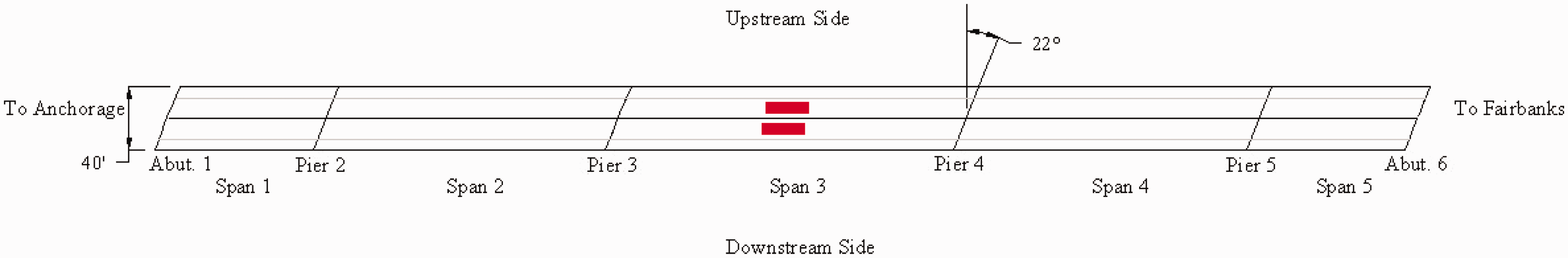
The Chulitna River Bridge is a steel girder composite bridge (Figure 1). It was built in 1970 on a 22° skew. The bridge is 790 ft long with five spans of 100, 185, 220, 185, and 100 ft. The superstructure was 34 ft wide by 6¾ in. thick cast-in-place concrete deck supported by two exterior continuous longitudinal variable depth girders and three interior stringers. The girder stringers are spaced at 7 ft on the center. The interior stringers are supported by a cross frame that is carried by the exterior girders. The cross frame was detailed to transfer dead loads and traffic loads to the exterior girders. Interior stringers were W21×44, and the exterior girders had a variable depth web that varied from 84 in. deep in the first and fifth spans to 108 in. deep in the third spans. Figure 2 shows the pier and span locations. At Piers 2 and 4, the exterior girder web has a haunch depth of 148 in. At Pier 3, the exterior girder web has a haunch depth of 168 in. In 1993, the bridge deck was widened from a 34 ft cast-in-place concrete deck to a 42 ft 2 in. concrete deck made of precast concrete deck panels. The increased load was accounted for by strengthening the variable depth exterior girders and converting the W21x44 interior stringers to an interior truss girder; the W21x44 became the upper chord of the truss.

Figure 1.

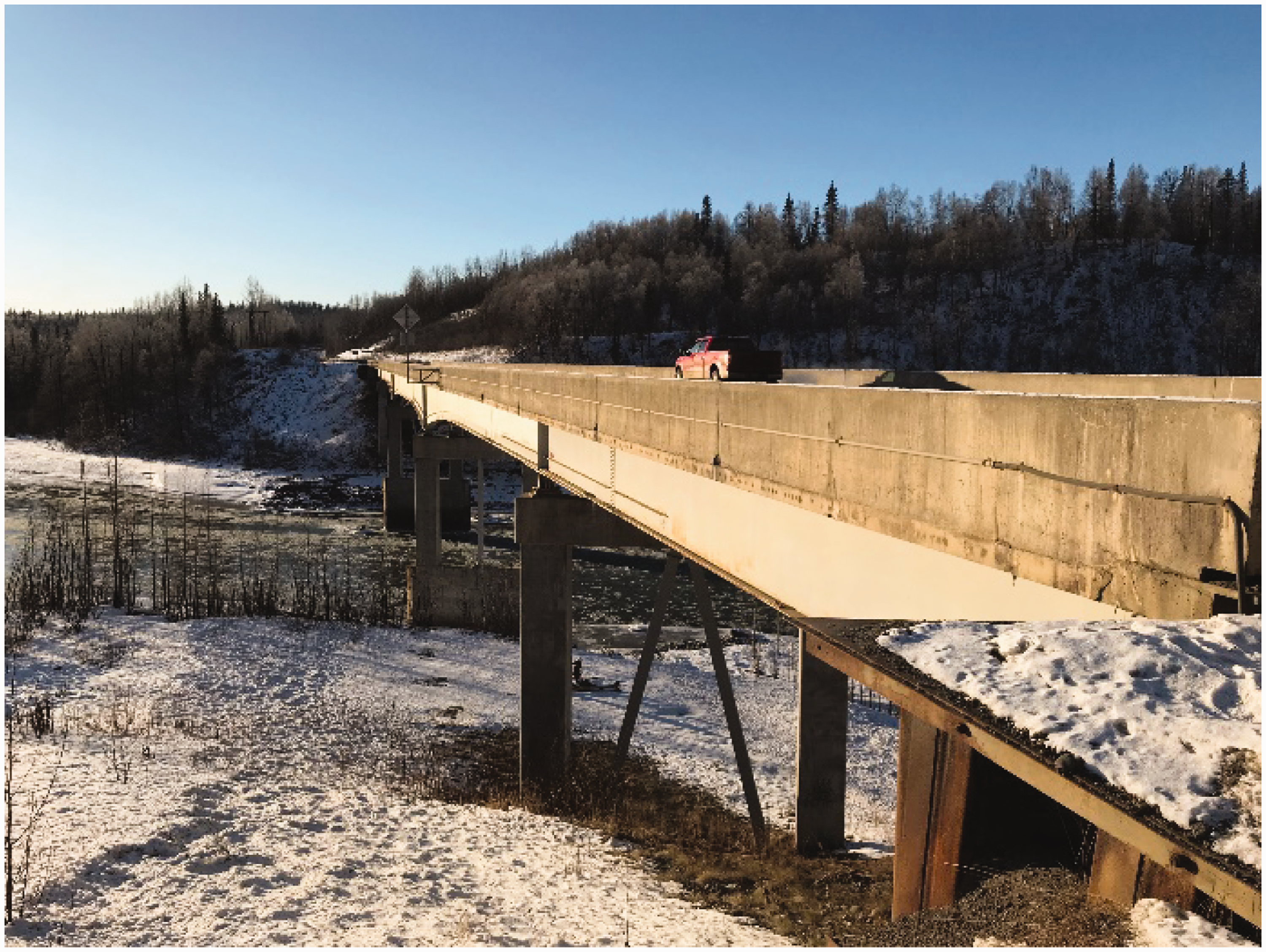
Chulitna River Bridge.

Figure 2.

Two trucks side by side.

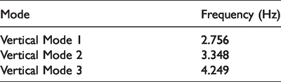
A finite element model of the bridge was developed using the commercial software SAP2000. The bridge trusses were modeled using frame elements, and the deck, stringers, and girders were simulated using shell elements. Detailed modeling and analysis results are included in Xiao et al.⁴¹ The natural frequencies of the first three vertical bending modes are listed in Table 1.

Table 1.

Finite element model results.

Mode	Frequency (Hz)
Vertical Mode 1	2.756
Vertical Mode 2	3.348
Vertical Mode 3	4.249

Testing of the bridge under passing vehicle

A dynamic load test was conducted on the bridge using two trucks. The trucks were loaded with sand and then the gross weights were measured, which were 82,100 and 80,250 lb. The two trucks were side by side (Figure 2) heading north (to Fairbanks) at 45 mile/h. Figure 3 shows the test trucks. A fiber optic bridge health monitoring system recorded the bridge’s dynamic response.

Figure 3.

Load test trucks.

A fiber optic SHM system was installed on this bridge to monitor the bridge’s real-time behavior.⁴² The system consisted of five parts: an optical sensing interrogator, a channel multiplexer, optical sensors, a local computer, and a remote computer. The optical sensing interrogator and the local computer are in the control panel at Princess Hotel, which is 1.5 mile away from the bridge site (Figure 4).

Figure 4.

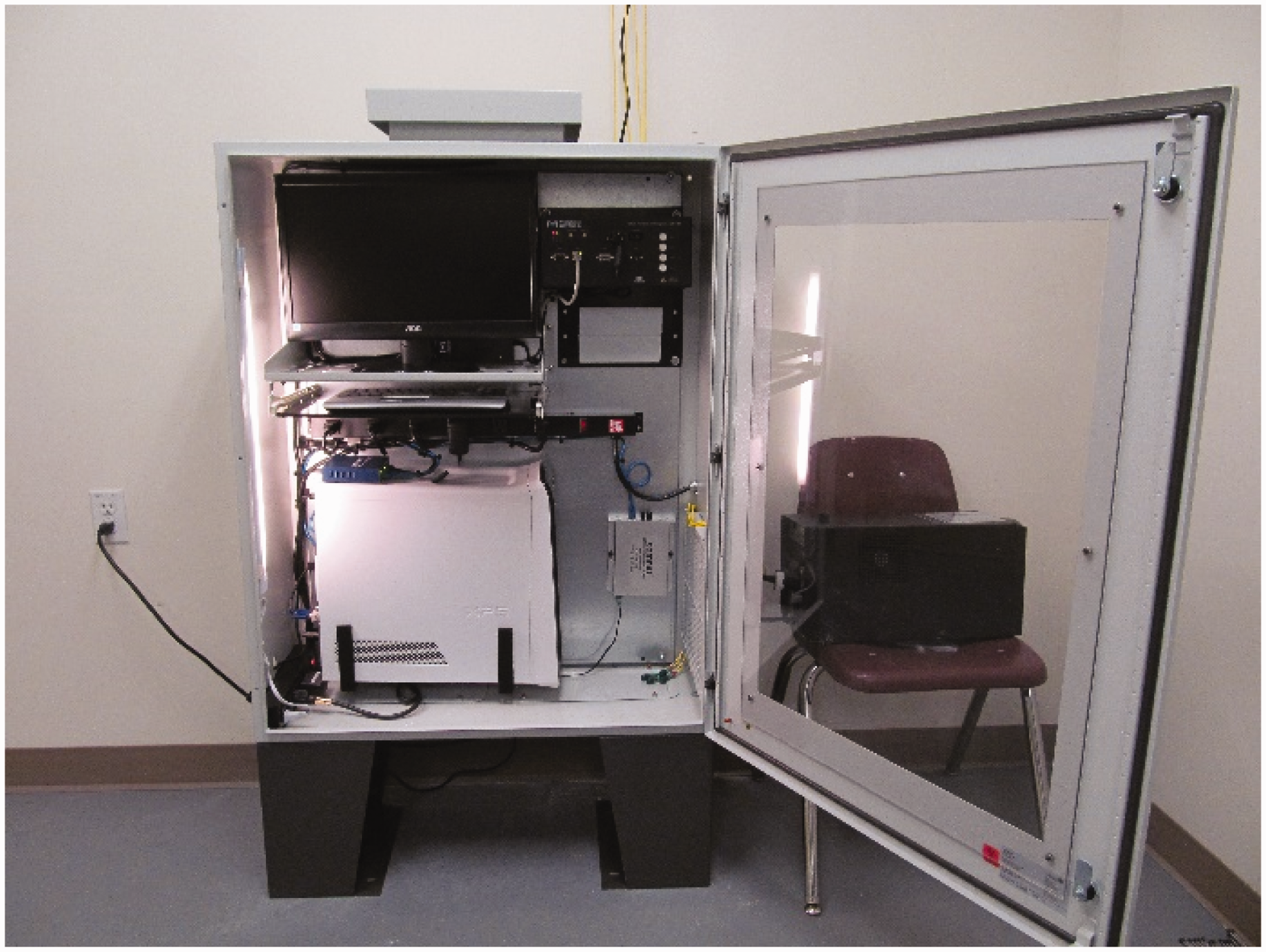
Local computer and interrogator.

The fiber optic accelerometer is as accurate and stable as conventional accelerometers. The advantages of fiber optic technology include long-term stability, nonconductive properties, and convenience. The light signal transmits a very long distance with very low signal transmission loss. The fiber optic sensor is made up of glass and a protective cover, and it is free from corrosion, giving it long-term stability. Fiber optic sensors have the advantage that they are nonconductive, which keeps them free from electromagnetic and radio frequency interference. Fiber optic sensors are practical to use in city areas that have serious signal interference. Additionally, fiber optic sensors and cables are very small and light, making it possible to permanently incorporate them into structures. On the other hand, several sensors can be put into one array, which means that one cable works for approximately 10 sensors. Compared with a traditional foil strain gage, which is one sensor that requires two cables, a fiber optic system simplifies cable layout, which shortens installation time and reduces installation cost.

In this study, os7100 (Micron Optics, Inc., Atlanta, GA, U.S.) fiber optic accelerometers were employed. The fiber optic accelerometer is based on fiber Bragg grating technology, and it is compatible with other fiber Bragg grating-based strain and temperature sensors, enabling a comprehensive fiber optic-based sensing network. The sampling frequency of the accelerometers was 250 Hz, and the sensitivity was approximately 16 pm/g.⁴³ The sensors were mounted on the bottom of the bridge deck to measure vibrations in the vertical direction. Figure 5 shows the fiber optic accelerometers’ location. Those sensors are installed in the middle of each span and located at the bottom of the deck. The sensor’s details are included in Figure 6.

Figure 5.

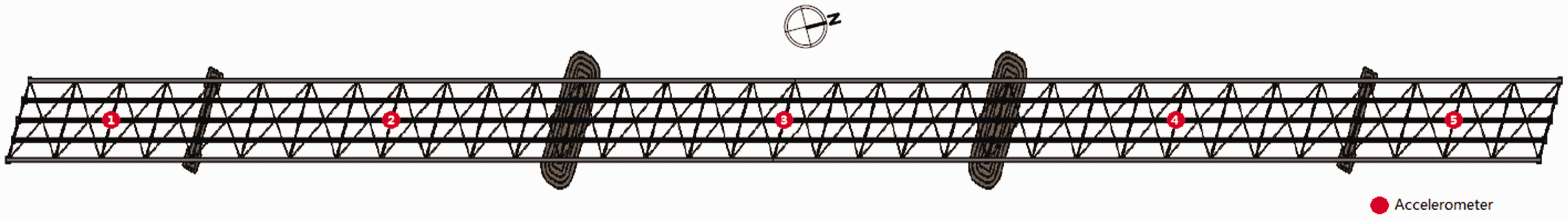
Plan view road deck hidden.

Figure 6.

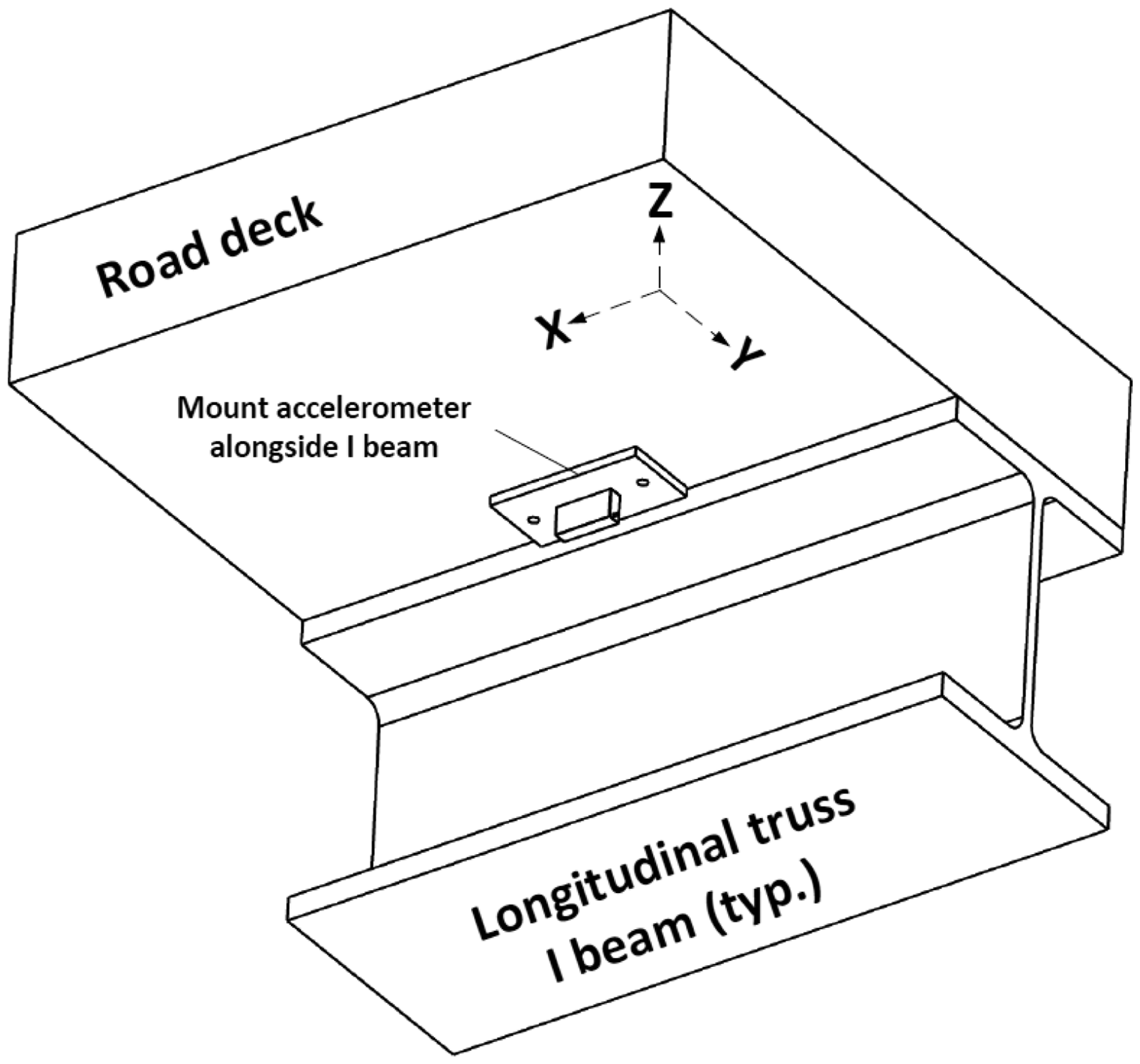
Accelerometer at the bottom of the bridge deck.

Spectrum analysis

In the following analysis, we only chose one representative piece of data for processing. Figure 7 shows the acceleration signal recorded at location number 1 (Figure 5). The trucks entered the bridge approximately 1.6 s, and the bridge remained closed until the vibrations damped out. Figures 8 and 9 show two kinds of power spectrum. Figure 10 shows the 3 D spectrogram, and Figure 11 shows the scalogram.

Figure 7.

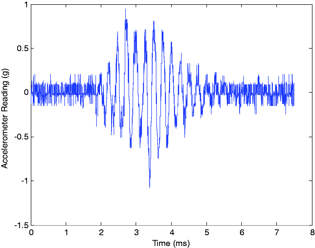
Response of the accelerometer.

Figure 8.

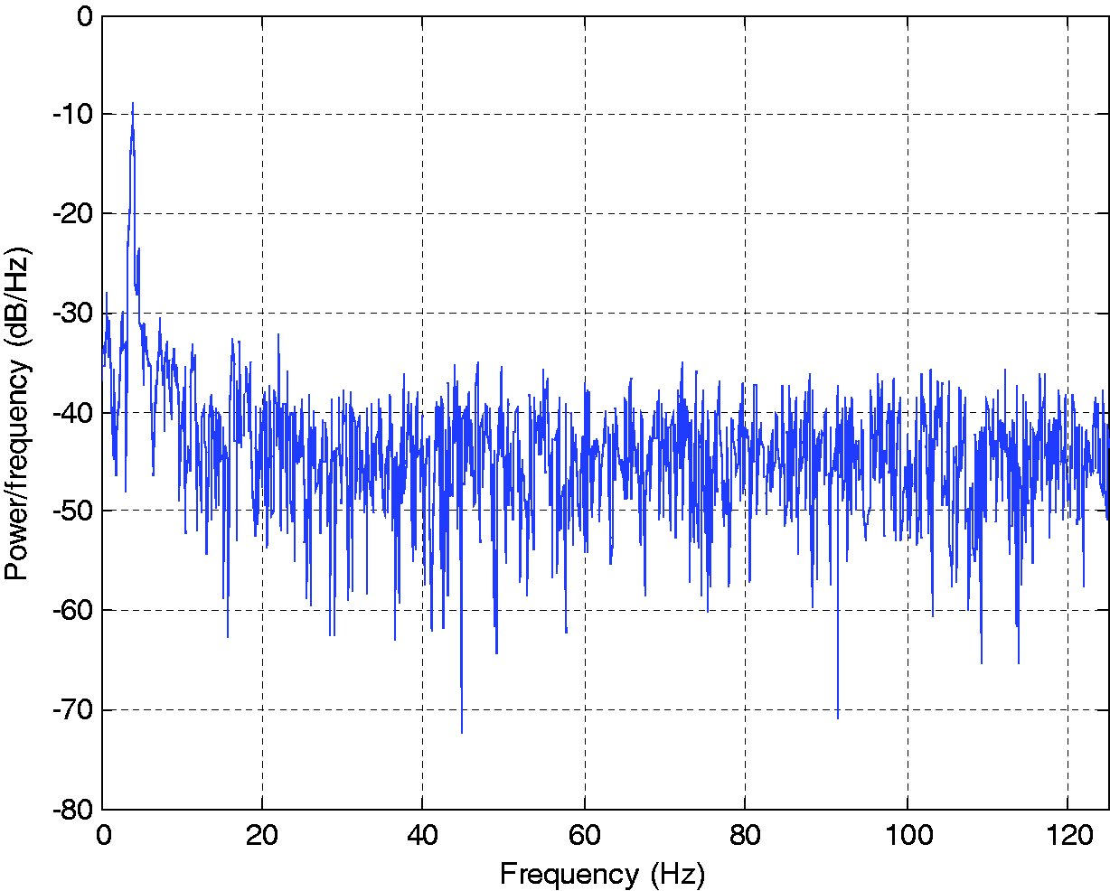
Periodogram power spectral density.

Figure 9.

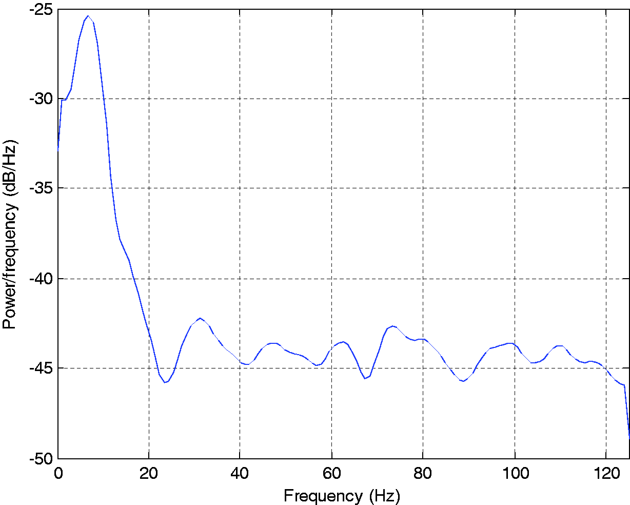
Welch power spectral density estimate.

Figure 10.

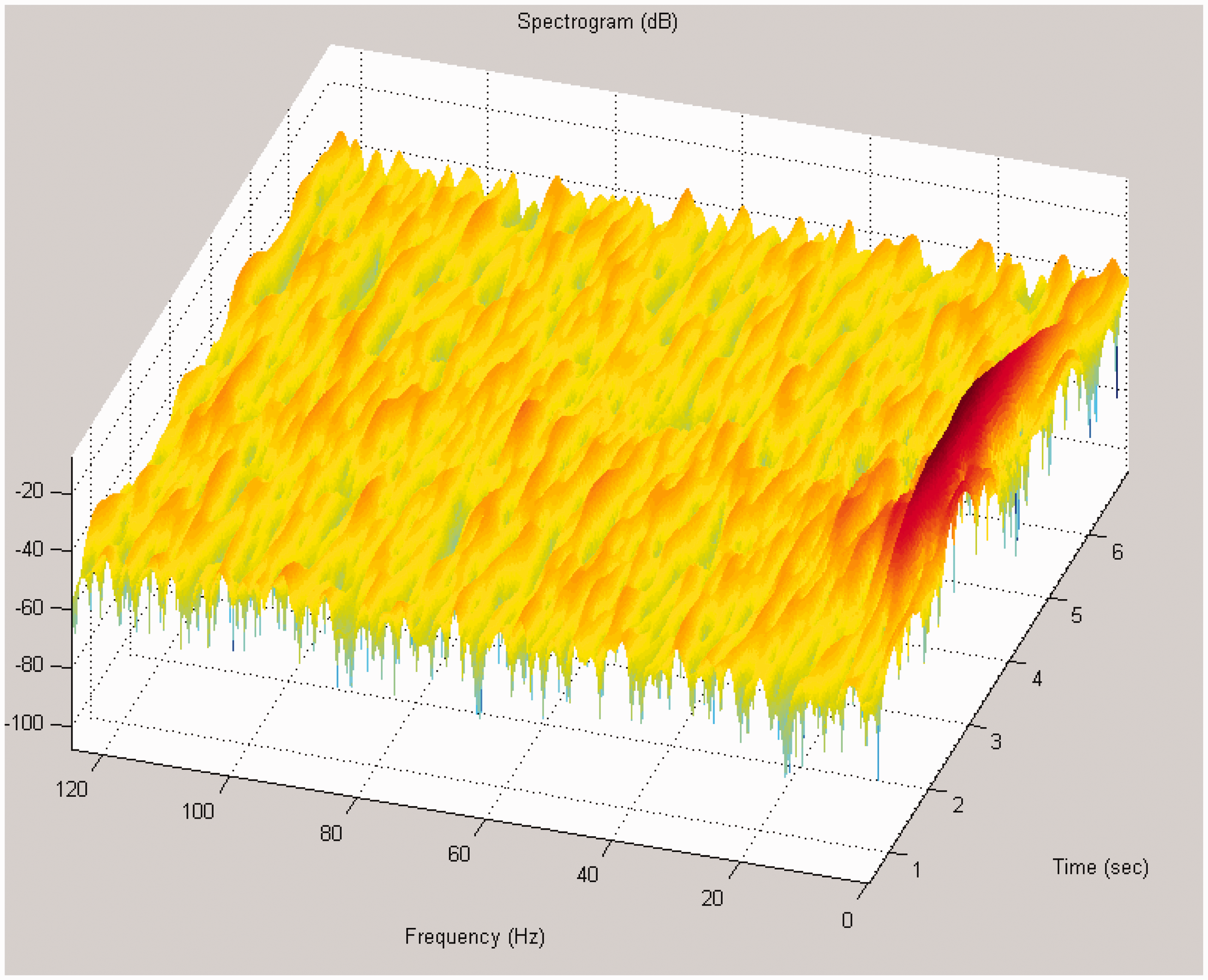
Three-dimensional spectrogram.

Figure 11.

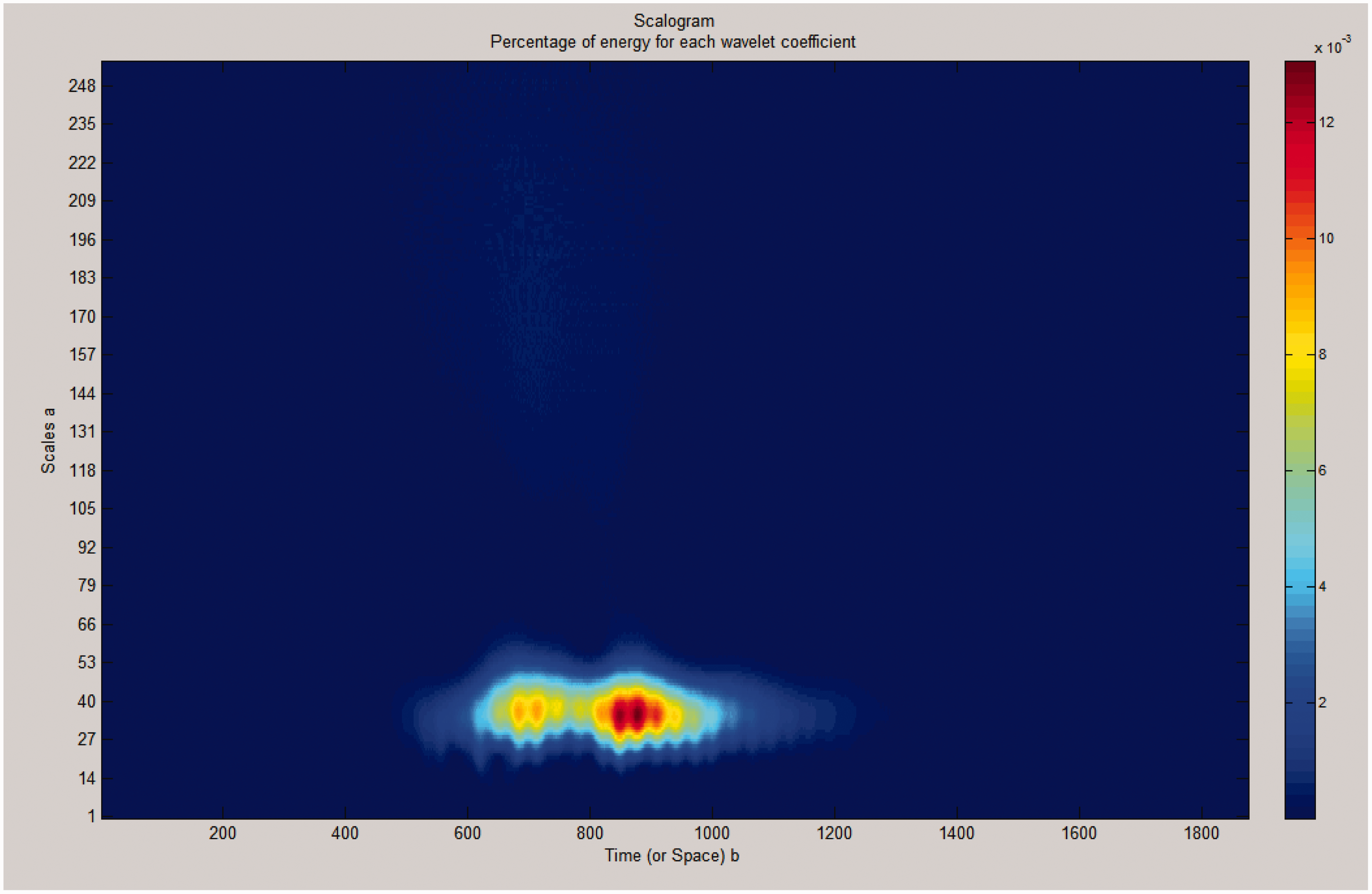
Scalogram.

From these results, we can see that all those kinds of spectrum have merged components that are not correlated with the modes from FEM. Next, we use the EMD method to extract the specific signal and identify the system’s specific spectrum signatures.

EMD analysis and parameter estimates

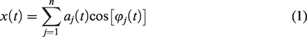
To decompose the signal into its time–frequency expression as in Figure 7, in the next step, we use an EMD method to decompose the response signal. Before presenting the results, the basic formulations used for EMD are introduced as follows. EMD is a method of decomposing a nonlinear and nonstationary signal into a series of zero-mean amplitude-modulation frequency-modulation (AM–FM) components that represent the characteristic time scale of the observation. A multicomponent AM–FM model for a nonlinear and nonstationary signal, x(t), can be represented as

x (t) = \sum_{j = 1}^{n} a_{j} (t) \cos [φ_{j} (t)]

(1)

where a_j(t) and

φ_{j} (t)

represent the instantaneous amplitude and the instantaneous phase of the jth component, and n is the number of components. In the EMD approach, this is done by iteratively conducting a sifting process. The zero-mean AM–FM components are called IMFs, which must satisfy the following requirements: (1) the number of extremes and the number of zero crossings in the IMF must either be equal or differ at most by one and (2) at any point the mean value of the envelopes defined by the local maxima and local minima must be zero. In short, the signal is locally symmetric around the time axis. The sifting process for finding IMFs for the signal x(t) consists of the following steps:

1) Find the positions and amplitudes of all the local maxima and all the local minima in the input signal x(t). Then, create an upper envelope by cubic spline interpolation of the local maxima and a lower envelope by cubic spline interpolation of the local minima. Calculate the mean of the upper and lower envelopes; this is defined as m₁(t). Subtract the mean envelope signal, m₁(t), from the original input signal

h (t) = x (t) - m_{1} (t)

(2)

Check whether h(t) meets the requirements to be an IMF. If not, treat h(t) as new data and repeat the previous process. Then, set

h_{11} (t) = h_{1} (t) - m_{11} (t)

(3)

Repeat this sifting procedure k times until h₁ _k (t) is an IMF; this is designated as the first IMF

c_{1} (t) = h_{1 k} (t)

(4)

2) Subtract c₁(t) from the input signal and define the remainder, r₁(t), as the first residue. Since the residue, r₁(t), still contains information related to the longer period components, treat it as a new data stream and repeat the above-described sifting process. This procedure can be repeated j times to generate j residues, r_j(t), (j = 1, 2, …, n), resulting in

{\begin{matrix} r_{1} (t) - c_{2} (t) = r_{2} (t) \\ ⋮ \\ r_{n - 1} (t) - c_{n} (t) = r_{n} (t) \end{matrix}

(5)

The sifting process is stopped when either of two criteria is met: (1) the component c_n(t), or the residue $r_{n} (t)$ , becomes so small as to be considered inconsequential, or (2) the residue, $r_{n} (t)$ , becomes a monotonic function from which an IMF cannot be extracted. By summing equations (4) and (5), the original signal can be reconstructed using the resulting IMFs and the final residue

x (t) = \sum_{j = 1}^{n} c_{j} (t) + r_{n} (t)

(6)

Next, apply the Hilbert transform to all IMFs, $c_{j} (t)$ in equation (6), to derive model parameters including frequency and damping

H [c_{j} (t)] = \frac{1}{π} \int_{- \infty}^{\infty} \frac{c_{j} (t)}{t - τ} d τ

(7)

After the Hilbert transform, $H [c_{j} (t)]$ and c_j(t) form a complex signal $Z_{j} (t)$

Z_{j} (t) = c_{j} (t) + i H [c_{j} (t)] = a (t) e^{i φ (t)}

(8)

Then, the envelope of every IMF can be given by

a_{j} (t) = \sqrt{{[c_{j} (t)]}^{2} + H [c_{j} (t)]}, φ_{j} (t) = \arctan {H [c_{j} (t)] / c_{j} (t)}

(9)

In which $a_{j} (t)$ , the instantaneous amplitude of x(t), reflects how the energy of x(t) varies with time. The term $φ_{j} (t)$ is the instantaneous phase of x(t). The instantaneous frequency $ω (t)$ is defined as the time derivative of the instantaneous phase $φ (t)$ as follows

ω (t) = \frac{d φ (t)}{d t}

(10)

Then, the original signal x(t) can be expressed as

x (t) = \sum_{j = 1}^{n} a_{j} (t) \exp [i \int^{​} ω_{j} (t) d t]

(11)

However, some problems in EMD remain unaddressed, among which mode mixing is the most serious. To solve the mode mixing problem, an EEMD algorithm was introduced.¹⁴ Although EEMD alleviates the effect of mode mixing, noise will remain in the corresponding IMF(s) if the ensemble number is small. To ensure a noise-free IMF, a CEEMD algorithm¹⁷ is introduced. The previous method leads to a new problem, which is the high computational load for CEEMD decomposition. To reduce the computational cost and retain the ability to eliminate mode mixing, a CEEMDAN algorithm is proposed.¹⁹ The steps of CEEMDAN decomposition are as follows:

Decompose the signal $x (t) + w_{0} ε^{i} (t)$ to obtain the first mode by using the EMD algorithm

c_{1} (t) = \frac{1}{N} \sum_{i = 1}^{N} c_{1}^{i} i \in {1 \dots N}

(12)

where $w_{0}$ is the amplitude of the added white noise, N is the ensemble number, and $ε (t)$ is the white noise with unit variance. It should be noted that here the mean of the corresponding IMFs is used as the final signal IMF.

2. Compute the difference signal

r_{1} (t) = x (t) - c_{1} (t)

(13)

3. Assume $E_{1} (\cdot)$ represents a function for extracting the first IMF decomposed by EMD. Decompose $r_{1} (t) + w_{1} E_{1} (ε^{i} (t))$ to obtain the first mode IMF and define the second mode by

c_{2} (t) = \frac{1}{N} \sum_{i = 1}^{N} E_{1} (r_{1} (t) + w_{1} E_{1} (ε^{i} (t)))

(14)

4. For $k = 2, \dots, K$ , calculate the kth residue and obtain the first mode. Define the (k + 1)th mode as follows

c_{k + 1} (t) = \frac{1}{N} \sum_{i = 1}^{N} E_{1} (r_{k} (t) + w_{k} E_{k} (ε^{i} (t)))

(15)

where $E_{j} (\cdot)$ is a function to extract the jth IMF decomposed by EMD, and $w_{k}$ is the amplitude of the added white noise for a specific signal-noise-ratio.¹⁹

5. Repeat Step 4 until the residue contains no more than two extrema. The residue mode is then defined as

R (t) = x (t) - \sum_{k = 1}^{K} c_{k} (t)

(16)

Therefore, the signal x(t) can be expressed as follows

x (t) = \sum_{k = 1}^{K} c_{k} (t) + R (t)

(17)

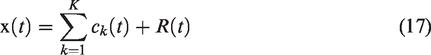
Figure 12 illustrates a flowchart of the CEEMDAN method.

Figure 12.

Flowchart of CEEMDAN method. IMF: intrinsic mode function.

Next, we illustrate the results of EMD decomposition and spectrum identification using a typical measured acceleration signal as shown in Figure 7. Figure 13 shows the decomposed components of the measured acceleration signal. Figure 14 shows the Hilbert spectrum of the IMFs, and Amp means amplitude of spectrum.

Figure 13.

Decomposed components of a measured acceleration signal using the EMD method. IMF: intrinsic mode function.

Figure 14.

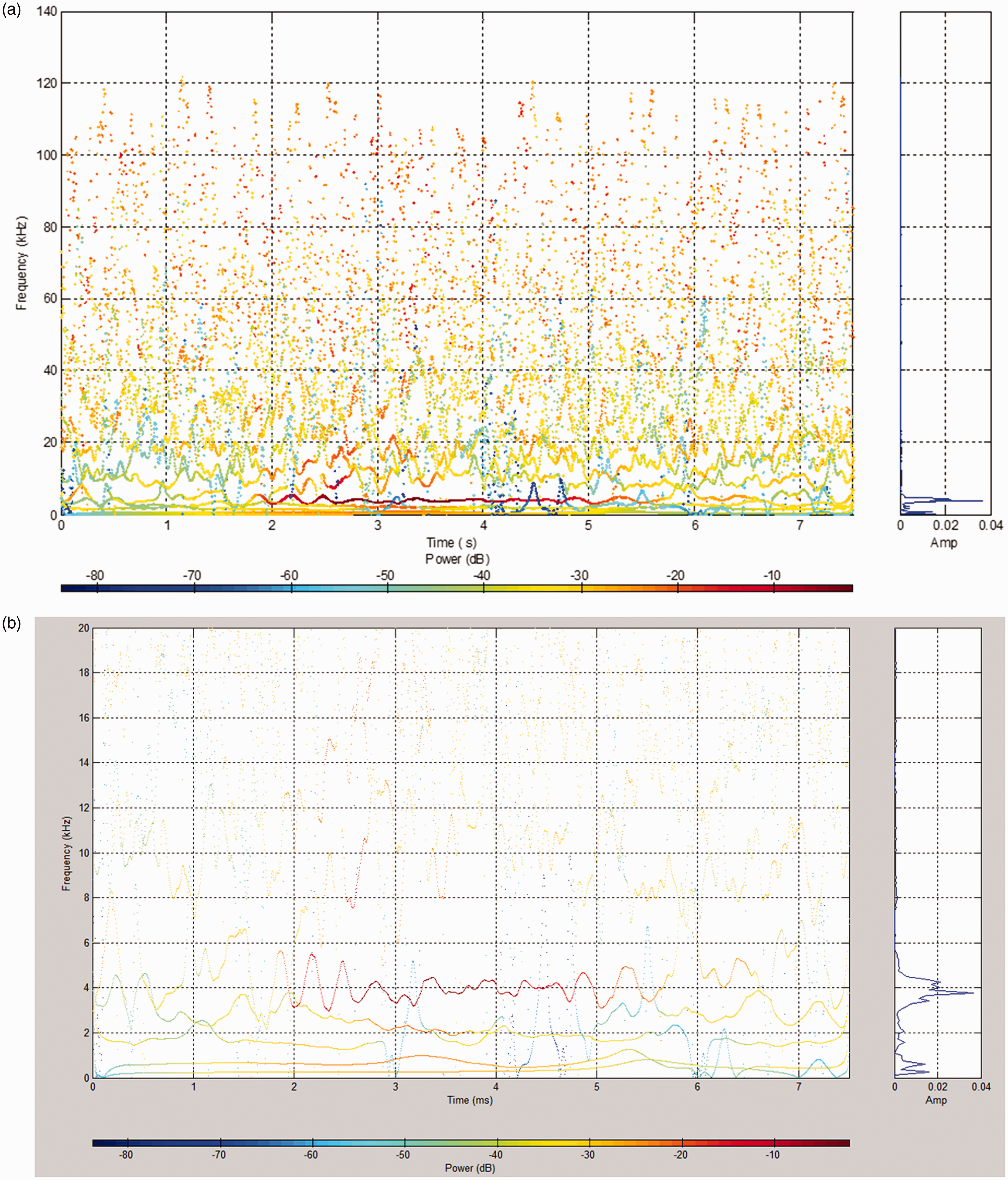
EMD HHT results.

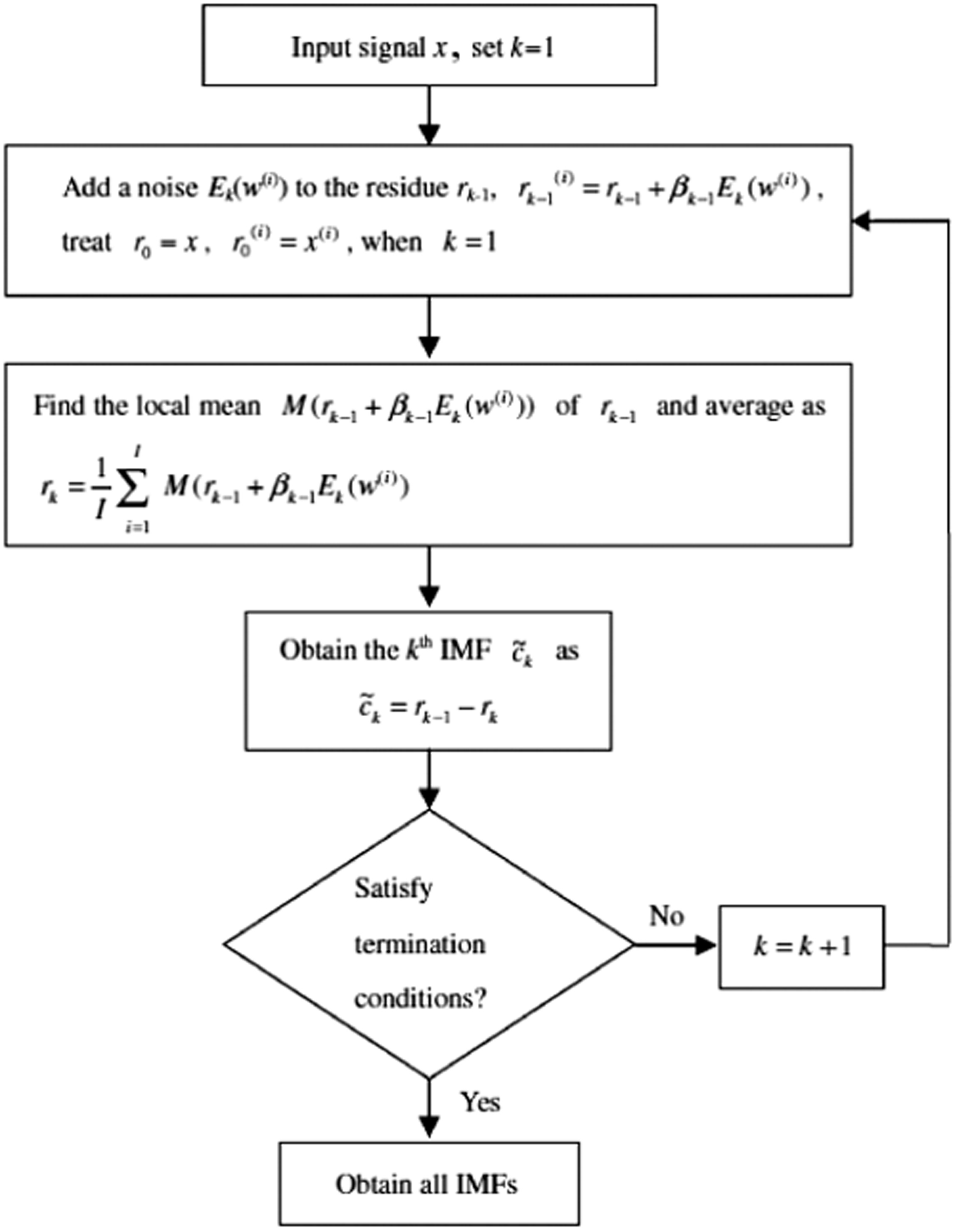
Next, we illustrate the results of CEEMDAN decomposition and spectrum identification using a typical measured acceleration signal as shown in Figure 7. Figure 15 shows the decomposed components of the measured acceleration signal. Boxplots of the sifting iterations required by each decomposition are presented in Figure 16. Figure 17 shows the Hilbert spectrum of the IMFs.

Figure 15.

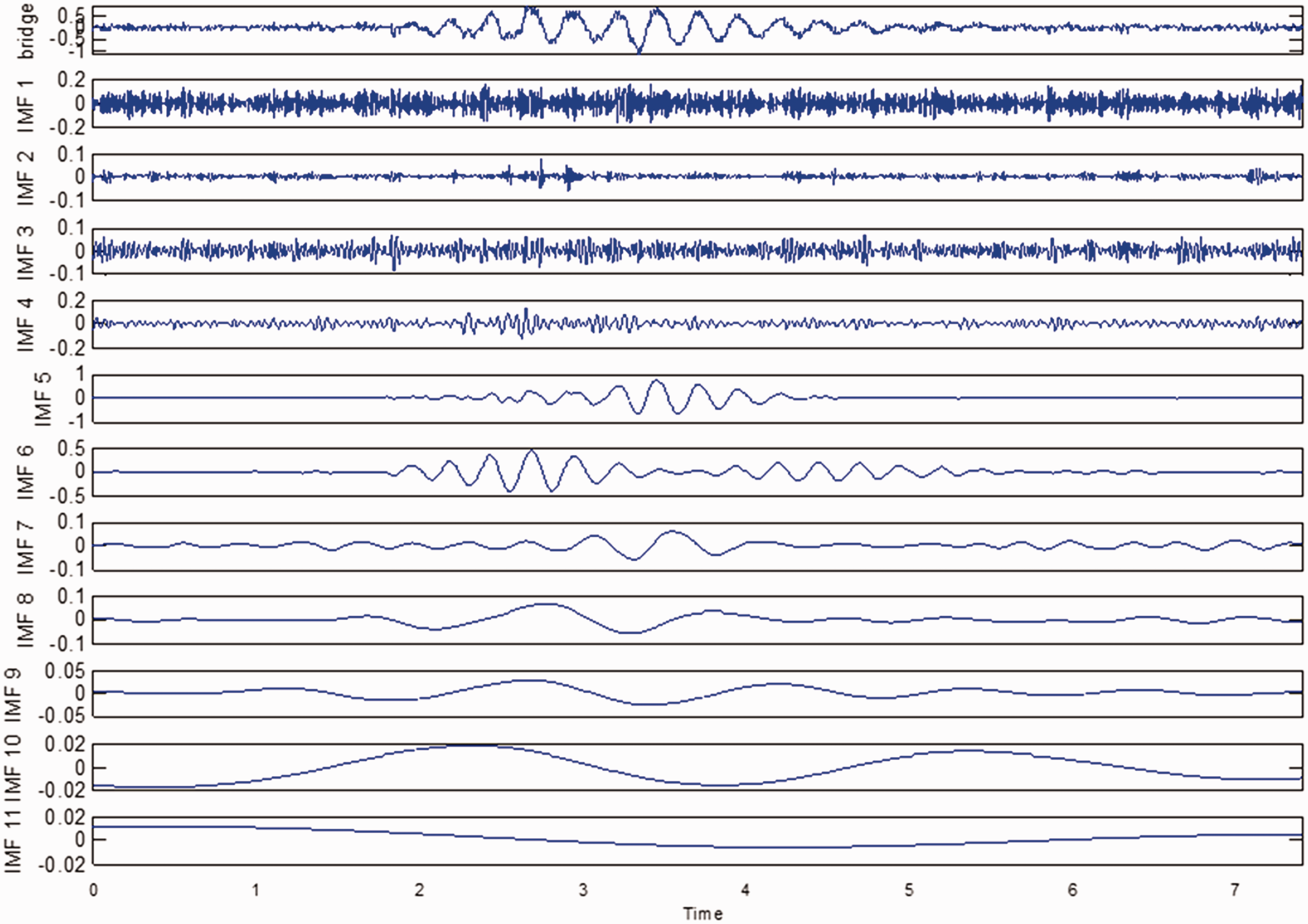
Decomposed components of a measured acceleration signal using CEEMDAN results. IMF: intrinsic mode function.

Figure 16.

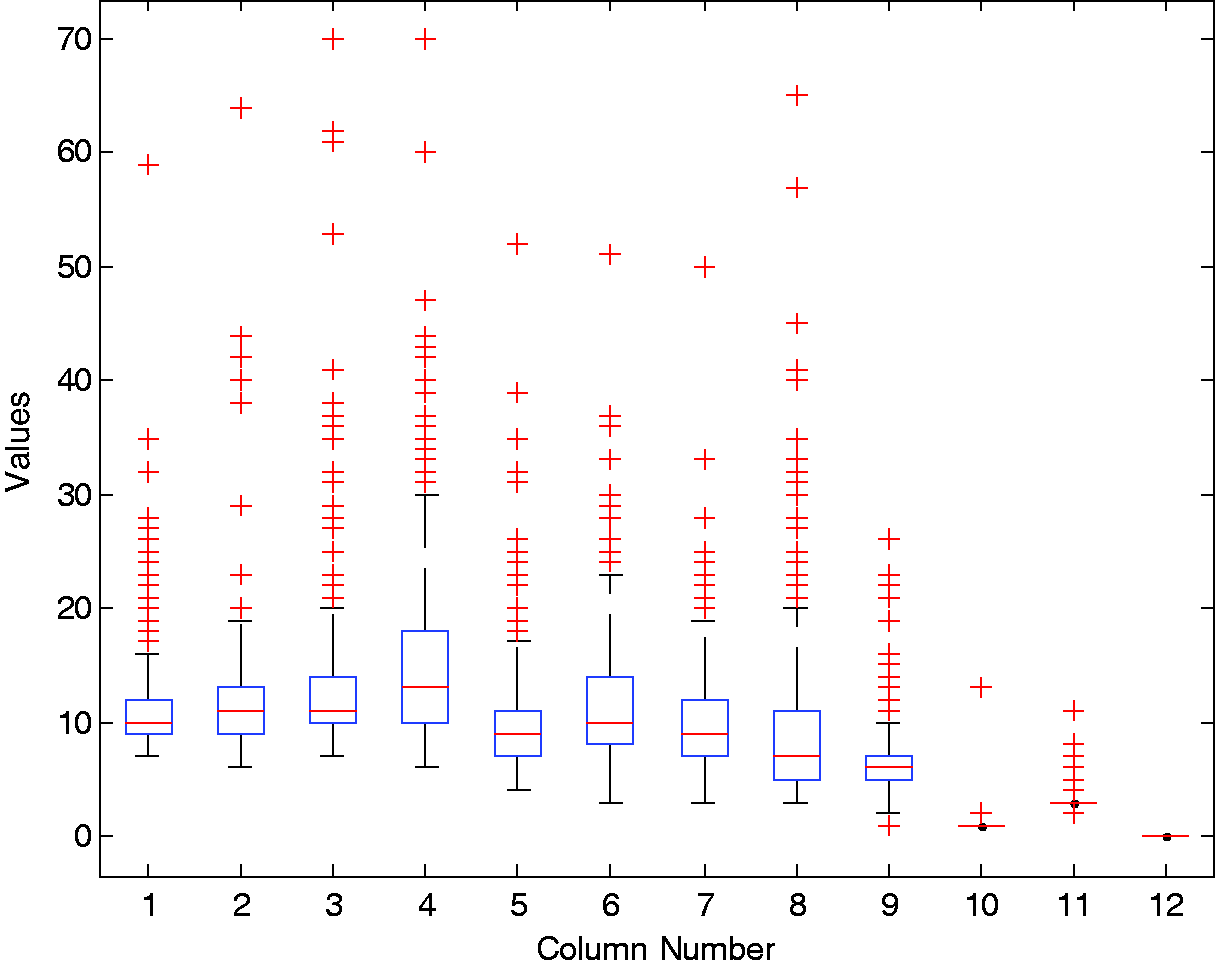
Boxplots showing the sifting iterations for each mode.

Figure 17.

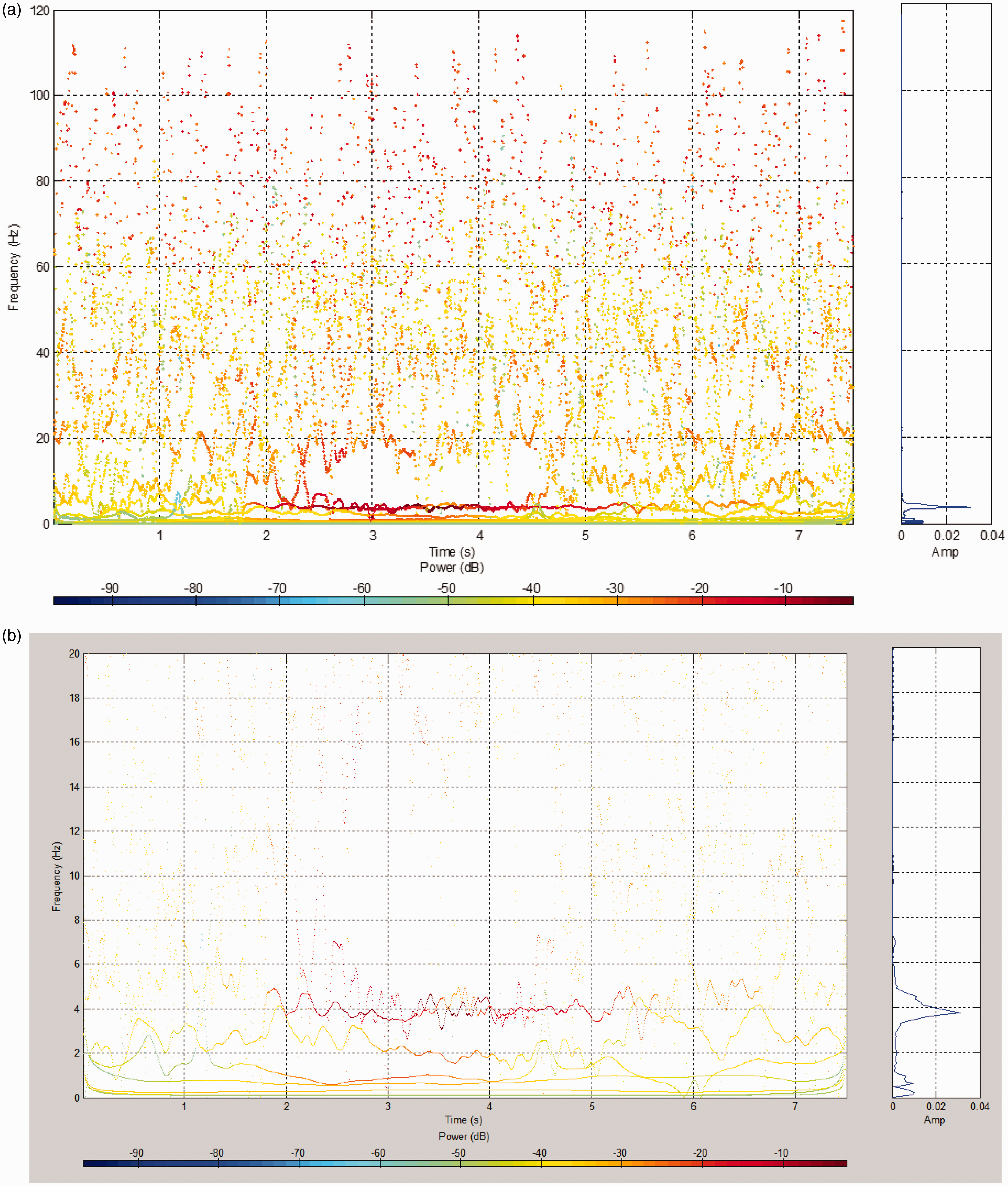
CEEMDAN HHT results.

Discussion and theoretical consideration

The approximate FEM results in Table 1 are based on linear mode analysis. It should be noted that in principle, a real bridge system under a moving vehicle is time varying. Many factors could result in variation in specific transient mode frequencies, such as vehicle motion and location, road excitation due to roughness/bumpiness, etc. Both spectrograms and scalograms exhibit mode mixing and merging in the proximity of linear natural frequencies (2.8–4.2 Hz) as shown in Table 1. However, in the proximity of these linear mode frequencies, both EMD and CEEMDAN give rise to clear transient frequencies with high resolution, which are superior to the results from power spectra, spectrograms, and scalograms. The HHT method does not suffer from the limitations of linearity required by the Fourier transform and its extensions. EMD generates adaptive basis IMFs from the signal. EMD is a method for decomposing a nonlinear and nonstationary signal into a series of zero-mean AM–FM components that represent the characteristic time scale of the observation. This is done by iteratively conducting a sifting process. Based on the analysis, the level of nonstationary and nonlinear features can be estimated. The advantage of CEEMDAN is that it has been theoretically proven and verified by many applications in other communities. We demonstrated that the bridge response identified using CEEMDAN is different from the results obtained from EMD. By comparing the dominant transient modes in Figures 14 and 17 in the range of 2–5 s, we can see that the spectrum results from EMD exhibit frequency variation between 3 and 5.5 Hz, whereas the spectrum results from CEEMDAN give rise to frequency variation between 3.5 and 5 Hz. This results in a 17% difference at the low-end and a 10% difference at the high-end.

SHM requires estimating the state of a bridge from the measured acceleration and the system’s identification. Conventional approaches involve estimation and identification of the system’s natural modes such as its frequency and natural modes as characterized in linear finite element analysis. However, real bridge responses exhibit complex dynamical properties including time-varying patterns. One specific aspect of SHM bridge studies is the characterization of the bridge’s time-varying responses under passing vehicles. Compared with conventional time–frequency spectrum approaches, CEEMDAN exhibits high resolution, and compared with other existing EMD approaches, CEEMDAN exhibits salient differences and its accuracy is guaranteed by an existing theoretical proof. As such, the time–frequency spectrum of CEEMDAN can be reliably applied as a signature for bridge SHM.

Conclusions

In this paper, CEEMDAN is applied for the first time to characterize the acceleration response of a bridge to a moving vehicle to extract the spectrum signatures of the bridge. The results of CEEMDAN are more adaptive and are obviously better than conventional power spectra, spectrograms, and scalograms in resolution. Both EMD and CEEMDAN offer very good resolution for transient frequency spectra. However, the results of the Hilbert spectrum of CEEMDAN are different from those of EMD, with a more than 10% difference in the estimated specific transient frequencies. CEEMDAN has been theoretically proven to be superior to EMD, as the results from EMD have a mode mixing problem and are therefore not as reliable as CEEMDAN results.

Footnotes

Acknowledgements

The writers wish to acknowledge the support from the Alaska Department of Transportation & Public Facilities, University of Alaska Fairbanks, University of Alaska Anchorage, Alaska Native Science and Engineering Program, Chandler Monitoring System Inc., Micron Optic, Inc.

Declaration of conflicting interests

The author(s) declared no potential conflicts of interest with respect to the research, authorship, and/or publication of this article.

Funding

The author(s) disclosed receipt of the following financial support for the research, authorship, and/or publication of this article: This work was supported by the Alaska University Transportation Center Grant No. 510015 and Nanjing University of Science and Technology, Start‐up, Grant Number: AE89991.

References

Zhu

Law

SS.

Structural health monitoring based on vehicle-bridge interaction: accomplishments and challenges.

Adv Struct Eng 2015; 18: 1999–2015.

Cantero

Obrien

EJ.

The non-stationarity of apparent bridge natural frequencies during vehicle crossing events. FME Trans 2013; 41: 279–284.

Hester D and Gonzále A. A discussion on the merits and limitations of using drive-by monitoring to detect localised damage in a bridge. Mech Syst Signal Process 2017; 90: 234–253.

Mahato

Vinay Teja

Chakraborty

Combined wavelet–Hilbert transform-based modal identification of road bridge using vehicular excitation.

J Civil Struct Health Monit 2017; 7: 29–44.

Malekjafarian

Obrien

EJ.

On the use of a passing vehicle for the estimation of bridge mode shapes. J Sound Vib 2017; 397: 77–91.

Huffman

Xiao

Chen

, et al. Detection of soil-abutment interaction by monitoring bridge response using vehicle excitation. J Civil Struct Health Monit 2015; 5: 389–395.

Hlawatsch

Boudreaux-Bartels

GF.

Linear and quadratic time-frequency signal representations. IEEE Signal Process Mag 1992; 9: 21–67.

Huang

Shen

Long

, et al. The empirical mode decomposition and the Hilbert spectrum for nonlinear and nonstationary time series analysis. Proc R Soc Lond A 1998; 454: 903–995.

Smith

The local mean decomposition and its application to EEG perception data. J R Soc Interface 2005; 2: 443–454.

10.

Rioul

Flandrin

Time scale energy distributions: a general class extending wavelet transforms. IEEE Trans Signal Process 1992; 40: 1746–1757.

11.

Cohen

Time-frequency distributions-a review. Proc IEEE 1989; 77: 941–981.

12.

Poyil

Aljahdali

Nasimudeen

KM.

Significance of Cohen’s class for time frequency analysis of signals. Int J Comput Appl 2013; 72(12): 1–12.

13.

Baraniuk

Jones

DL.

Signal-dependent time frequency representation: optimal kernel design. IEEE Trans Signal Process 1993; 41: 1589–1602.

14.

Huang

NE.

Ensemble empirical mode decomposition: a noise-assisted data analysis method. Adv Adapt Data Anal 2009; 1: 1–41.

15.

Fang

Y-M

Feng

H-L

, et al. Stress wave signal denoising using ensemble empirical mode decomposition and an instantaneous half period model. Sensors 2011; 11: 7554–7567.

16.

Goubran

Liu

XP.

Ensemble empirical mode decomposition and adaptive filtering for ECG signal enhancement. In: Proceedings of 2012 IEEE international symposium on medical measurements and applications (MeMeA), Budapest, Hungary, 18–19 May 2012, pp.1–5.

17.

Yeh

J-R

Shieh

J-S

Huang

NE.

Complementary ensemble empirical mode decomposition: a novel noise enhanced data analysis method. Adv Adapt Data Anal 2010; 2: 135–156.

18.

Wang

Ferreira

VG.

Ocean wave separation using CEEMD-wavelet in GPS wave measurement. Sensors 2015; 15: 19416–19428.

19.

Torres

Colominas

Schlotthauer

, et al. A complete ensemble empirical mode decomposition with adaptive noise. In: Proceedings of 2011 IEEE international conference on acoustics, speech and signal (ICASSP), Prague, Czech, 22–27 May 2011, pp.4144–4147.

20.

Loomis

Luthcke

SB.

Optimized signal denoising and adaptive estimation of seasonal timing and mass balance from simulated GRACE-like regional mass variations. Adv Adapt Data Anal 2014; 6: 1450003.

21.

Humeau-Heurtier Abraham

Mahé

PG.

Analysis of laser speckle contrast images variability using a novel empirical mode decomposition: comparison of results with laser Doppler flowmetry signals variability. IEEE Trans Med Imaging 2015; 34: 618–627.

22.

Marusiak

Pekar

Analysis of multiannual fluctuations and long term trends of hydrological time series. In: Advances in environmental sciences, development and chemistry, Greece, 2014.

23.

Hassan

Haque

MA.

Epilepsy and seizure detection using statistical features in the complete ensemble empirical mode decomposition domain. In: TENCON 2015-2015 IEEE region 10 conference, 1 November 2015, pp.1–6. Piscataway, NJ: IEEE.

24.

Antico

Schlotthauer

Torres

ME.

Analysis of hydroclimatic variability and trends using novel empirical mode decomposition: application to the Paraná River Basin. J Geophys Res Atmos 2014; 119: 1218–1233.

25.

Lei

Liu

Ouazri

, et al. A fault diagnosis method of rolling element bearings based on CEEMDAN. Proc IMechE, Part C: J Mechanical Engineering Science 2017; 231: 1804–1815.

26.

Pretreatment and wavelength selection method for near-infrared spectra signal based on improved CEEMDAN energy entropy and permutation entropy. Entropy

2017; 19: 380.

27.

Elouaham

Dliou

Latif

, et al. Filtering of biomedical signals by using complete ensemble empirical mode decomposition with adaptive noise. Int J Comput Appl 2016; 149: 39.

28.

Chen

, et al. Monitoring temperature effect on a long suspension bridge. Struct Control Health Monit 2010; 17: 632–653.

29.

Xia

Chen

Zhou

, et al. Field monitoring and numerical analysis of Tsing Ma suspension bridge temperature behavior. Struct Control Health Monit 2013; 20: 560–575.

30.

Chen

Zhang

RC.

Modal parameter identification of Tsing Ma suspension bridge under Typhoon Victor: 20 mathematical problems in engineering EMD-HT method. J Wind Eng Ind Aerodyn 2004; 92: 805–827.

31.

Ren

WX.

EMD-based stochastic subspace identification of structures from operational vibration measurements. Eng Struct 2005; 27: 1741–1751.

32.

Han

Modal parameter identification of civil engineering structures based on Hilbert-Huang transform. Eng Struct Integr Res Dev Appl 2007; 1–2: 366–368.

33.

Huang

SX.

Engineering of civil “Application of Hilbert-huang Transform to Identify Modal Parameters for Large Bridge”. In: Proceedings of the 4th international symposium on lifetime infrastructure, 2009, pp.478–481.

34.

Hua

Chen

, et al. EMD-based random decrement technique for modal parameter identification of an existing railway bridge. Eng Struct 2011; 33: 1348–1356.

35.

Qin

Wang

Kang

Output-only modal analysis based on improved empirical mode decomposition method. Adv Mater Sci Eng. Epub ahead of print 2015. DOI: 10.1155/2015/945862.

36.

Wang

Liu

JK.

Time-frequency analysis of a coupled bridge-vehicle system with breathing cracks. Interact Multiscale Mech 2012; 5: 169–185.

37.

Hester

González

Application of empirical mode decomposition to drive-by bridge damage detection. J Mech A/Solids 2017; 61: 151–163

38.

Kunwar

Jha

Whelan

, et al. Damage detection in an experimental bridge model using Hilbert–Huang transform of transient vibrations. Struct Control Health Monit 2013; 20: 1–15.

39.

Zhang

Wang

The advanced Hilbert-Huang transform using in bridge micro-Doppler phenomenon. J Residuals Sci Technol 2016; 13: 55.1.

40.

Aied

González

Cantero

Identification of sudden stiffness changes in the acceleration response of abridge to moving loads using ensemble empirical mode decomposition. Mech Syst Signal Process 2016; 66–67: 314–338.

41.

Xiao

Chen

Hulsey

, et al. Ambient loading and modal parameters for the Chulitna River Bridge. Adv Struct Eng 2016; 19: 660–670.

42.

Xiao F, Hulsey JL, Balasubramanian R. Fiber optic health monitoring and temperature behavior of bridge in cold region. Struct Control Health Monit 2017; 24(11): e2020. DOI: 10.1002/stc.2020

43.

Micron Optics, Inc. os7100 Accelerometer, http://www.micronoptics.com/product/accelerometer-os7100/ (accessed 31 October 2017).

Signature extraction from the dynamic responses of a bridge subjected to a moving vehicle using complete ensemble empirical mode decomposition

Abstract

Keywords

Introduction

Bridge description

Testing of the bridge under passing vehicle

Spectrum analysis

EMD analysis and parameter estimates

Discussion and theoretical consideration

Conclusions

Footnotes

Acknowledgements

Declaration of conflicting interests

Funding

References