
Abstract
As an important research direction for the future innovation and development of the energy industry, integrated energy system (IES) requires short-term load forecasting as the decision-making basis. A short-term load forecasting model based on improved complete ensemble empirical mode decomposition with adaptive noise (ICEEMDAN) maximum information coefficient (MIC) transformer is proposed to address the problem of high volatility and strong randomness in IES short-term load. The model effectively reduces the complexity of time series and alleviates the impact of modal aliasing by ICEEMDAN. Perform correlation analysis and reconstruction of the decomposed intrinsic mode function using MIC to improve the coupling relationship between multivariate loads. Finally, Transformer model based on self-attention mechanism is used to predict each component and obtain the final prediction result. The horizontal comparison experiment and vertical ablation experiment were conducted on the model using the IES dataset from Arizona State University in the United States. The results showed that the predictive performance of the model was improved to a certain extent and it had a certain degree of application prospects.
Keywords
Introduction
In recent years, new energy technology has continued to progress and iterative updating. A new model of energy consumption, with renewable and clean energy as an important guide and key benchmark, is also being gradually formed and improved (Lilhore et al., 2025; Simaiya et al., 2024; Sunder et al., 2024). Against the background of abundant energy supply and diversified energy demand, the concept of integrated energy system (IES) has been proposed and has become a research hotspot in the energy field in recent years (Chowdary et al., 2025). Overall, IES takes the electric power system as the core, utilizes various types of energy equipment with complex functions, and breaks down the interaction barriers between different energy systems. IES realizes integrated planning and collaborative management on the whole, and optimized operation and coordination and stability on the local level (Alofaysan et al., 2024). Specifically, for the energy demand of users in production and life of cold, heat, gas and electricity, the energy supplier adjusts the energy planning and supply proportion according to the target macro and micro factors, so as to achieve rationalization, high efficiency and coordinated scheduling of regional energy. Therefore, the development of IES not only puts forward higher requirements for energy generation, transmission, transformation and storage in the process of multivariate load interaction, but also poses a great challenge to the speed of energy information exchange and processing capability.
As the decision support for IES energy and communication interaction, the accuracy and response time of short-term load forecasting will have an impact on the whole IES. Unlike single load, load forecasting under IES should further consider the coupling relationship between multivariate energy sources and improve the accuracy of multi-energy load forecasting, thus enabling energy suppliers to realize the fine-grained scheduling of integrated energy sources (Gielen et al., 2019). As shown in Figure 1, by utilizing equipment such as chillers, electric heat pumps, cogeneration, combined heat and power units, gas boiler and electric gas conversion (P2G) systems, and fuel cells, energy suppliers can jointly dispatch integrated energy sources at the district level according to the multivariate energy demands of users, increasing the overall energy use efficiency and reducing unnecessary losses (Smeers et al., 2021).
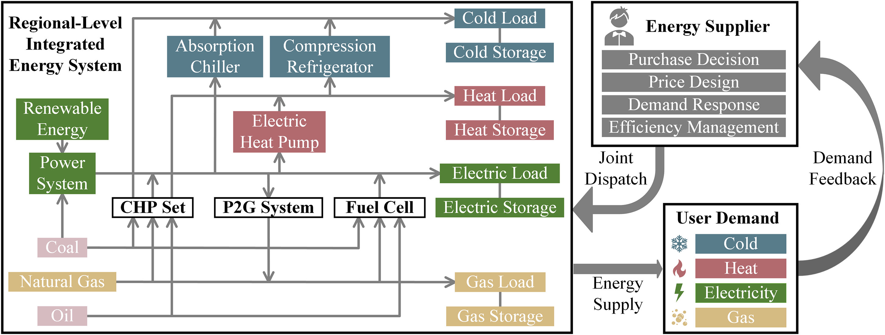
The interaction structure of integrated energy system (IES) energy and information.
Since the concept of IES was proposed late, most of the IES load forecasting models are based on deep learning models with strong nonlinear function fitting capability. Yujie et al. proposed a vector auto regressive based IES load forecasting method has been proposed (Li et al., 2018). They consider the correlation between electricity, gas, and cold loads, and adds temperature as an external variable for load prediction. A model for short-term dual load demand forecasting of electricity and gas has been proposed by Tang et al., which is based on radial basis function neural network (RBF-NN) (Tang et al., 2019). This model fully considers the coupling relationship of loads and strengthens the spatiotemporal correlation by adding electricity price factors. Then use the RBF-NN model to predict the two types of loads separately. Due to the increasing amount of IES data, models with larger scales and deeper layers are being applied. Xuan et al. utilized three different structures of models, namely convolutional neural network (CNN), gated recurrent unit (GRU), and gradient boosting regressor tree, to form a multivariate load forecasting model (Wang et al., 2021). Zhang et al. proposed a load forecasting method based on deep belief network (DBN) and multivariate task regression layers, which was applied to electricity, heat, and gas energy prediction. In order to extract hidden features from multivariate load time series, Zhou et al. proposed another prediction model based on DBN, which achieved net load prediction for both producers and consumers (Zhou et al., 2021).
Transformer was proposed in reference Vaswani et al. (2017) and subsequently applied in various industries. Wang et al. improved the basic model and proposed a short-term load forecasting model for IES (Wang et al., 2022). This model utilizes self-attention mechanism to effectively couple the relationship between electricity, cold, and heat loads, achieving the goal of synchronous input/output. The experimental results show that this method has better predictive performance compared to traditional methods.
In this study, we propose a IES short-term load forecasting model based on improved complete ensemble empirical mode decomposition with adaptive noise (ICEEMDAN) maximum information coefficient (MIC) transformer that achieves the high precision synchronous prediction of short-term load time series in IES. Considering the volatility and randomness of IES short-term load time series, the signal decomposition algorithm is used to effectively decompose the original signal. As a cutting-edge algorithm in time series decomposition, ICEEMDAN has excellent performance in reducing signal complexity. For the decomposed intrinsic mode function (IMF) components, use the MIC algorithm for correlation analysis and reconstruction. The reconstructed multivariate load data is used as the input of the encoder, and the single load data is used as the input of the decoder, synchronously outputting the multivariate prediction score and obtain the final result.
The rest of this article is organized as follows. The “Methodology” section introduces the algorithms and models used in this article. The “Data analysis and index description” section provides a brief analysis and description of the IES dataset and evaluation metrics. The experimental results and analysis are presented in The “Result analysis” section. The “Conclusion” section provides a summary of the entire text.
Methodology
ICEEMDAN Algorithm
The energy use behavior of energy users changes over time, so load signals are typical time series signals. This type of time series signal possesses high complexity and randomness. A common method used by researchers to effectively reduce this type of complexity and randomness is to split the original signal into several IMFs using decomposition methods. As a classical adaptive decomposition method, empirical modal decomposition (EMD) is good at handling nonlinear and nonsmooth data (Wang et al., 2022). Therefore, EMD has also been applied in load forecasting studies. It is worth mentioning that during the iteration process of the EMD algorithm, the IMF component will be affected by modal mixing, which leads to spurious time-frequency distributions, thus making the IMF lose its proper physical meaning.
Some subsequent researchers have improved the EMD algorithm. One proposed ensemble empirical mode decomposition (EEMD) by adding white noise that conforms to the normal distribution of the original signal, which reduces the error caused by mode mixing (Deng et al., 2020). However, this algorithm suffers from large reconstruction error and poor decomposition completeness with a limited number of ensemble averages. To solve this problem, Lai et al. proposes the complete EEMD algorithm with adaptive white noise (Lai et al., 2018). Compared with the previous types of hierarchical algorithms, the ICEEMDAN algorithm proposed by man effectively reduces the noise of the components and enhances their physical significance. ICEEMDAN algorithm process is as follows.
step 1
Add

Where
step 2
Calculate the local mean by the EMD algorithm to obtain the residual

Where AVE is the average value calculation,
step 3
Calculate the first component IMF

step 4
Add I group of Gaussian white noise to the residual of the first decomposition, construct a new signal

step 5
Compute the residual

step 6
Calculate the

step 7
Go back to Step 5. To calculate the next
MIC Algorithm
Correlation analysis is a crucial method in the field of data science that aims to measure the closeness of the correlation between multivariate variables and factors, while also reflecting, to some extent, the causal relationship between multivariate variables and factors. Commonly used correlation analysis methods include Pearson Correlation Coefficient, Spearman’s Rank Correlation Coefficient, K-nearest Neighbor, and MIC (Reshef et al., 2011).
Due to the high robustness, low complexity, and standardization characteristics of MIC, it also has good correlation analysis performance for nonlinear data. Specifically, the mathematical expression of the MIC algorithm is as follows:
step 1
Assuming

where
step 2
Draw a grid on the scatter plot of data composed of variables

where
Transformer model
Transformer model has gained fruitful results in fields such as natural language processing and computer vision. Compared to traditional recurrent neural network (RNN) and their variants (long short-term memory (LSTM) and GRU), Transformer solves its two inherent problems. On the one hand, the inherent structure of RNN suffers from long-term dependency issues, and when the sequence length is too long, there is a problem of data loss. On the other hand, its recursive structure and continuous dependence on local information limit the parallelization of model operation. This type of model bypasses the training recursive structure of RNN at the cost of computer computing power, thus achieving parallel operation and avoiding the problem of information loss during transmission.
Transformer model adopts an Encoder–Decoder structure. It encodes the input time series, performs a series of iterative operations, and decodes to obtain the final result. It is worth mentioning that, unlike the inherent loop structure of RNN, Transformer utilizes a self-attention mechanism that simulates human attention features for computation. Dot-product attention function can be described as mapping a query and a set of key-value pairs to an output:

where
Multi head attention concatenates different individual attention results through multivariate different linear transformations of


It is worth mentioning that in the multi head attention model of the encoding layer and the first multi head attention module of the decoding layer of the model, all
Proposed model
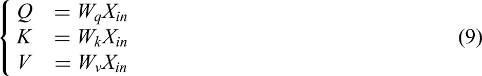
In previous studies, researchers used the original sequence as input, making the encoding process use sequences with high complexity and strong randomness as inputs. The ICEEMDAN algorithm is used to reduce component noise, enhance the physical meaning of components, and effectively process non-stationary data sequences. As shown in Figure 2, we will use the decomposed multivariate IMF as the input of the Encoder, with a shape of
Transformer prediction model and integrated energy system (IES) data shape.
The calculated multi-head self-attention is feed forward and decoded through multivariate feedforward layers and residual operations in the Decoder. Obtain the final output through the final linear layer. Finally, repeat this operation until all IMFs are predicted. Reconstruct each component to obtain the final predicted results.
We name the hybrid model proposed in this article ICEEMDAN-MIC-Transformer and use a multivariate load energy dataset as input to predict future regional short-term loads. The main steps of this model are as follows:
step 1 (Sequence decomposition)
The preprocessed multivariate energy load dataset is decomposed into sub sequences of IMFs from high frequency to low frequency using the ICEEMDAN algorithm.
step 2 (Correlation analysis)
The decomposed IMF subsequences were subjected to correlation analysis by the MIC algorithm.
step 3 (Sequence recombination)
Reconstruct sequences with high similarity, where multivariate loads are used as inputs to the encoder of the prediction model, and single loads are used as inputs to the decoder.
step 4 (Training and forecasting)
Divide the dataset into training, validation, and testing sets in proportion, and obtain the results for each component.
step 5 (Result synthesis)
Sum up all the predicted sequences to obtain the final IES load result.
Data analysis and index description
The IES load dataset comes from the campus metabolic system, which is an interactive web tool (Arizona State University, n.d.). Through this system, it is possible to view the consumption of regional level IES loads in Arizona State University (ASU) in real-time. This includes the residential load of students and faculty, the load of administrative, teaching and experimental buildings, and the load of parking buildings. These loads include electric load, cold load, and heat load. There is a central factory in ASU, which has several natural gas burning burners to supply hot water to various buildings in the Temple campus. In addition, the central factory of ASU has large coolers for cooling the water supplied to buildings. It is worth mentioning that the heat energy value in the IES load data is calculated based on the decrease in temperature and flow rate of hot water entering and exiting the building. The cold energy value is calculated based on the increase in temperature and flow rate of water entering and exiting the building.
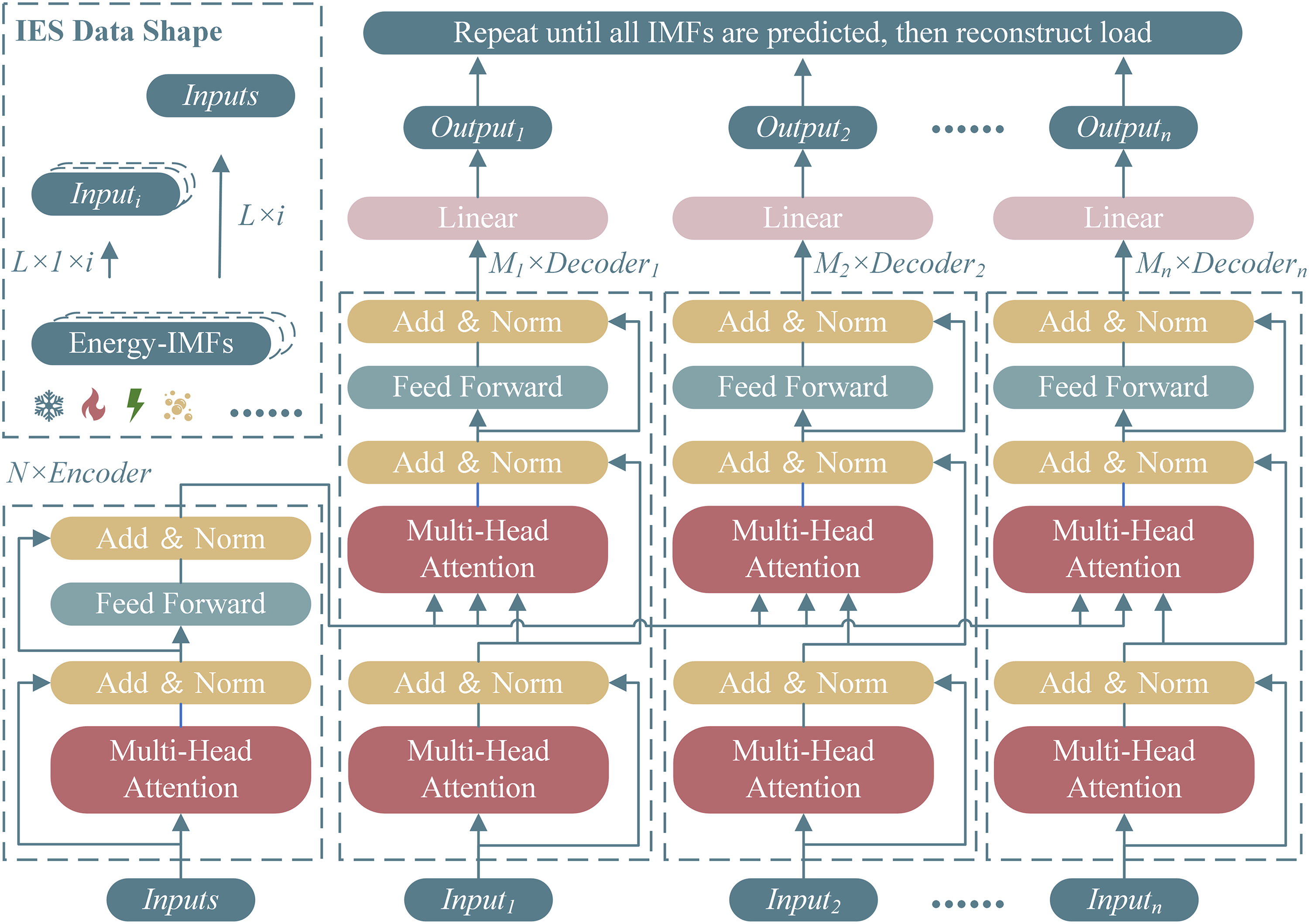
In the process of collecting IES load data, it is inevitable to encounter problems such as data loss and anomalies, which can lead to distortion of the IES load dataset. The distorted IES load dataset will inevitably have a negative impact on the load forecasting results. Therefore, the IES load dataset must undergo data preprocessing before entering the load forecasting model, including missing value filling, outlier handling, visualization analysis, stationarity analysis, and feature construction. The Preprocessing process of multivariate load data is shown in Figure 3.
Preprocessing process of multivariate load data.
Outlier handling refers to identifying and removing outliers in load data that deviate significantly from the normal range. Common methods include
Data analysis
The dataset contains three-year IES load data with hourly granularity. Therefore, the length of the dataset is
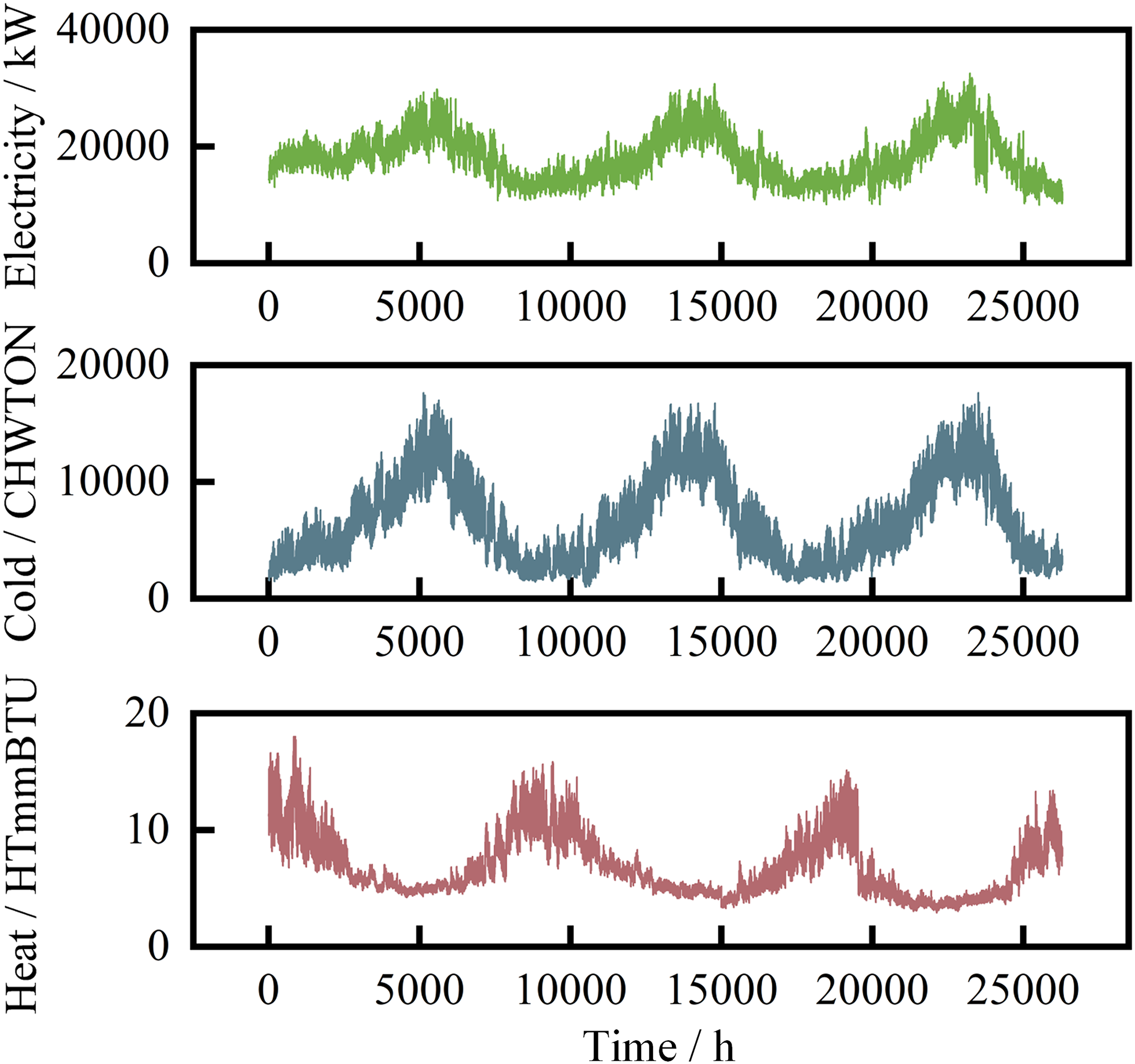
Integrated energy system (IES) load series of Arizona State University in the United States.
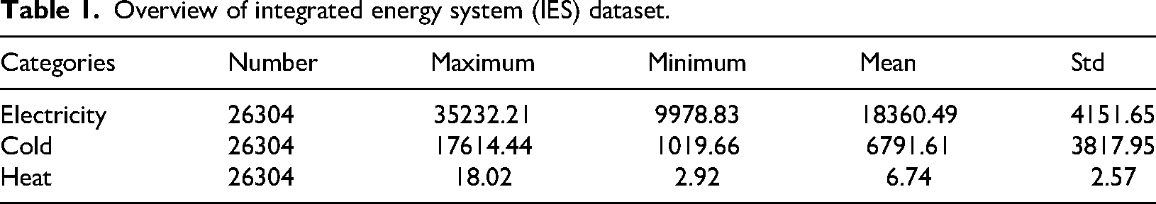
Overview of integrated energy system (IES) dataset.
From the preprocessed multivariate energy load data, it can be seen that the trend of cold load is similar to that of electricity load, while the trend is exactly opposite to that of heat load. This is in line with the load characteristics of regional level IES.
In fact, most load forecasting models add relevant physical information to the dataset, such as temperature, humidity, and geographic climate, in addition to the target load sequence. However, through our testing, we found that the physical information mentioned above does not significantly improve the predictive performance of the model proposed in this paper, but it can lead to a significant increase in the computational power requirements of the model. Therefore, following the principle of Occam’s Razor, we choose not to use datasets containing physical information and instead opt for datasets containing only multivariate loads.
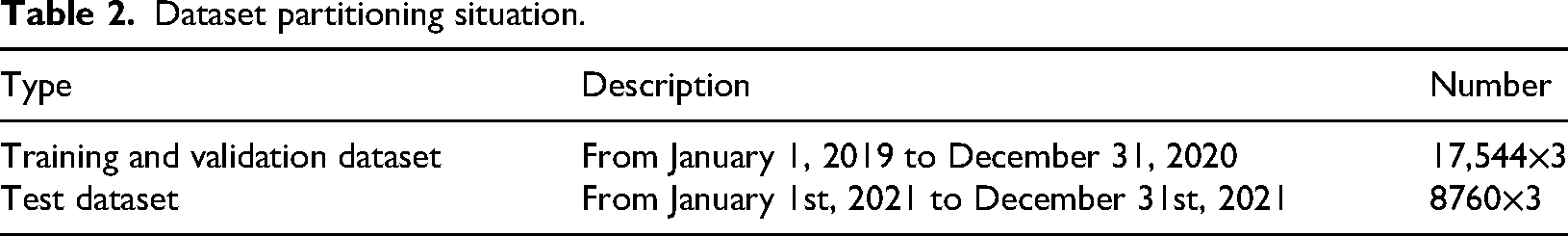
The dataset used in this article is a 1-hour granularity dataset, covering a three-year period from January 1, 2019 to December 31, 2021. We selected 17544 time points from January 1, 2019 to December 31, 2020 as the training and validation sets, and the entire year of 2021 as the testing set, as shown in Table 2.
Dataset partitioning situation.
Load decomposition and correlation analysis
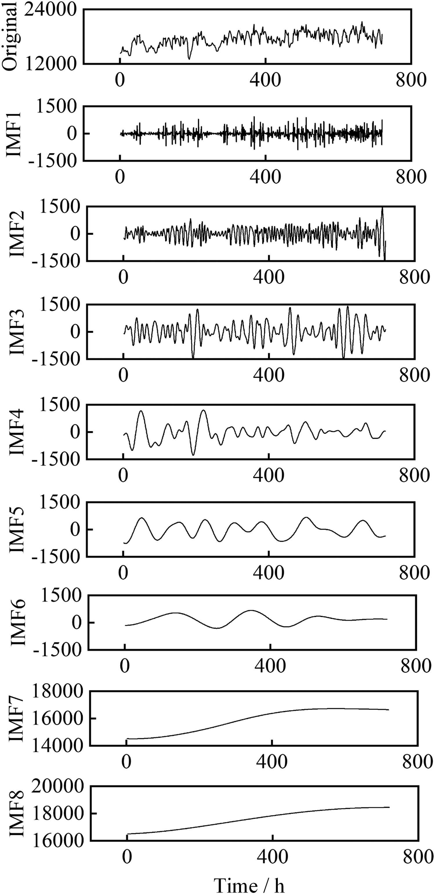
Due to the gradual progress in load forecasting, the first month’s electricity load is decomposed first, and the decomposition results are shown in Figure 5. The length of this sequence is
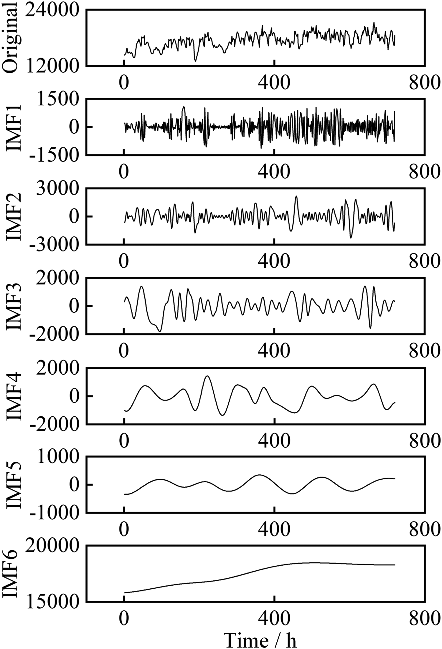
Partial electric load sequence after improved complete ensemble empirical mode decomposition with adaptive noise (ICEEMDAN) decomposition.
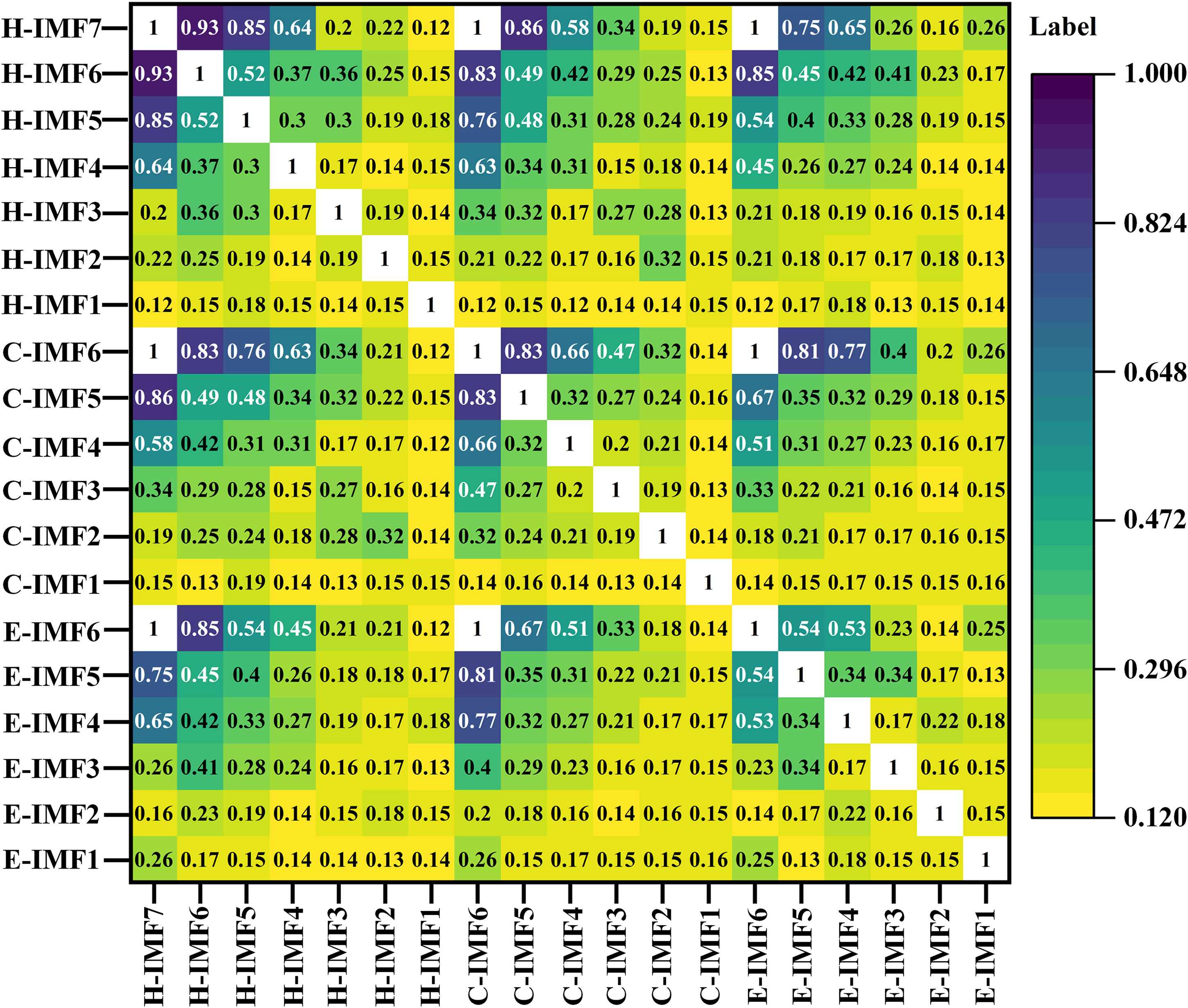
The ICEEMDAN algorithm adaptively decomposes the original signal into six IMFs, with frequencies decreasing sequentially. The first five IMFs have different physical meanings. The last IMF represents the overall trend, representing an upward trend in regional electricity load during the first month. Then, the cold load signal and the heat load signal are separately decomposed by the ICEEMDAN algorithm to obtain their respective IMFs. Perform correlation analysis on each component using MIC, and the resulting heatmap is shown in Figure 6.
IES load heatmap under MIC correlation analysis. MIC: maximum information coefficient; IES: integrated energy system.
From the heat map, it can be seen that the correlation between the trend components of a single load is 1, which means that multivariate loads exhibit strong correlation in the trend. The correlation between IMF components with lower frequencies and their respective trend components is relatively high, generally greater than 0.8. As the frequency increases, the correlation rapidly decreases. There is almost no correlation between the highest frequency IMF components.
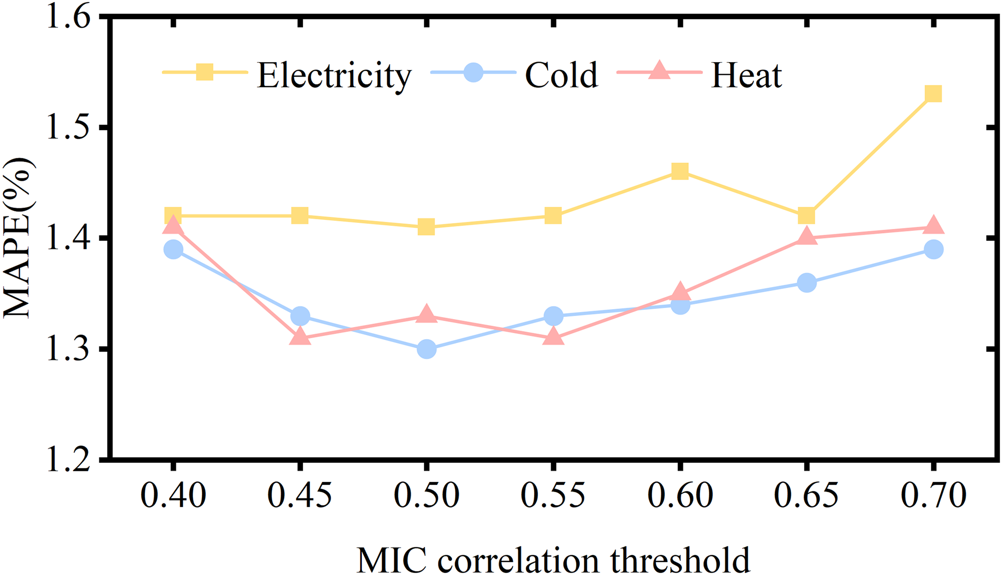
The selection of screening threshold for MIC is a problem worthy of in-depth research. We have consulted a large amount of literature, and generally setting the threshold of MIC between 0.5 and 0.6 is considered reasonable. In order to improve the readability of this article and the credibility of threshold settings, we changed the MIC screening threshold and used the model proposed in this article for single step prediction. We obtained the prediction results of the multivariate factor load forecasting model under different thresholds, as shown in Figure 7.
Maximum information coefficient (MIC) threshold search.
From the Figure 7, it can be seen that the electric load and cold load have optimal results when the MIC threshold is 0.5, while the heat load has optimal results when the MIC threshold is 0.45 and 0.55. The predicted results of the three loads almost all decrease when the MIC threshold decreases or increases. In summary, it is reasonable to set the MIC threshold of 0.5 for the multivariate load forecasting model. Therefore, we reconstructed these IMF components into trend components, high-frequency components (with scores greater than or equal to 0.5), and low-frequency components (with components below 0.5).
To further demonstrate the applicability of ICEEMDAN in IES multivariate load forecasting, we added two types of decomposition algorithms, EEMD and CEEMDAN, and conducted two experiments on reconstruction error and modal aliasing. Due to limited space in the main text, the decomposition results of EEMD and CEEMDAN can be found in Figure 13 and Figure 14 in the Appendix.
Firstly, we reconstruct all the IMFs obtained by the three decomposition algorithms. By comparing with the original signal, it can be concluded that only the reconstructed EEMD signal has occasional errors of the order of
Then, we perform modal aliasing analysis on all IMF components obtained from the three decomposition algorithms to determine whether all IMF components are in the same frequency band. The analysis results are shown in Table 3.
Decomposition algorithms and their IMF components with modal aliasing Analysis.
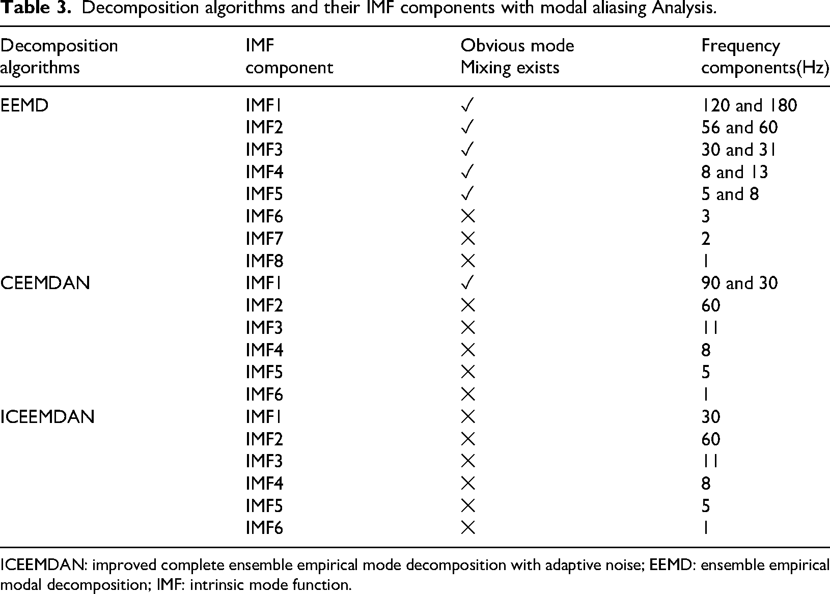
ICEEMDAN: improved complete ensemble empirical mode decomposition with adaptive noise; EEMD: ensemble empirical modal decomposition; IMF: intrinsic mode function.
From Table 3, it can be seen that there is a significant mode mixing phenomenon in some IMF components of EEMD and CEEMDAN. The modal aliasing phenomenon in EEMD is quite severe, with at least two frequency components present in IMF1 to IMF5. And all IMF components of ICEEMDAN detected obvious mode mixing phenomenon, that is, all IMF components are in independent frequency bands. In summary, the ICEEMDAN algorithm has a good separation effect on the original signal, can better characterize multivariate information, and has better applicability to IES multivariate load data.
To further quantify the improvement of separability by MIC grouping, we calculated the signal-to-noise ratio (SNR) after MIC grouping. Calculate the SNR by using the portion of IMF with MIC scores higher than the set threshold as the signal, and the portion of IMF with MIC scores lower than the set threshold as the noise. The formula for calculating SNR is as follows:
In the formula,
From the SNR results, it can be seen that the original signal contains a large amount of noise. For example, when reconstructing the IMF7 of heat load and the IMF6 of cold load through the MIC algorithm, the SNR values of the original electric load, cold load, and heat load are 25.41, 11.65, and 16.37 dB, respectively. When reconstructing the IMF5 of electric load through the MIC algorithm, the SNR values of the original electric load, cold load, and heat load are 23.98, 11.18, and 15.19 dB, respectively. The calculation process and results of other data are similar to the above, all below 30 dB. Obviously, the SNR values mentioned above are far below the threshold requirements of normal signals, indicating that signal filtering through the MIC algorithm is very necessary.
In addition to calculating the SNR value, we also quantified the improvement in separability of MIC grouping by comparing the MI values before and after reconstruction. According to the formula (7), the MI values between the IMF7 of heat load and the electric load, cold load, and heat load before and after reconstruction are 4.94 bits and 5.02 bits, 4.87 bits and 5.02 bits, 4.23 bits and 4.98 bits, respectively; The MI values between the IMF6 of cold load and the electric load, cold load, and heat load before and after reconstruction are divided into 3.88 bits and 6.38 bits, 6.04 bits and 6.38 bits, and 4.03 bits and 5.61 bits. The calculation process and results of other data are similar to those mentioned above. Obviously, the MI value between the reconstructed signal filtered by MIC and the predicted target signal has been improved to a certain extent, which means that the correlation between the two signals is stronger and theoretically can improve the predictive performance of the prediction model to a certain extent.
Evaluating index
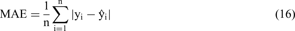
To verify the predictive performance of the model proposed in this paper, mean absolute percentage error (MAPE) was used to measures the error. This evaluation index measures the relationship between predicted results and actual loads. In both horizontal comparison experiments and vertical ablation experiments, predictive models with lower MAPE achieved higher results evaluation of predictive performance. In order to present the predictive results of the model to readers in multivariate dimensions, we have also added three evaluation metrics: Root mean square error (RMSE), mean absolute error (MAE), and mean absolute scaled error (MASE).
For load forecasting values 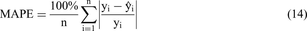

Result analysis
Configuration and forecast results
All experiments in the paper were conducted by a computer in the same configuration. In terms of hardware, the CPU is Intel Core i5-12490F 3.00 GHz, the GPU is NVIDIA GeForce RTX 4060Ti, and the memory is 16 GB. In the software part, we have chosen version 3.8 of Python. And deep learning models were selected from Python 1.1.1 and Tensorflow 2.4.1.
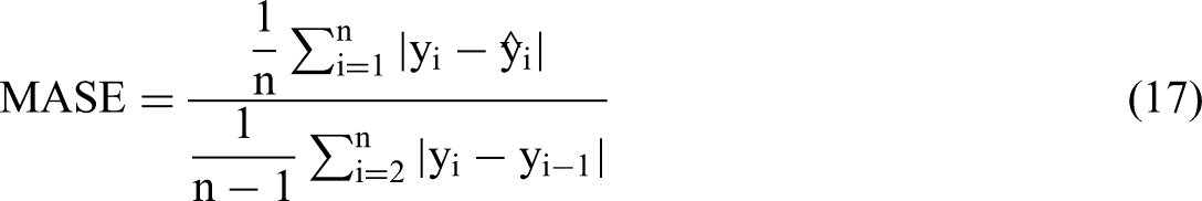
In order to ensure that the current hyperparameters of the studied model are optimal in the calculation example, the grid search method is used to optimize the hyperparameters. The optimization objectives, scope, and optimal parameters are shown in Table 4.
Model hyperparameters optimization.
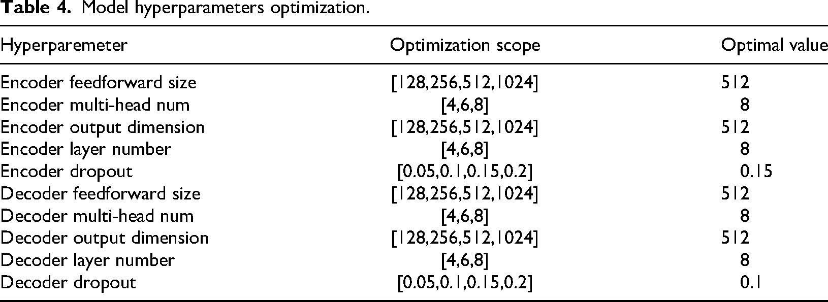
According to different prediction requirements, the sliding window length and prediction step size of the prediction model should also be changed accordingly. As shown in Figure 8, for an energy load sequence with a granularity of hours, if the sliding window length is set to 96 and the prediction step size is set to 1, it means that in each iteration of the model, the 4-day data from the historical energy load sequence is used to predict the trend of energy load for the next hour.
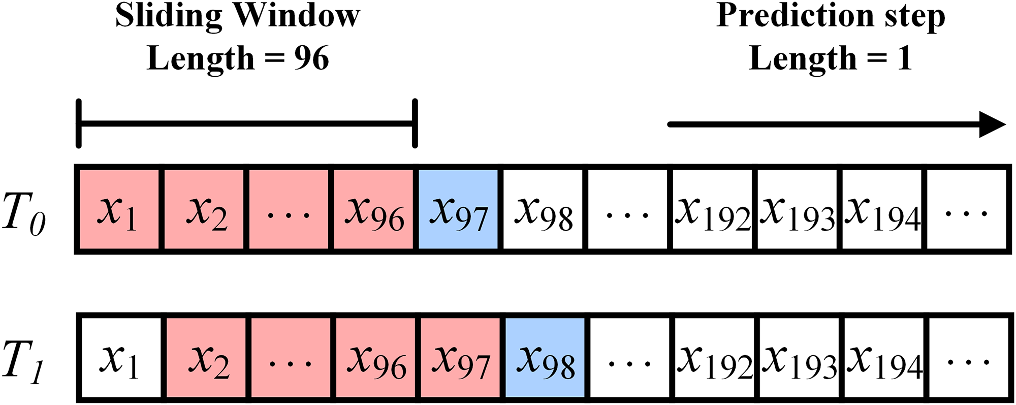
Schematic diagram of sliding prediction window.
The model training cycle is 200 epochs. If the real-time MAPE is not lower than the current optimal MAPE within 10 epochs, it will stop early.
The model and its ablation model (Transformer type deep learning model) proposed in this article are optimized using grid search algorithm, while the other deep learning models and machine learning models are optimized using particle swarm optimization algorithm. Under the model parameters shown in Table 5, use the model studied in this paper to perform load forecasting on the ASU comprehensive energy system dataset group. Use the proposed model to perform mean reconstruction on the predicted results of electricity load, cold load, and heat load, respectively. The prediction results are shown in Figure 9.
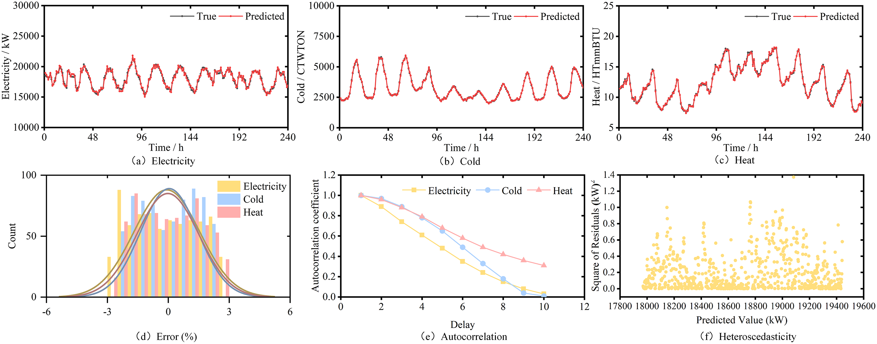
The prediction results of the proposed model.
Optimization of hyperparameters in comparative models.
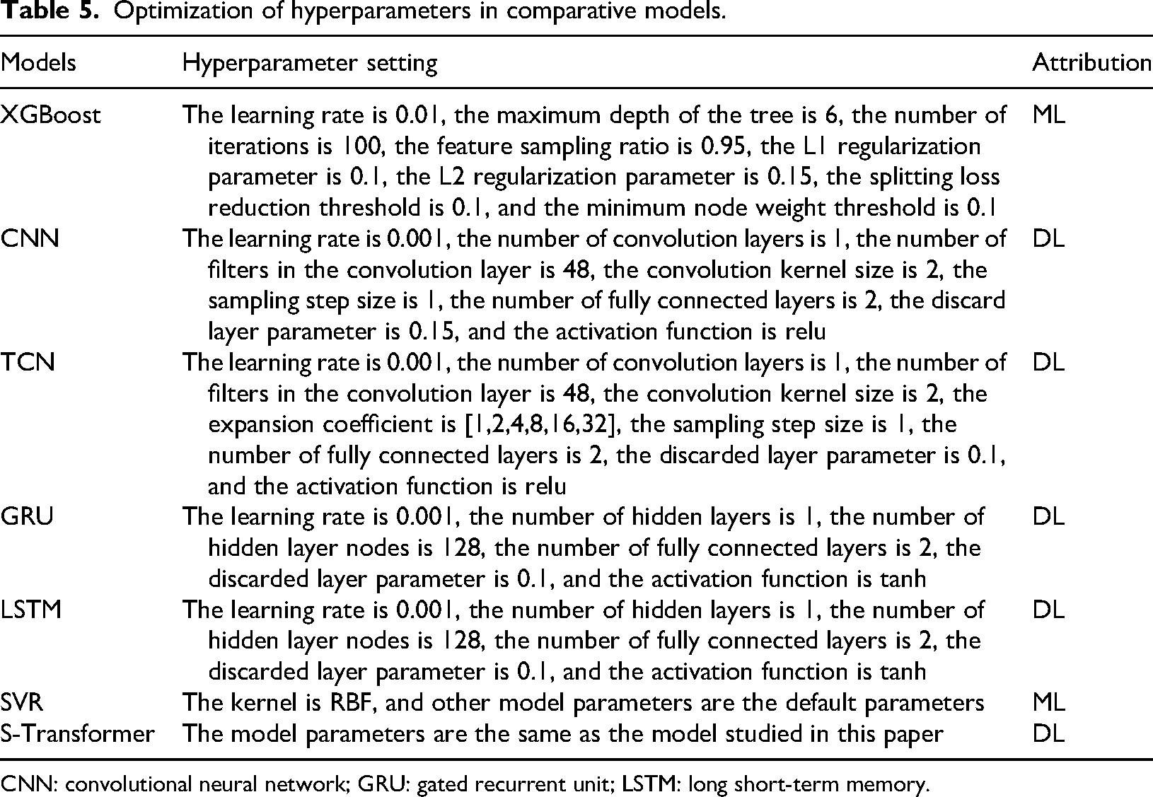
CNN: convolutional neural network; GRU: gated recurrent unit; LSTM: long short-term memory.
From the Figure 9(a)(b)(c), it can be seen that when the prediction step size is 1, the reconstructed predicted value curve fits well with the true value curve, with only a small error appearing at the corner. This indicates that the model studied in this paper has high predictive performance for multivariate load forecasting tasks, and can to some extent explore the hidden regularity information in the original energy data, which has certain engineering application value.
In addition, in order to further explore the predictive performance of the studied model on real datasets, this paper also conducts normal distribution statistical analysis on the errors, as shown in Figure 9(d). It can be seen that the prediction error of electricity load is relatively concentrated, while the prediction error of cold load and heat load is relatively dispersed. However, the normal distribution of the three is expected to be around zero. Therefore, when using deep learning models for load prediction, the prediction error is expected to not deviate from the reasonable range of zero, which is convenient for IES energy suppliers to make reasonable scheduling arrangements.
In order to further analyze the prediction results, we conducted residual diagnosis on the multivariate load forecasting results, including autocorrelation test and heteroscedasticity test.
Firstly, we conducted an autocorrelation test on the results of multivariate load forecasting. Autocorrelation refers to whether there is a statistical dependency between observed values of the same variable at different time points, as shown in Figure 9(e).
From the Figure 9(e), it can be seen that the autocorrelation of heat load is the best, followed by cold load and electric load. This is related to users’ energy consumption habits, as heating and cold loads are more affected by climate factors. When the climate changes periodically with the seasons, the energy consumption of heating and cold loads also exhibits periodic changes. On the other hand, users’ electricity consumption lacks regularity and is less affected by climate factors, resulting in a smaller autoregressive coefficient.
Then, we tested the heteroscedasticity of the prediction model. Heteroscedasticity refers to the phenomenon in which the variance of random error terms in a regression model changes with changes in explanatory variables or observations. The heteroscedasticity test was conducted on the results of multivariate load forecasting using Breusch-Pagan (BP) test. Figure 9(f) shows the BP test results of electric load, with a statistical value of 0.9231 and a p-value of 0.3367. Through calculation, the BP test statistics and
Through multiple repeated experiments, we obtained the final experimental results and used the mean as the main evaluation metric for the predictive performance of the prediction model. In addition, the mean, maximum, minimum, quarter, half, and three-quarters values of the results of electric load, cold load, and heat load on the training and validation sets are shown in Figure 10.
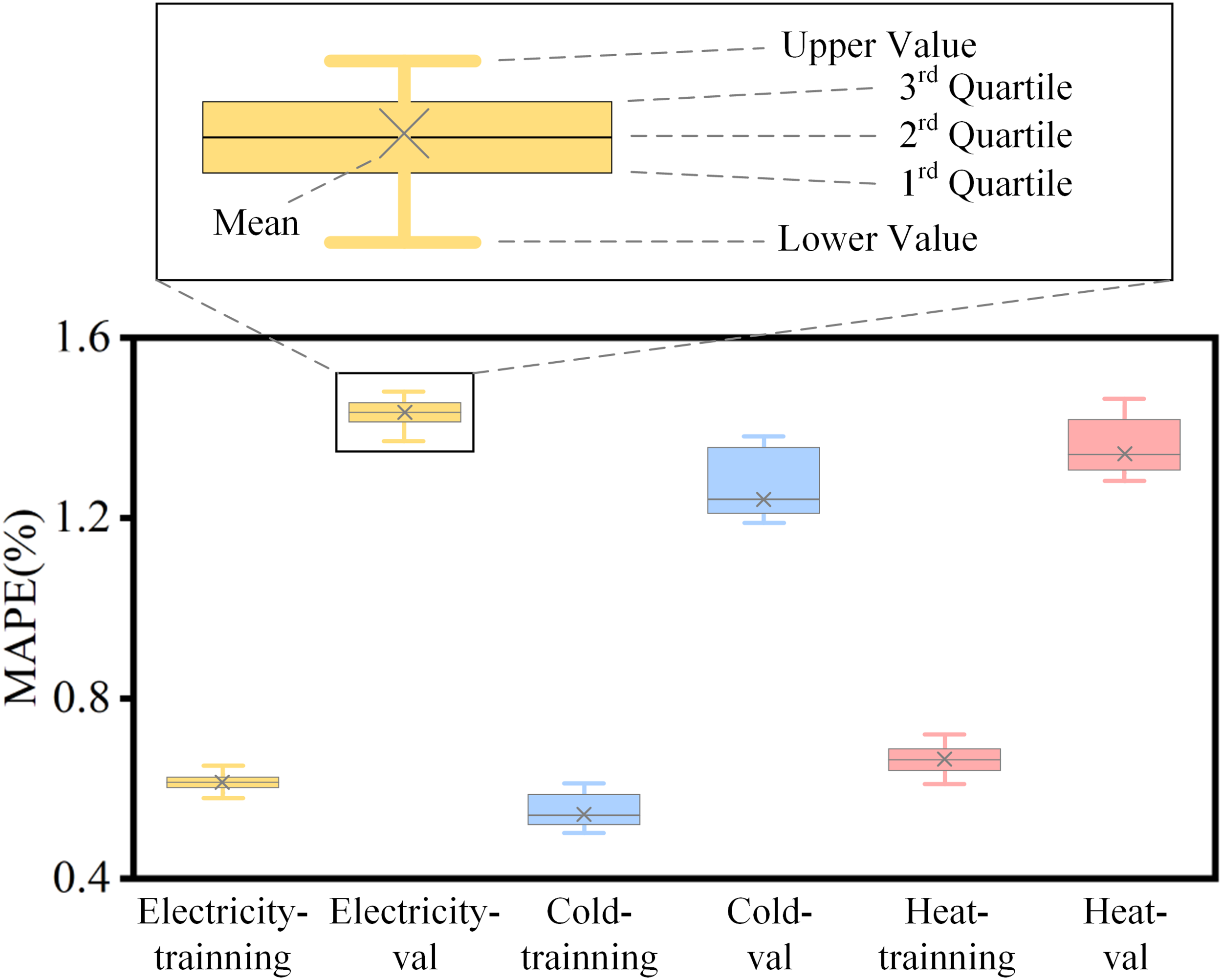
The comparison of the proposed model with training set and validation set.
Horizontal comparison experiment
In order to verify the superiority of the model studied in this paper compared with other algorithm models, this paper selects the depth learning model which is widely used and has better performance, as well as the classical machine learning model as the benchmark model for simulation experiments. It is worth mentioning that many literatures show that the hybrid deep learning model has better prediction performance than the single deep learning model in most cases. To sum up, the benchmark model selected in this paper includes the following two parts:
Classic machine learning models that only contain a single algorithm: LSTM, GRU, CNN, TCN, XGBoost, SVR and S-Transformer (Transformer model for single load forecasting, with single sequence input and single sequence output). Because this kind of algorithm can establish new types of models (such as stacked LSTM and Bi-LSTM models) through stacking and bidirectional forms, which will affect the prediction results, only single-layer unidirectional model is used for simulation experiments. The hybrid deep learning model including feature extraction module: CNN-LSTM, CNN-GRU, TCN-LSTM and TCN-GRU. This kind of algorithm first uses convolution model to extract the features of the original sequence, captures the sequence information through multidimensional mapping, and finally uses deep learning model for load forecasting.
In order to verify the superiority of the model compared with the traditional machine learning model and the hybrid deep learning model which only contains a single algorithm, this paper uses the ASU IES data set to carry out a horizontal comparative experiment on the benchmark model previously studied. It is worth mentioning that, in order to ensure the reliability of the horizontal comparison experiment, this paper selects the same environmental parameter settings for the simulation experiment.
Under the hyperparameter settings shown in Table 5, the comparative experimental results of the model studied in this paper and various single benchmark models under the optimal hyperparameter and different prediction step sizes are shown in Figure 11 and Table 6. For the sake of simplicity in the article, MAPE will be used as the main evaluation metric in the future. The results using RMSE, MAE, and MASE as evaluation indicators can be found in Tables 10, 11, and 12 in the Appendix.
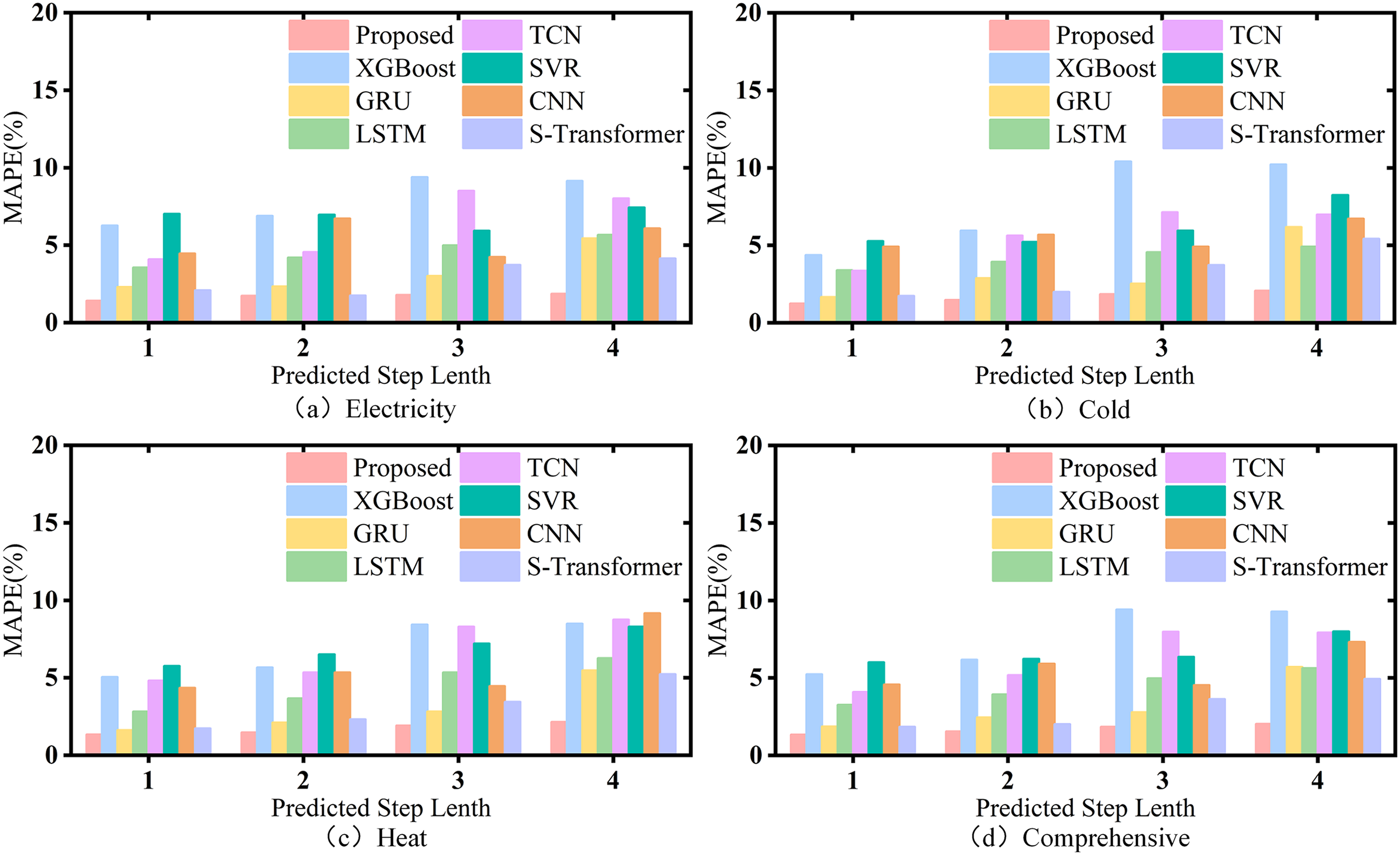
Comparison of experimental results with single models.
Comparison of experimental results with single Models.
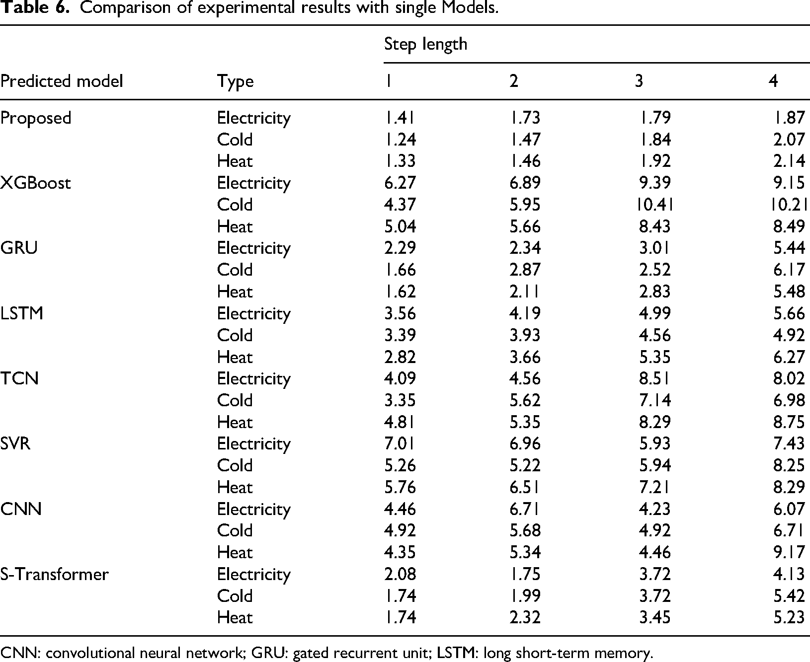
CNN: convolutional neural network; GRU: gated recurrent unit; LSTM: long short-term memory.
For a single model, the model studied in this paper achieves the optimal results in the case of asynchronous length, and the reconstructed load curve fits the original curve most closely. In addition, many algorithmic models, such as XGBoost and CNN, grow faster in the process of increasing the step size, indicating that predictive stability of the model is poor. However, the MAPE of the model studied grows slowly in the process of step size growth, so it has high predictive stability and can meet different prediction requirements in engineering applications.
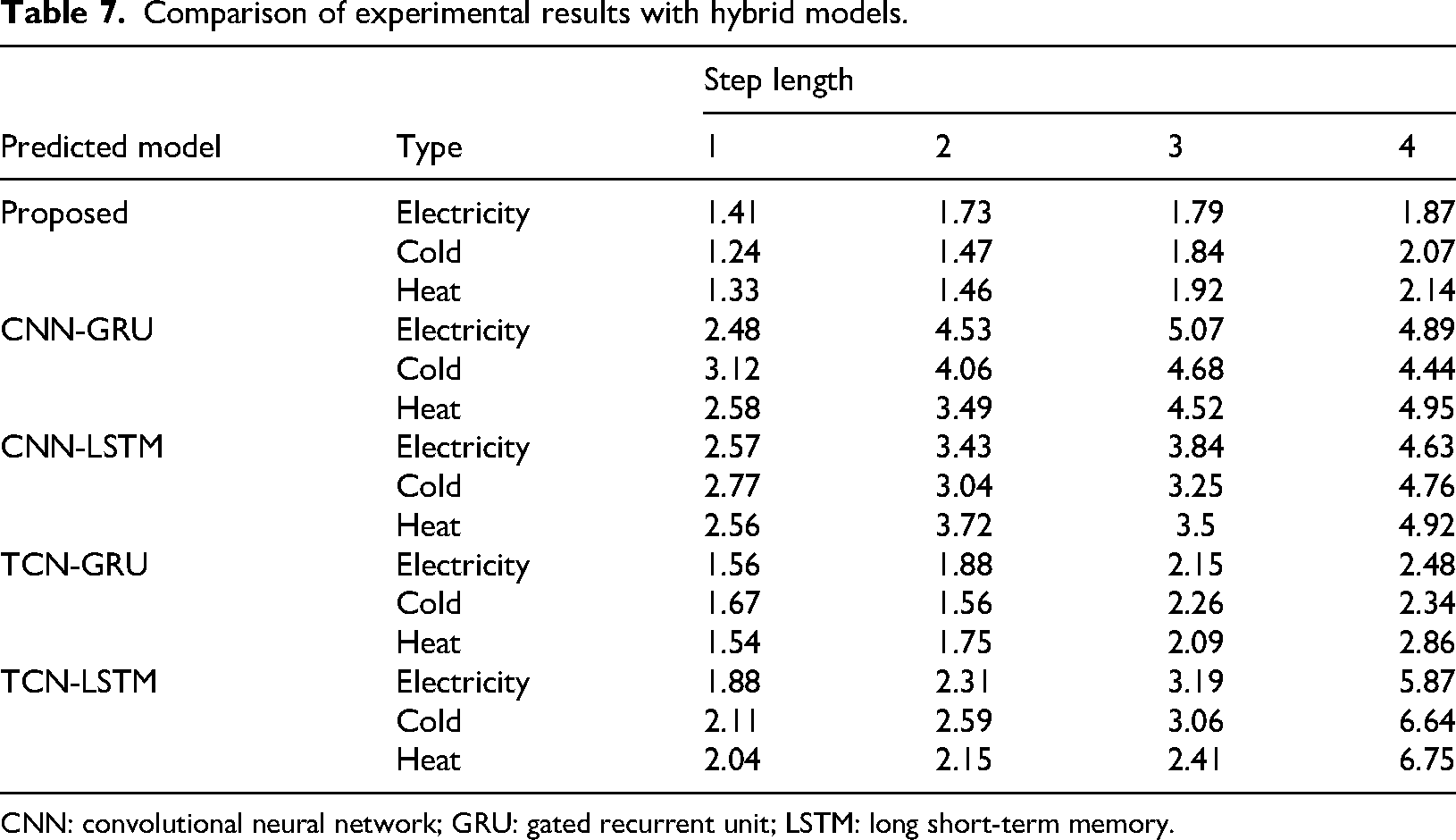
In addition, the comparative experimental results of the studied model and each hybrid benchmark model under optimal parameters and different prediction steps are shown in Figure 12 and Table 7. It is worth mentioning that, due to the large amplitude difference of electric load, cold load and heat load, the superposition of multivariate loads using the mean value will lead to the weight of electric load and cold load is too heavy, which is obviously unreasonable. Therefore, the total load selected here is the mean value of the multivariate load forecasting results, that is, all load types are in the same weight.
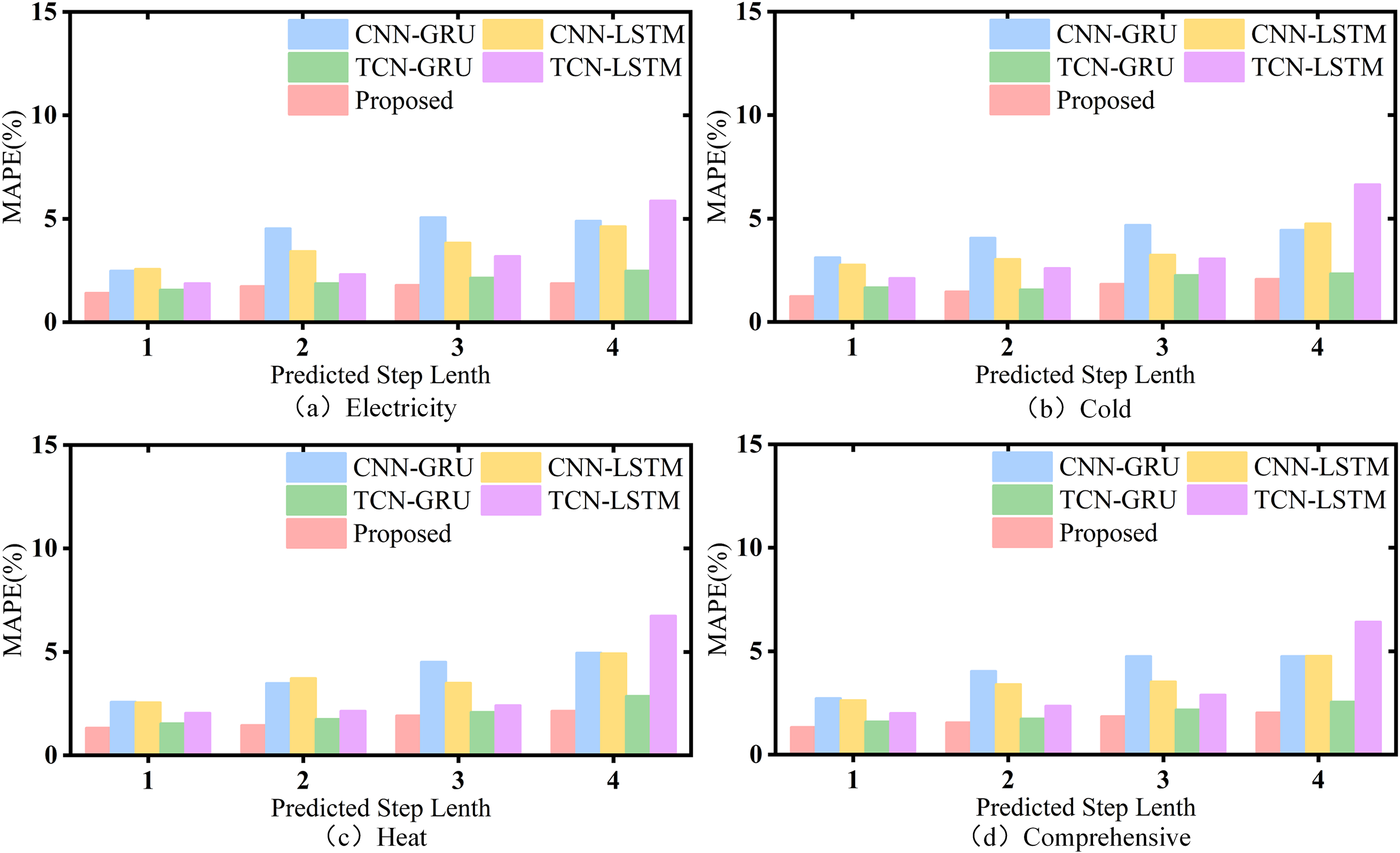
Comparison of experimental results with hybrid models.
Partial electric load sequence after ensemble empirical mode decomposition (EEMD) decomposition.
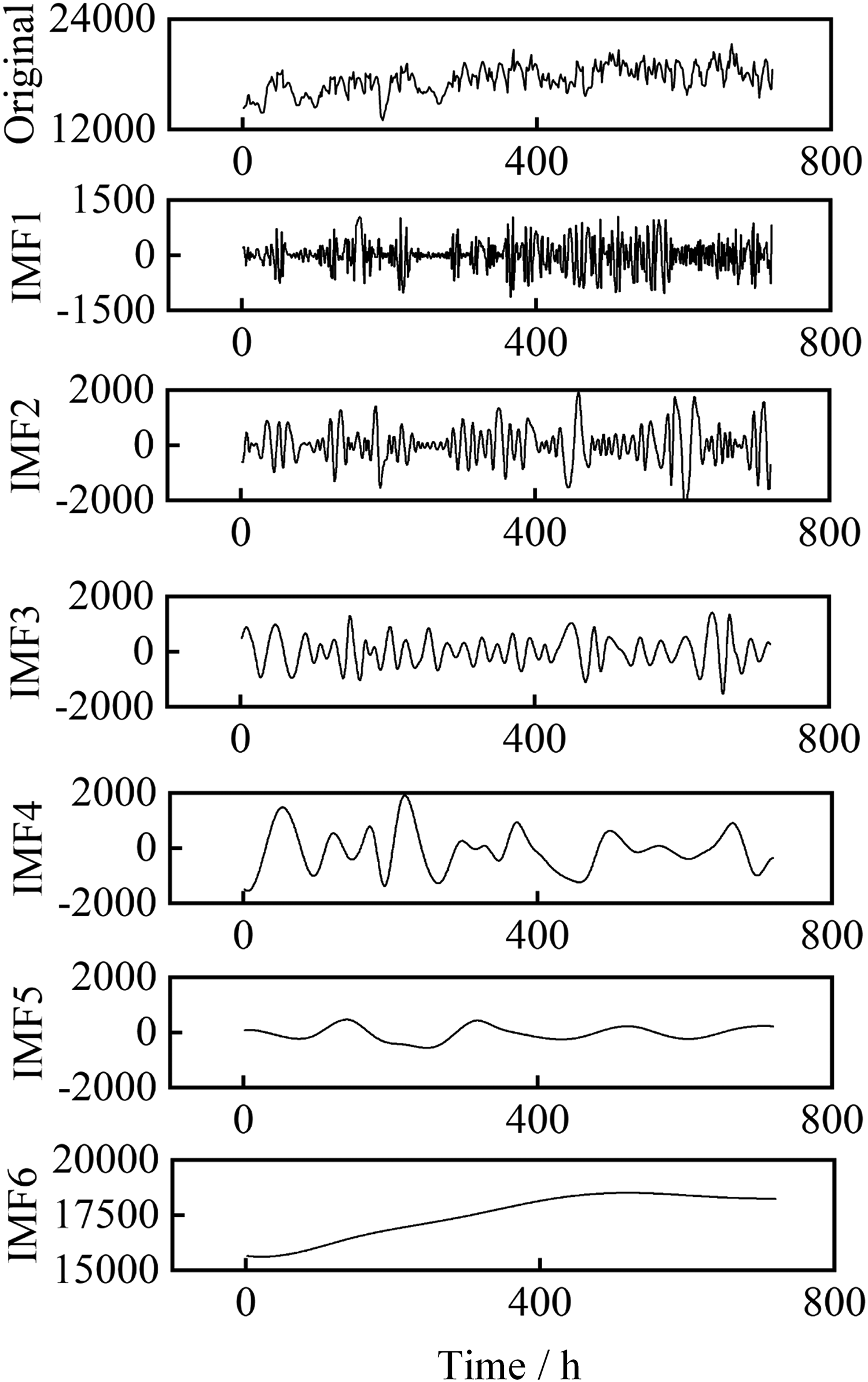
Partial electric load sequence after complete ensemble empirical mode decomposition with adaptive noise (CEEMDAN) decomposition.
Comparison of experimental results with hybrid models.
CNN: convolutional neural network; GRU: gated recurrent unit; LSTM: long short-term memory.
It can be seen from Figure 12 and Table 7 that for the hybrid model, the model studied in this paper also achieved the optimal results at different prediction steps, indicating that compared with the traditional method of extracting the original sequence information using convolution model, this model can effectively extract and utilize the original sequence feature information using the parameter matrix with high complexity of hidden layer. Therefore, compared with the hybrid benchmark model, the model studied in this paper also has performance advantages.
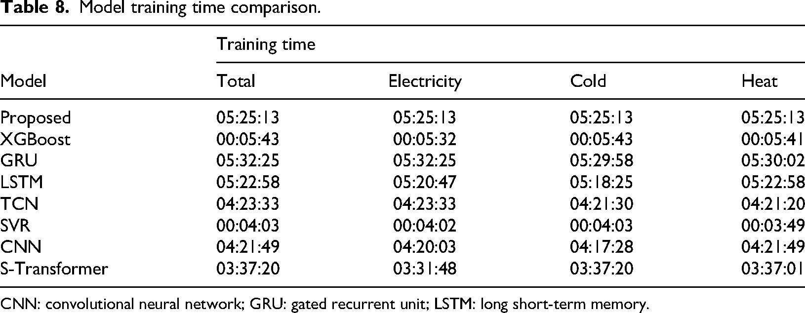
In order to better represent the training cost of our model, we measured the training/inference cost of all compared models. The training/inference cost is the total duration from the start to the end of the model training, as shown in Table 8. It is worth mentioning that only the multivariate Transformer class prediction models can output results at the same time, while other prediction models have a sequence of multivariate load output times (such as the heat load being calculated first, and the electric load and cold load being calculated later). Therefore, the training/inference cost is based on the calculation time of the last type of load.
Model training time comparison.
CNN: convolutional neural network; GRU: gated recurrent unit; LSTM: long short-term memory.
To further evaluate the significance of the performance of the model proposed in this article, we conducted a significance test using the Diebold Mariano (DM) method. The DM test evaluates significance by comparing the difference sequences of prediction errors between two models. Firstly, make assumptions about the DM test:
Null hypothesis
Alternative hypothesis
By comparing the prediction sequences of the model proposed in this article with those of other models and conducting DM significance tests, all results showed
In order to ensure that data information is not leaked, we conducted a controlled experiment using a method of randomly dividing the training set and validation set for electricity load prediction. The MAPE of the validation set reached 0.82%, which is a significant improvement compared to the MAPE of 1.41% in the formal experiment, indicating a significant improvement in prediction performance. The above experiment proves that there was no data leakage in the test set of the formal experiment.
Longitudinal ablation experiment
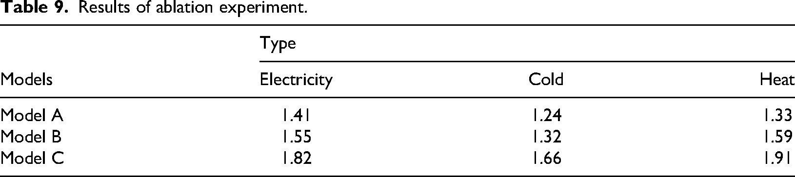
In order to verify the superiority of the model studied in this paper compared with the naive model and ablation model, longitudinal ablation was performed on the model studied in this paper. Ablation experiment is to explore the changes of part of the model compared with the overall performance, that is, remove a part of the model each time, and check whether the prediction performance of the model is reduced, so as to test the reliability of each module in the model. The experimental model after ablation includes the following parts:
Model A
The model proposed in this paper.
Model B
The original IES data set is directly input into the model without decomposition by CEEMDAN algorithm.
Model C
After ceemdan decomposition, IMF components are not used for correlation analysis by MIC algorithm.
The results of ablation experiment is shown in Table 9. From the ablation experiment, it can be seen that Model A has the best predictive performance among the three types of loads.Model B and Model C have lower prediction accuracy to some extent than the proposed model, therefore the various sub modules of the model are feasible.
Results of ablation experiment.
Comparison of experimental results with single models (RMSE).
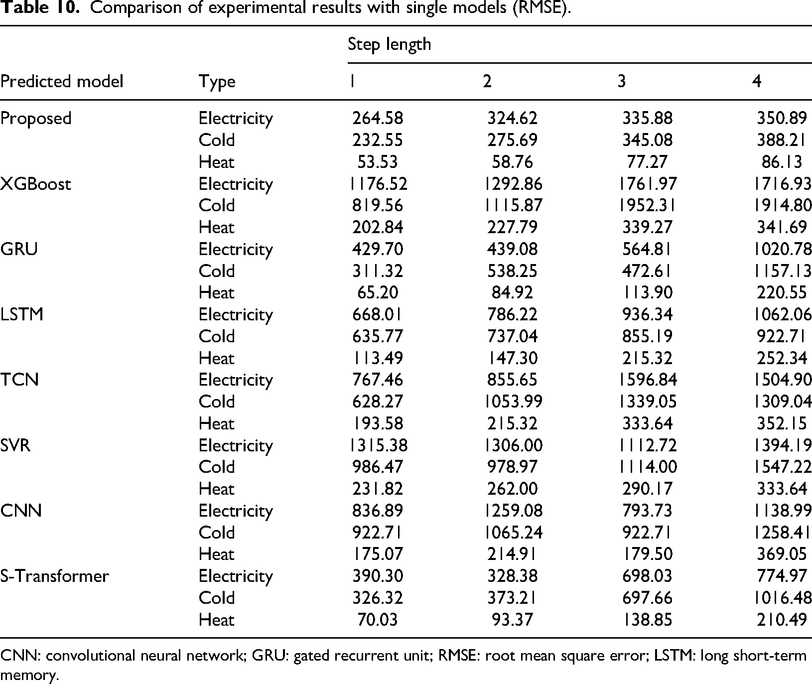
CNN: convolutional neural network; GRU: gated recurrent unit; RMSE: root mean square error; LSTM: long short-term memory.
Comparison of experimental results with single models (MAE).
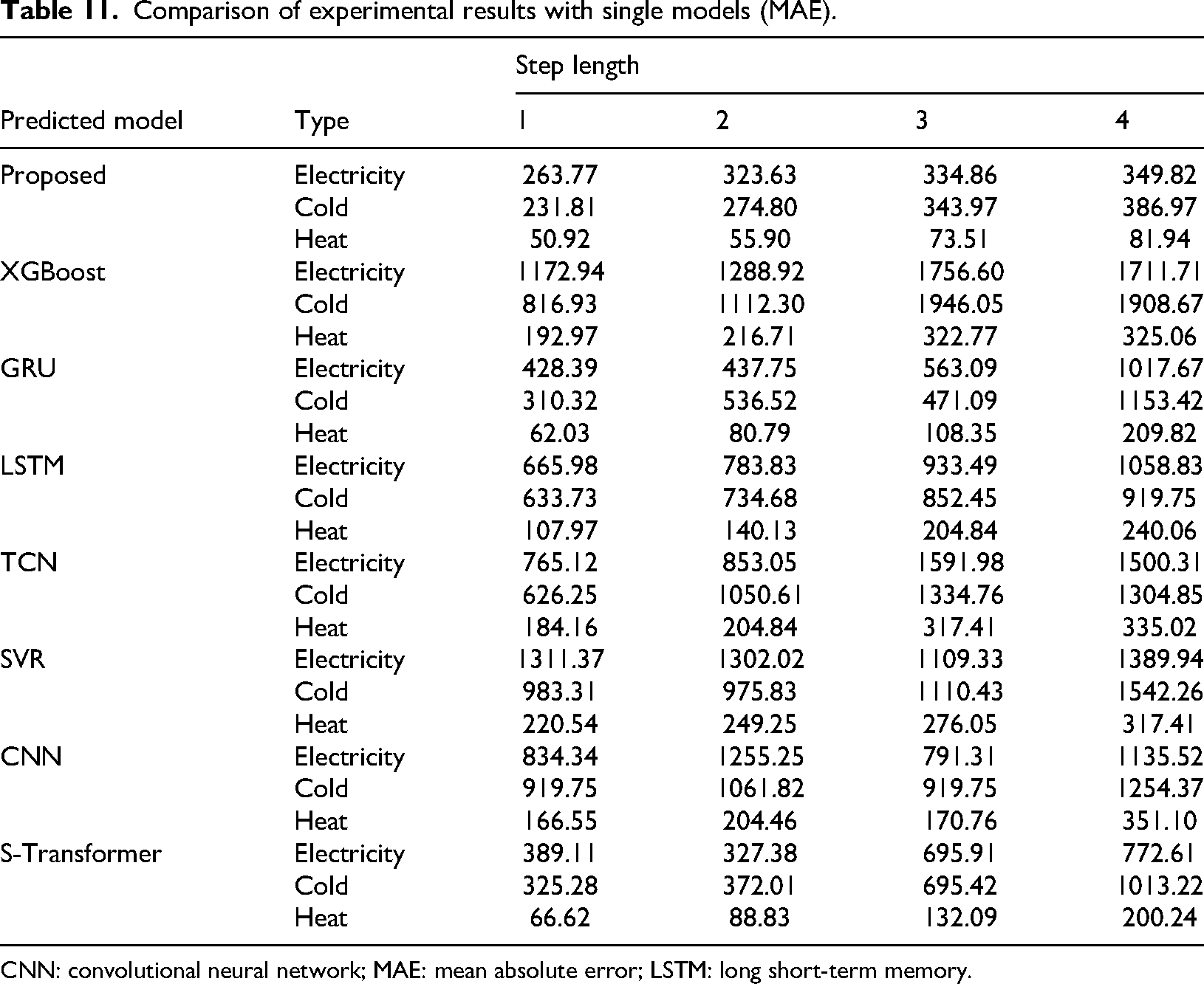
CNN: convolutional neural network; MAE: mean absolute error; LSTM: long short-term memory.
Comparison of experimental results with single models (MASE).
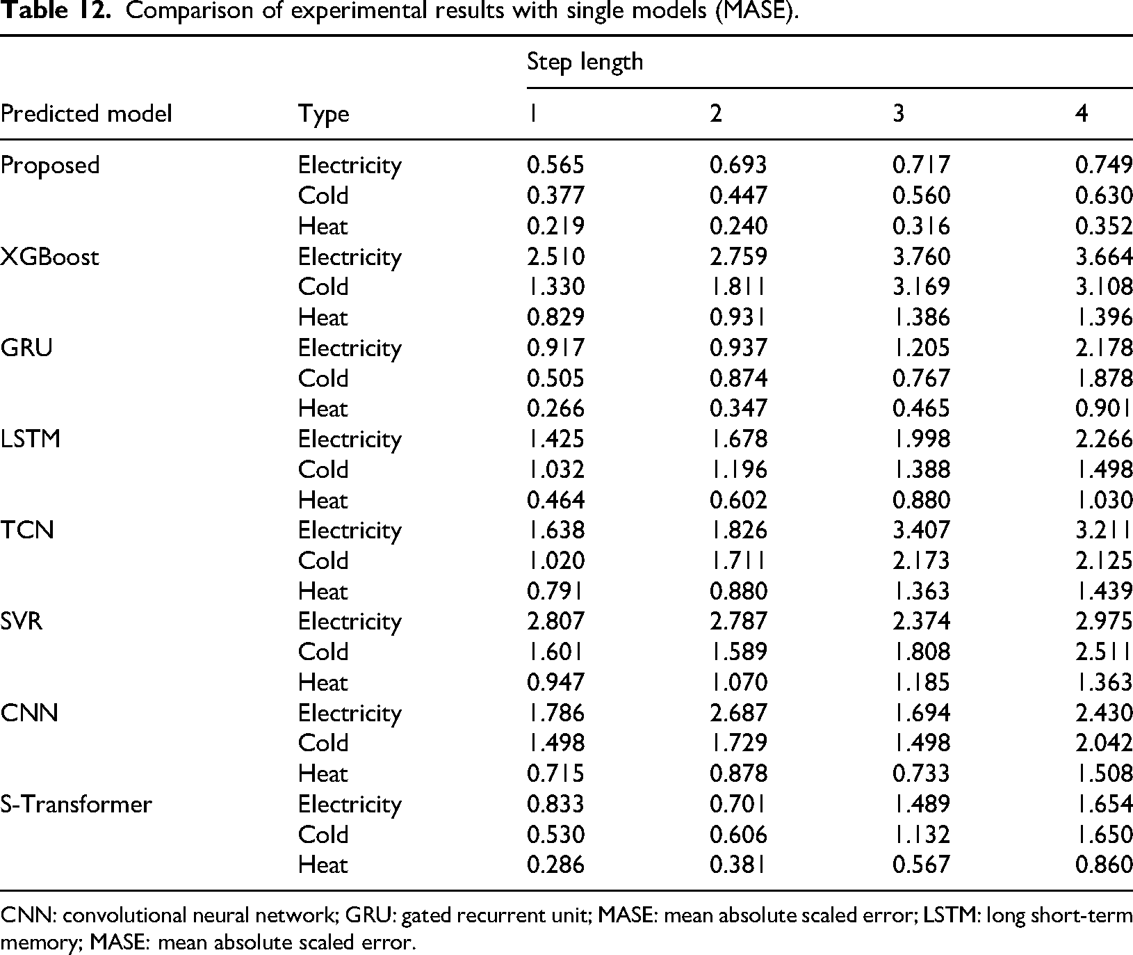
CNN: convolutional neural network; GRU: gated recurrent unit; MASE: mean absolute scaled error; LSTM: long short-term memory; MASE: mean absolute scaled error.
Conclusion
A short-term prediction model based on ICEEMDAN-MIC-Transformer is proposed for IES load time series with high coupling correlation. This method utilizes a Transformer model based on self attention mechanism to better capture dependency relationships in long-term data information. The ICEEMDAN decomposition algorithm was introduced into IES, which clearly captured the detailed changes in the time series and extracted internal information. In addition, introducing MIC for correlation analysis of various time series and reconstructing several IMF components after classification. The reconstructed multivariate dataset and a single dataset are used as inputs to the Transformer model for forecasting, resulting in short-term load forecasting results. The prediction results indicate that the model can accurately predict the IES load. Compared to traditional machine learning and deep learning methods, the model has better predictive performance in the horizontal comparison experiment. The longitudinal ablation experiment shows that each module of the model is feasible, and the predictive performance of the model after ablation has decreased compared to the original model. In summary, this model has certain research significance and application value for load forecasting research under IES.
Footnotes
Funding
The authors received the following financial support for the research, authorship, and/or publication of this article: This work was supported by the Science and Technology Research Program of Chongqing Municipal Education Commission (Grant No.KJZD-K202302602), the Science and Technology Research Program of Chongqing Municipal Education Commission (Grant No.KJQN202402604), the Science and Technology Research Program of Chongqing Municipal Education Commission (Grant No.KJQN202302604), the Science and Technology Research Program of Chongqing Electric Power College (Grant No.D-KY202516).
Declaration of conflicting interests
The authors declared no potential conflicts of interest with respect to the research, authorship, and/or publication of this article.