
Abstract
To effectively utilize a feature set to further improve fault diagnosis of a rolling bearing vibration signal, a method based on multi-fractal detrended fluctuation analysis (MF-DFA) and smooth intrinsic time-scale decomposition (SITD) was proposed. The vibration signal was decomposed into several proper rotation components by applying this new SITD method to overcome noise effects, preserve the effective signal, and improve the signal-to-noise ratio. Wavelet analysis was embedded in iteration procedures of intrinsic time-scale decomposition (ITD). For better results, an adaptive threshold function was used for signal recovery from noisy proper rotation components in the wavelet domain. Additionally, MF-DFA was used to reveal the multi-fractality present in the instantaneous amplitude of the proper rotation components. Finally, linear local tangent space alignment was applied for feature dimension reduction and to obtain fault characteristics of different types, further improving identification accuracy. The performance of the proposed method is determined to be superior to that of the ITD-MF-DFA method.
Keywords
Introduction
Because of complex operating environmental and objective factors, rolling bearing failures frequently occur in industrial processes. Safety insurance in production, improved quality, and the overall economic benefits of the product are very critical issues of modern industrial processes. A good solution to these problems is the application of effective performance monitoring and fault diagnosis processes.
Feature extraction characterizes the running state of rolling bearings and, thus, is one of the key research methods of rolling bearing fault diagnosis. According to the analysis of the vibration mechanism, the functional model corresponding to the classification of fault severity was established. 1 The non-linear and non-stationary characteristics of the signal and the interference of external factors on the obtained vibration signal are all factors that affect the extraction of features from complex vibration signals.2-5
For this purpose, a large number of articles on feature extraction methods can be found in the literature. As a classical time–frequency analysis method, wavelet transform (WT) is applied to mechanical fault diagnosis for its multi-scale analysis features, high time–frequency resolution, and rigorous mathematical foundation. Lou and Loparo used WT to process accelerometer signals,6 in which the standard deviation of wavelet coefficients was used to generate eigenvectors. Then, a neural fuzzy reasoning system was used as a classifier for bearing fault diagnosis. Liu and Ling proposed a fault diagnosis method based on wavelet packet theory.7 The coefficients were taken as the pattern features of a ball-bearing fault, which greatly improved the effectiveness of pattern recognition. An improved Hilbert-Huang transform method based on WT was presented by Peng et al.,8 which overcame the inevitable defects of the two methods when used separately for rolling bearing fault detection. Researchers have achieved much progress in fault detection and diagnosis methods based on WT.9-12 With the purpose of improving the adaptability of wavelet applications, an adaptive threshold function is presented in this study, which was used to improve the efficiency of the denoising procedure. Because of the addition of shape adjustment factor m, the function becomes a comprehensive threshold function.
Recently, researchers have proposed an improved matching pursuit algorithm which has greater diagnosis precision in rolling bearing fault diagnosis.13 New adaptive time–frequency analysis methods have been developed and have become a topic of concern in this field, namely, the empirical mode decomposition (EMD) and intrinsic time-scale decomposition (ITD).14 An et al. proposed a fault diagnosis method based on ITD to determine the fault types of the wind turbine bearing. 15 In this case, the frequency center of the main proper rotation component was regarded as the fault feature vector. Yu and Liu applied a sparse coding shrinkage method based on ITD to fault diagnose for rolling bearings and effectively extracted the impulse component of the bearing vibration signal. 16 The ITD method is superior to the EMD method in reducing invalid components and mode mixing, 14 and the calculation time of the ITD method is much lesser than that of the EMD method, which significantly improves the work efficiency in practical applications. Nevertheless, its disadvantages should not be ignored, the ITD method is based on the linear transformation of signals to extract the baseline signal, which may lead to distortion, the production of burr, and end effects. To solve this drawback, many schemes have been proposed.17,18 Hu et al. proposed a new approach named ensemble intrinsic time-scale decomposition (EITD) to deal with end effects and avoid distortion. 19 The steps included using cubic spline interpolation to fit baseline control points and mirror extension.
However, these improved ITD methods cannot meet the requirement of fault diagnosis perfectly. First, these methods use predictive models to improve classical ITD methods by spreading each single side of the signal, while a signal expansion method, such as that used with images, is imperfect in eliminating boundary distortion. In addition, prediction errors will occur during the screening process and destroy all proper rotation components (PRCs). Second, the mechanical fault signal in the initial period tends to exhibit a low signal-to-noise ratio (SNR) and small amplitude, and the traditional ITD method based on signal expansion is verified by analyzing the pure signal, whereby the weak signal with low SNR is not considered. Third, the portion of the signal that is extended by experience cannot reflect the true characteristics of the original weak signal. To solve the problem of noise interference and improving SNR, a method combining ITD and WT is proposed in this study. A correlation coefficient is used in the sifting process to show the iterative error and correlation relationship.
The fractal features hidden in the signal reflect the dynamic mechanism of the non-linear system under different states. Based on multi-fractal detrended fluctuation analysis (MF-DFA), a number of fault diagnoses and detection methods have been developed.20–22 In this study, MF-DFA is applied to reveal the intrinsic multi-fractality in every extracted PRC. Finally, linear local tangent space alignment (LLTSA) 23 is implemented to reduce the value of dimension of the features, which will improve the accuracy of diagnosis.
In this paper, the concepts of ITD and MF-DFA are reviewed, and an adaptive threshold function is shown. The proposed methods of eliminating noise and restraining the end effects are discussed in detail, and a comparison of the proposed method and the original ITD method is shown. Moreover, rolling bearing signal decomposition based on smooth intrinsic time-scale decomposition (SITD) is studied, while MF-DFA and LLTSA are utilized to obtain the feature vector.
Description of ITD method and MF-DFA method
The ITD method, a new self-adaptive signal decomposition method, is especially useful to analysis non-stationary or non-linear signals. MF-DFA is able to eliminate trend interference effectively and represent the intrinsic multi-fractal property. In this study, MF-DFA is applied to reveal the intrinsic multi-fractality in every extracted PRC.
The ITD data decomposition method
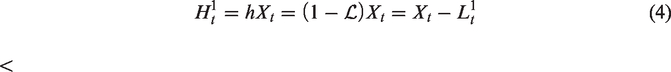
The ITD method decomposes any non-stationary vibration complex signal Xt into a series of PRCs with practical physical meaning and a monotonous trend signal.
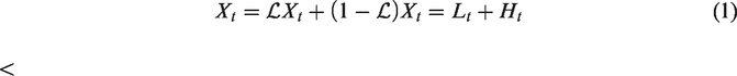
Suppose
It is assumed that Xt is available on
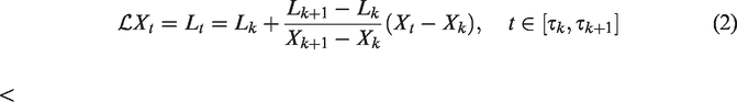
For signal Xt, the baseline-extracting operation is performed, and the first baseline signal,
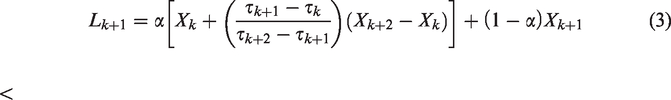
The baseline signal is set as the input signal when it is not a monotonic function. The above process is repeated P times until a drab trend signal is obtained. More precisely
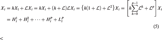
The ITD method represents a significant advancement in EMD, because the linear interpolation operation and selection process in EMD decomposition are eliminated. It improves upon the conventional method of EMD in terms of efficiency and accuracy, completing in a single step what the EMD may require numerous iterations to achieve. Instantaneous amplitude and frequency of PRC reflect the time–frequency information of the contaminated signals in real time.
The components decomposed by the ITD method have a certain physical significance. They are suitable for analyzing signals containing Amplitude Modulation-Frequency Modulation components, because the characteristics of the original signal are well reflected. Therefore, it is more suitable for vibration signal feature extraction and fault diagnosis of bearings and gearboxes.
MF-DFA—A method for eliminating trends
It overcomes the deficiencies of DFA which must be used for stationary time series.
The MF-DFA procedure is shown in detail:
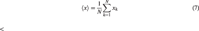
Assume that xk is a time series with a length of N, and “profile” is defined as
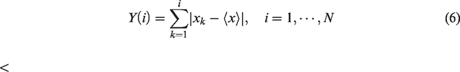
The profile Y(i) is divided into 2. The local trend for every segment is fitted by applying the least-squares algorithm. Then, the mean square error is calculated, which is determined as
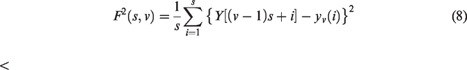
for the v-th segment, v = 1,…, Ns and
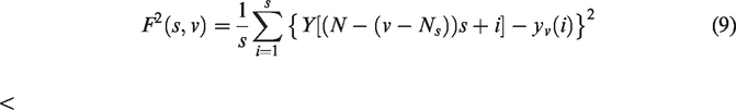
In the v-th segment, yv(i) is the fitting polynomial. Linear, quadratic, cubic, or higher order polynomials are employed in the fitting procedure (defined as DFA1, DFA2, DFA3, or etc., respectively).
Different orders of DFA may yield different detrended results that show the different abilities of eliminating trends in the series.
3. Define the q-th order fluctuation function by calculating the average of all segments
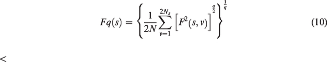
when q = 2, the procedure is the same as the standard DFA.
For different timescales s, repeat steps 2–3 to get the Fq(s). Thus, by implementing the fitting polynomial of each segment, the trend of that segment will be eliminated efficiently.
4. Analyze log–log plots Fq(s) versus s for each value of q so as to determine the scaling behavior of the fluctuation functions Fq(s). If the series xi is long-range power-law correlated, Fq(s) and s are related as follows
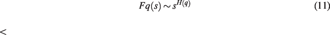
H(q) is defined as the generalized Hurst exponent and may be related to q. Normally, H(q) is used to describe the impact of past time series on current and future ones because of its ability of long-range correlation. For rolling bearings, owing to external factors, the status may change from normal to fault status. However, the fault status will persist all the time for its self-irreparability. Therefore, the variable corresponding to Hurst exponent under different statuses can distinguish between normal status and fault status with high performance for vibration fault diagnosis.
In nature, multi-fractals exist in common circumstances. Oppositely, mono-fractals are rare. Therefore, the multi-fractal analysis is generally applicable to reveal intrinsic fractal characteristics. However, noise interference problems will influence the MF-DFA method. The proposed method shown herein effectively overcomes this problem.
SITD method
With the purpose of effectively using the sensitive features contained in feature set for fault diagnosis and overcoming the noise interference problem, a new SITD decomposition method based on ITD was proposed.
Although the ITD approach has many advantages, we cannot ignore its problems, such as signal distortion, end effects, and redundant PRCs. These problems will influence feature extraction. One of the causes of these problems is the algorithm itself, while another cause is noise interference. As we all know, the fault vibration signal includes the resonant component, the impulse signal produced by the faulty bearing and noise. Impulse signals and noise are high-frequency signals, and their noise affects the extraction of fault signals. Therefore, noise elimination is the key step in feature extraction. For the purpose of eliminating the noise signal, the SITD method was proposed, in which wavelet analysis was embedded in the iteration procedures of ITD, which could preserve the effective signal and improve the SNR. To get better results, an adaptive threshold function was analyzed in the wavelet domain.
An adaptive threshold function
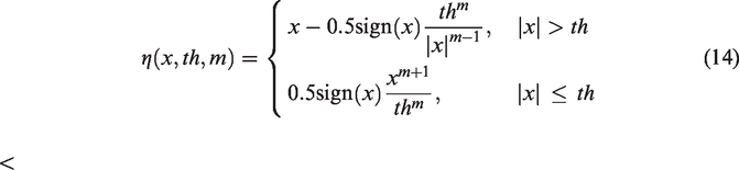
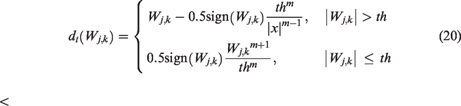
To maintain the effective signal details as much as possible in the denoising process, a threshold function that is superior to both hard and soft threshold functions was designed. The proposed threshold function is presented as follows
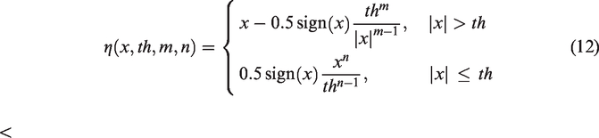
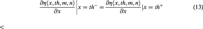
Meanwhile, n = m + 1; therefore, the expression of the threshold function (12) after adding the first-order derivable property is
When m is transformed, zone 1 and zone 2 from Figure 1(b) can be represented as shown enlarged in Figure 1(c) and (d). When m = 1, the curve of the function and the soft threshold function in Figure 1(a) almost coincide. When m > 10, the curve is very close to the hard threshold function. The threshold function could nullify, shrink, or maintain the wavelet coefficients in different regions, unlike the soft and hard threshold functions. The region that could shrink the wavelet coefficient is the critical region in which the WT coefficient is composed of signal and noise. To achieve the purpose of maximally retaining the details of the signal while removing noise, a more realistic initial signal for target recognition is needed. The size of the contraction region could be adjusted, and the removal ratio of the noise signal could be controlled, resulting in the retention ratio of the signal details.
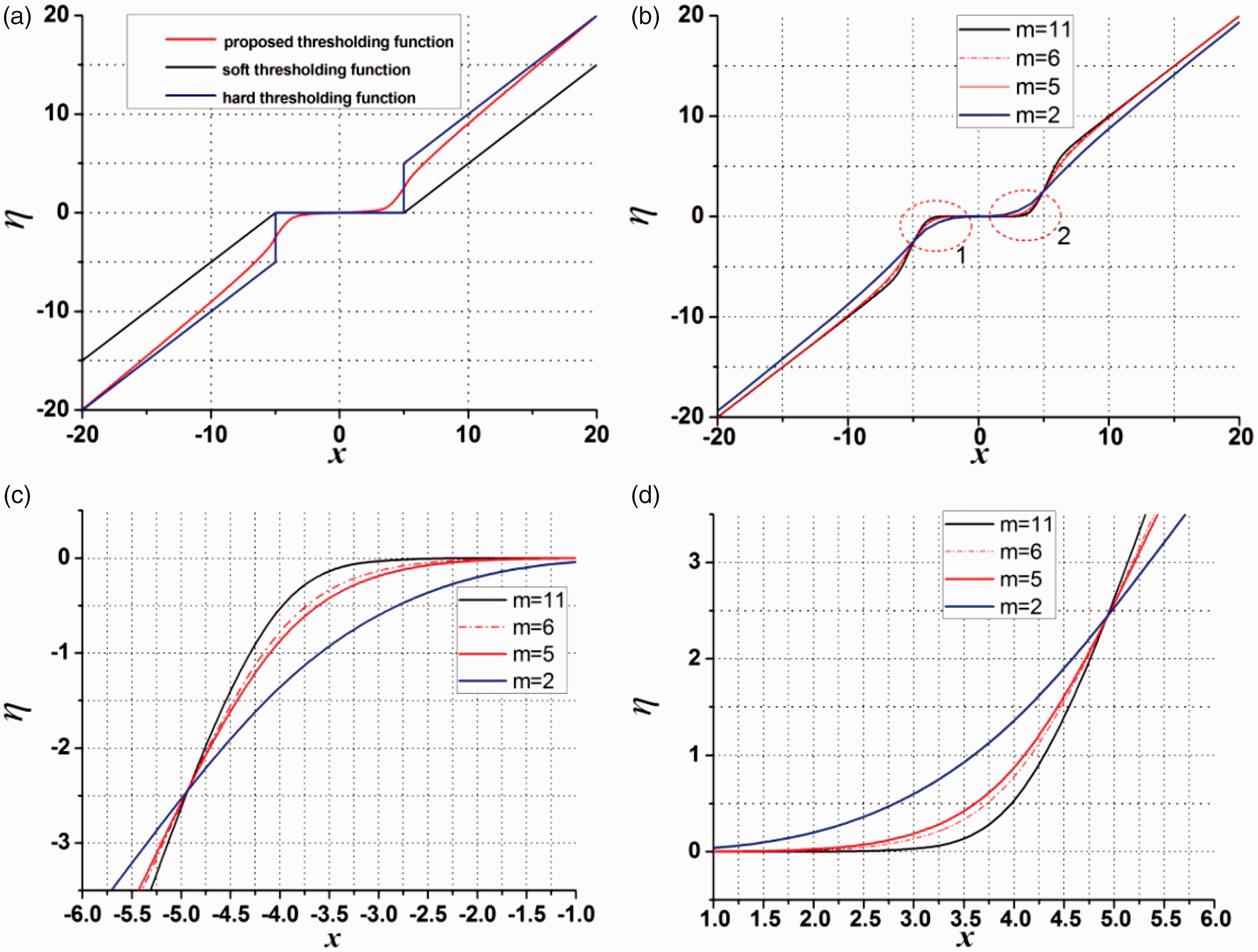
Proposed threshold function with different m values. (a) Proposed threshold function. (b) Proposed threshold function with hard and soft threshold function different m value. (c) Region one. (d) Region two.
In conclusion, the threshold function could achieve a smooth transition of wavelet coefficient attenuation in the critical region. The size of the critical region was determined by adjusting the parameter m. The higher m is, the more similar the process is to the process of the hard threshold function. Simultaneously, the wavelet coefficient in the critical area could be contracted on a large scale. Therefore, when the value of m is relatively large, it is suitable to process a noisy signal with a low SNR. Conversely, the smaller the value of m is, the more wavelet coefficients are in the critical region, in which the wavelet coefficients with signal detail could be better preserved in the case of shrinking noise factor, thereby maintaining the original local singularity of the signal.
To more effectively preserve the signal singularity in the signal denoising process, the threshold function η(x, th, m) applicable to wavelet coefficients at different scales could be selected by adjusting the parameter m in equation (14). The corresponding denoising strategy is as follows: use the partial hard threshold function to denoise for the coefficient on a small scale, eliminating most of the noise; use the partial soft threshold function to denoise for the coefficient on a large scale and realize coefficient contraction in the critical area. For adaptive selection of the threshold function for specific signals, the mathematical model is established as follows
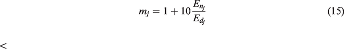
The selection of suitable wavelet parameters is indispensable for signal analysis. The adaptive threshold function is used to improve the denoising efficiency and provide a more real input signal for the subsequent target recognition process. Considering the applicability of the function, a comprehensive threshold function is generated by adding shape tuning factor m.
Smooth intrinsic time-scale decomposition
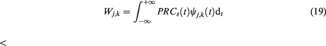
The flow chart of the proposed wavelet-analysis-embedded ITD method is shown in Figure 2, while the transformation of PRCs into wavelet domain is performed through the equation as follows

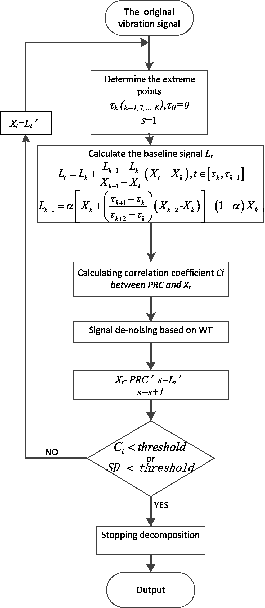
Flow chart of SITD. WT: wavelet transform; SD: standard deviation; PRC: proper rotation component.
Here,
The evaluation function is described as follows

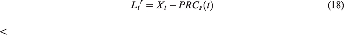
Unlike previously, the new purified PRC0 is subtracted from the original signal to obtain a new baseline signal, which is set as the input signal.
Repeating the above-mentioned process is necessary in every sifting stage until a final monotonic trend is achieved.
The operation procedures of SITD are as follows:
Compute the PRCs based on the procedure discussed previously. Calculate the wavelet coefficients by the following equation
Estimate the new denoised wavelet coefficients by presetting a positive value for threshold th
Reconstruct PRCs from the denoised coefficients and approximate the coefficients by using the inverse WT. Subtract the new PRCs from Xt and obtain the residual as the input signal.
Xt will be replaced with the residual signal, then return to step 1, the iteration process should be repeated and continued until residual Lt′ becomes too small or a monotonic function from which no more PRCs can be extracted.
Comparison between the efficiency of ITD and SITD
To verify the effectiveness of this method in eliminating end effects and noise interference based on the analysis of widely used signals, comparative studies with traditional ITD methods are performed. The simulated signal includes two components and Gaussian noise
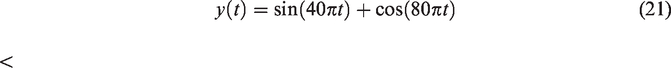
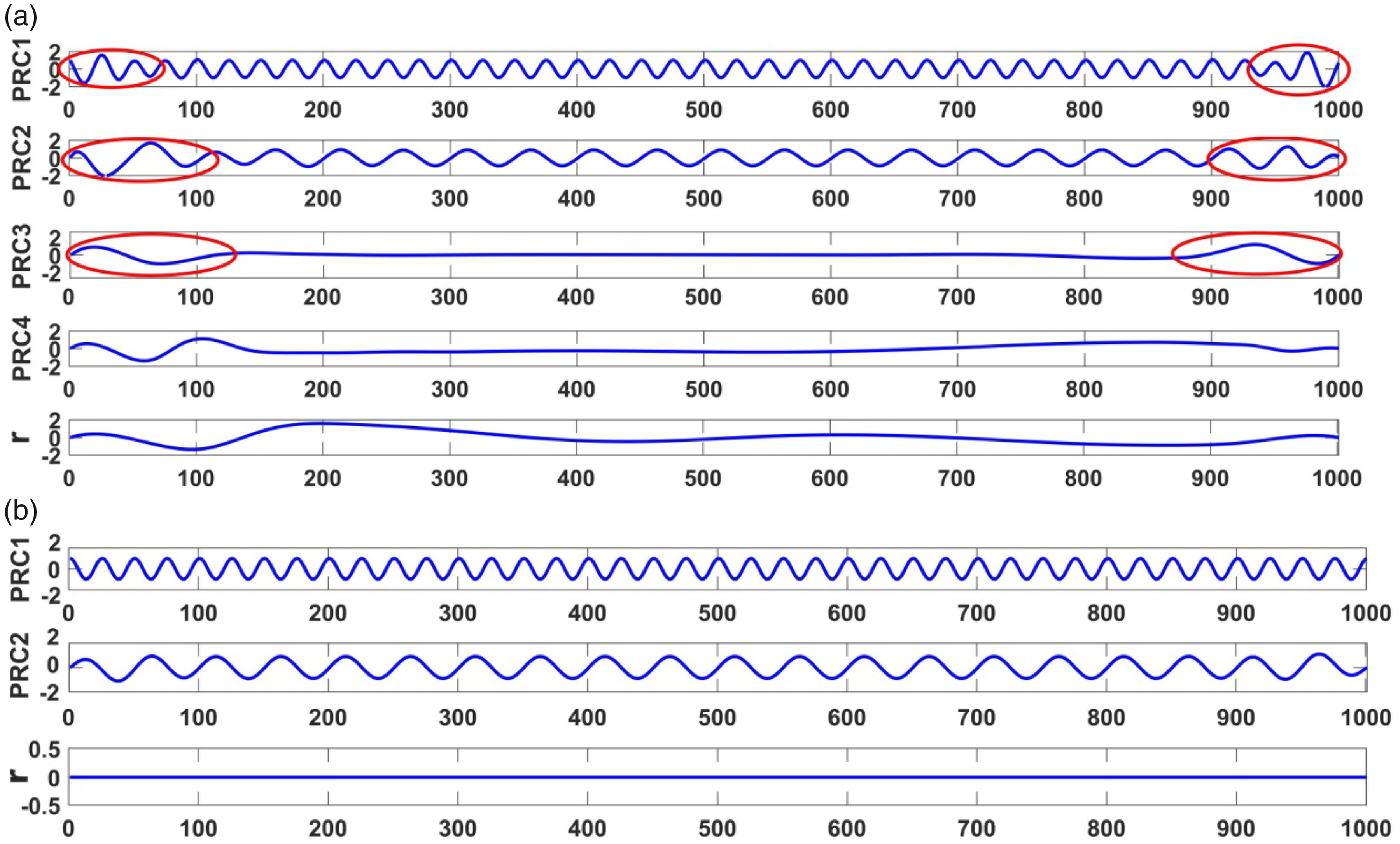
Gaussian noise information is added by simulation software. The two components with frequencies of 40 Hz and 20 Hz are defined as the first-order PRC and second-order PRC, respectively. When there is no noise, as shown in Figure 3, end effects occurred in Figure 3(a) by using the traditional ITD method. On the contrary, the wavelet-analysis-embedded ITD method could not only eliminate the end effects but also effectively reduce redundant PRCs (Figure 3(b)). As shown in Figures 4 and 5, a pure signal was obtained with the proposed method, and the proposed method has more advantages than the traditional ITD method in addressing the end effect problem. As illustrated in Figures 6 and 7, the enlargement of the (a) and (c) regions was shown in (b) and (d). Frequency–time representation is used to analyze the differences of PRC under the two methods. Figure 6 shows PRC1 and PRC2 with the corresponding error frequencies due to the end effect. The reason for this phenomenon is that the ITD method extracts the baseline signal based on the linear transformation, which may result in signal distortion, burr, and end effects. The comparative results in Figure 7 show that the wavelet-analysis-embedded ITD method was superior to the traditional ITD method in processing the distortion of signal and end effects effectively.
Signal decomposition. (a) Traditional ITD method. (b) WT combined with ITD method. PRC: proper rotation component.
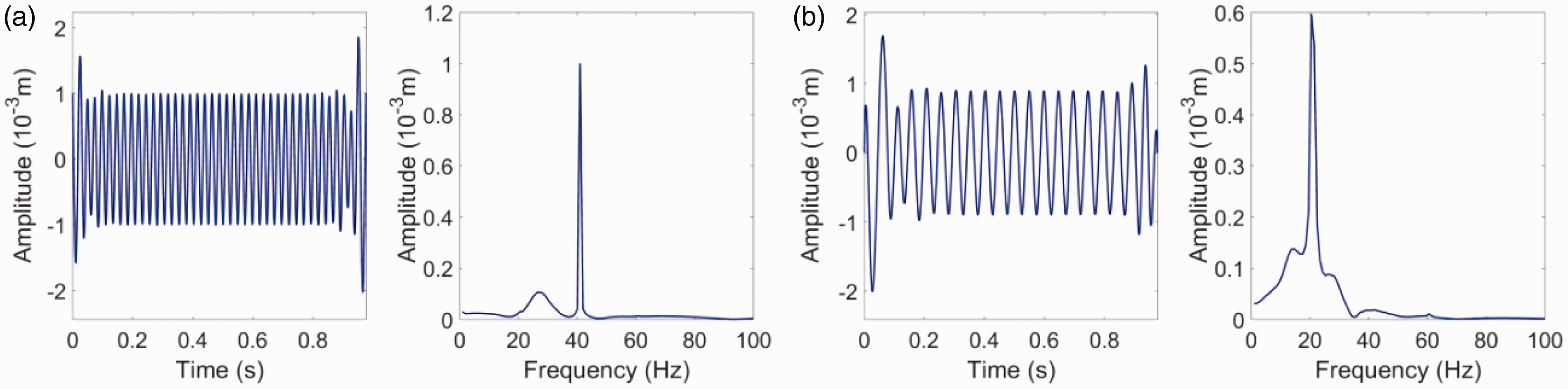
Time-domain and frequency-domain representation of PRC1 and PRC2, decomposed by the traditional ITD method. (a) PRC1. (b) PRC2. PRC: proper rotation component.
Time-domain and frequency-domain representation of PRC1 and PRC2, decomposed by proposed WT combined with the ITD method. (a) PRC1. (b) PRC2. PRC: proper rotation component.
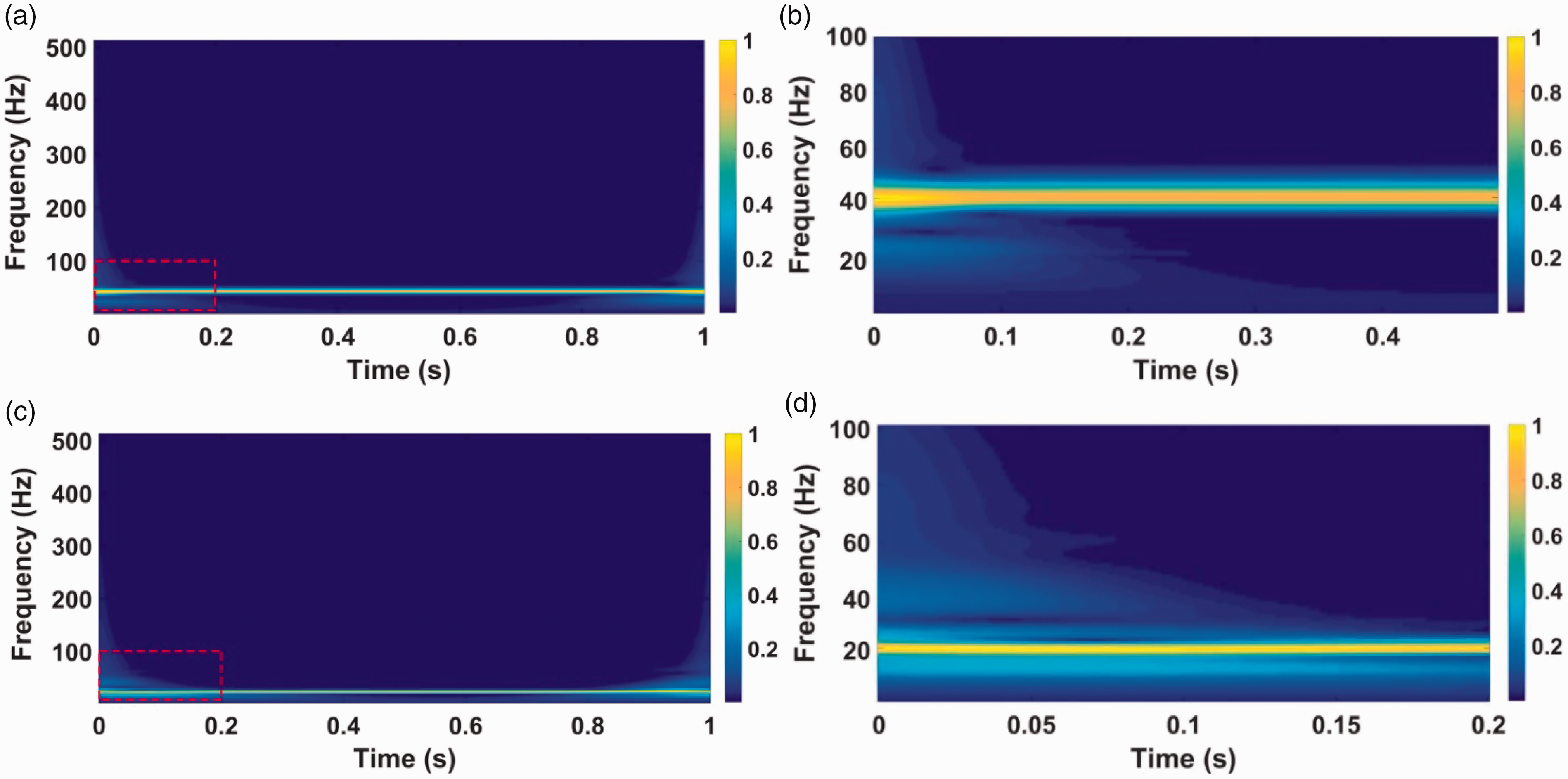
Frequency–time representation of PRC1 and PRC2 decomposed by the ITD method. (a) PRC1. (b) Red region of PRC1. (c) PRC2. (d) Red region of PRC2. PRC: proper rotation component.
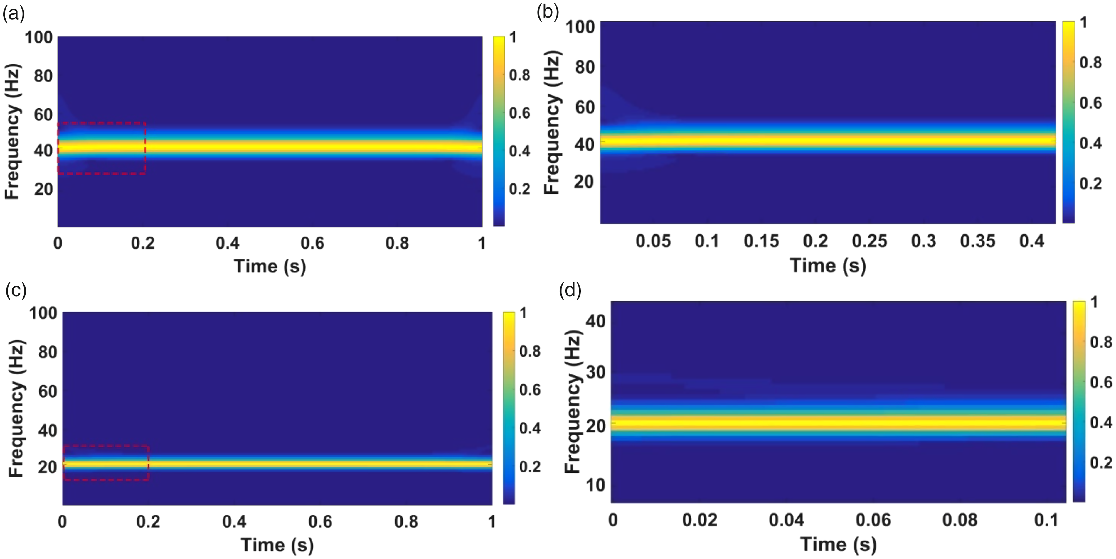
Frequency–time representation of PRC1 and PRC2, decomposed by the proposed WT combined with ITD method. (a) PRC1. (b) Red region of PRC1. (c) PRC2. (d) Red region of PRC2. PRC: proper rotation component.
After adding the noise, the traditional ITD method was applied to perform a comparison analysis with the SITD approach in terms of denoising and feature recognition, resulting in frequency aliasing in every PRC, as shown in Figure 8(a). Figure 8(b) is the representation after denoising with a hard threshold function, and the noise is basically filtered out, but over-smoothing leads to distortion in the signal details. Figure 8(c) shows the effect after denoising with a soft threshold function; the selected threshold value is half the threshold value used in Figure 8(b). The details of the signal are more evident than the result when using a hard threshold function for denoising; however, more noise is also retained. To preserve the signal details in the denoising procedure, it is necessary to design a new threshold function between the hard threshold function and the soft threshold function. The SITD algorithm filtered the background noise and extracted two weak PRCs from the investigated signal effectively (Figure 8(d)). The cross-correlation coefficients of the extracted PRCs and the real modes obtained by using the proposed method with different threshold function methods—soft threshold, 24 hard threshold, 25 and proposed adaptive threshold—are 0.7064, 0.7506, and 0.8654, respectively. The larger the coefficient value is, the better the extracted PRCs match the real signal mode.
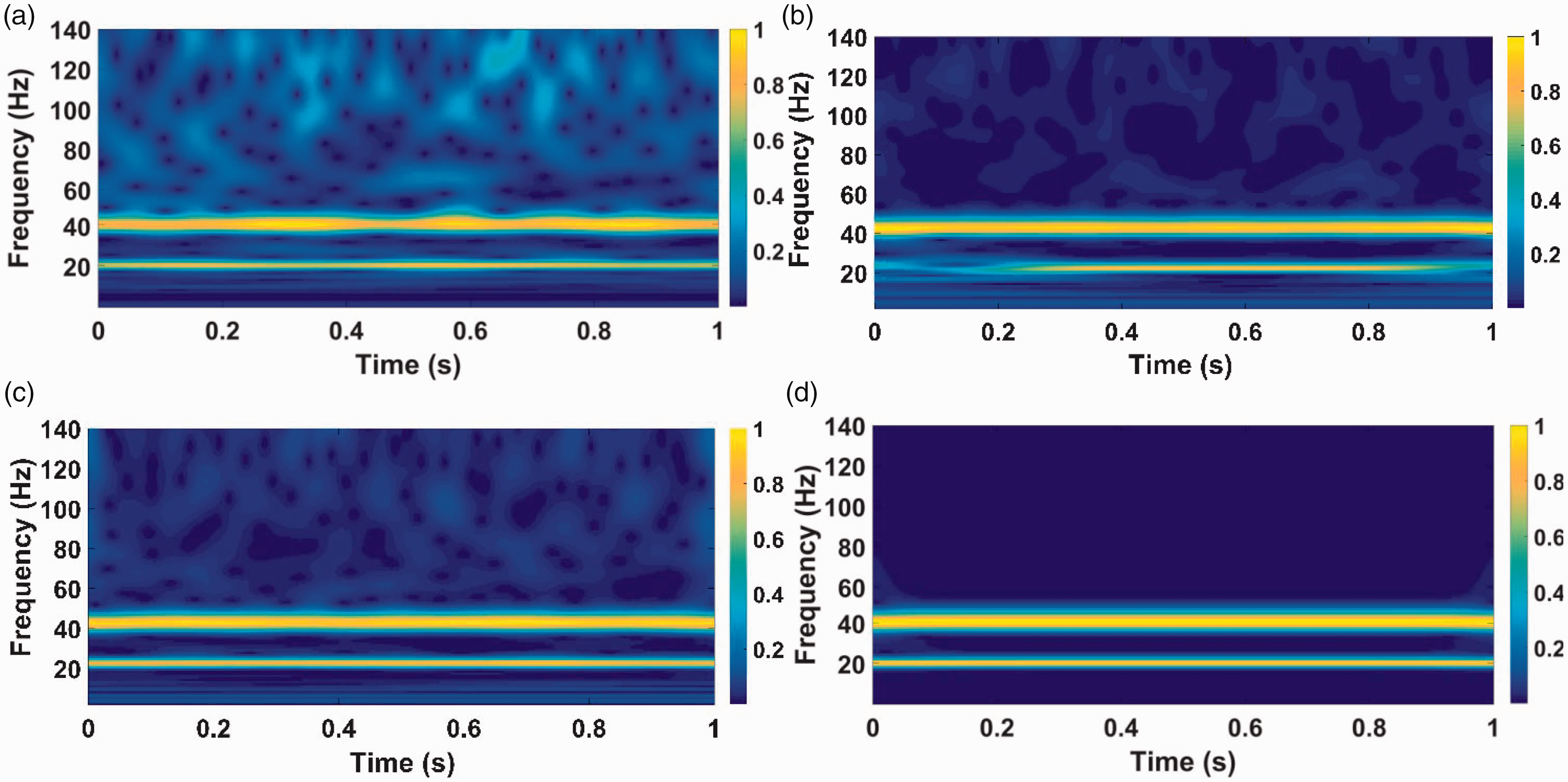
Frequency–time representation. (a) Decomposed by the traditional ITD method. (b) Decomposed by WT (hard threshold function) combined with the ITD method. (c) Decomposed by WT (soft threshold function) combined with the ITD method. (d) Decomposed by the proposed WT combined with the ITD method.
Experimental validation
The fault diagnosis approach for rolling bearings based on SITD and MF-DFA is presented in this part. The frame for fault identification is shown in Figure 9. Firstly, the original signal was decomposed into several PRCs by applying SITD method. Secondly, the instantaneous amplitude in each PRC was analyzed by MF-DFA, and the multi-fractal features were represented by the generalized Hurst exponents. The generalized Hurst index of different q was obtained. Thirdly, LLTSA was used to decrease the value of dimension. The feature vector was formed by applying the major influencing components got from LLTSA. Fault diagnosis of rolling bearing was realized by verifying the extracted fault feature vectors.
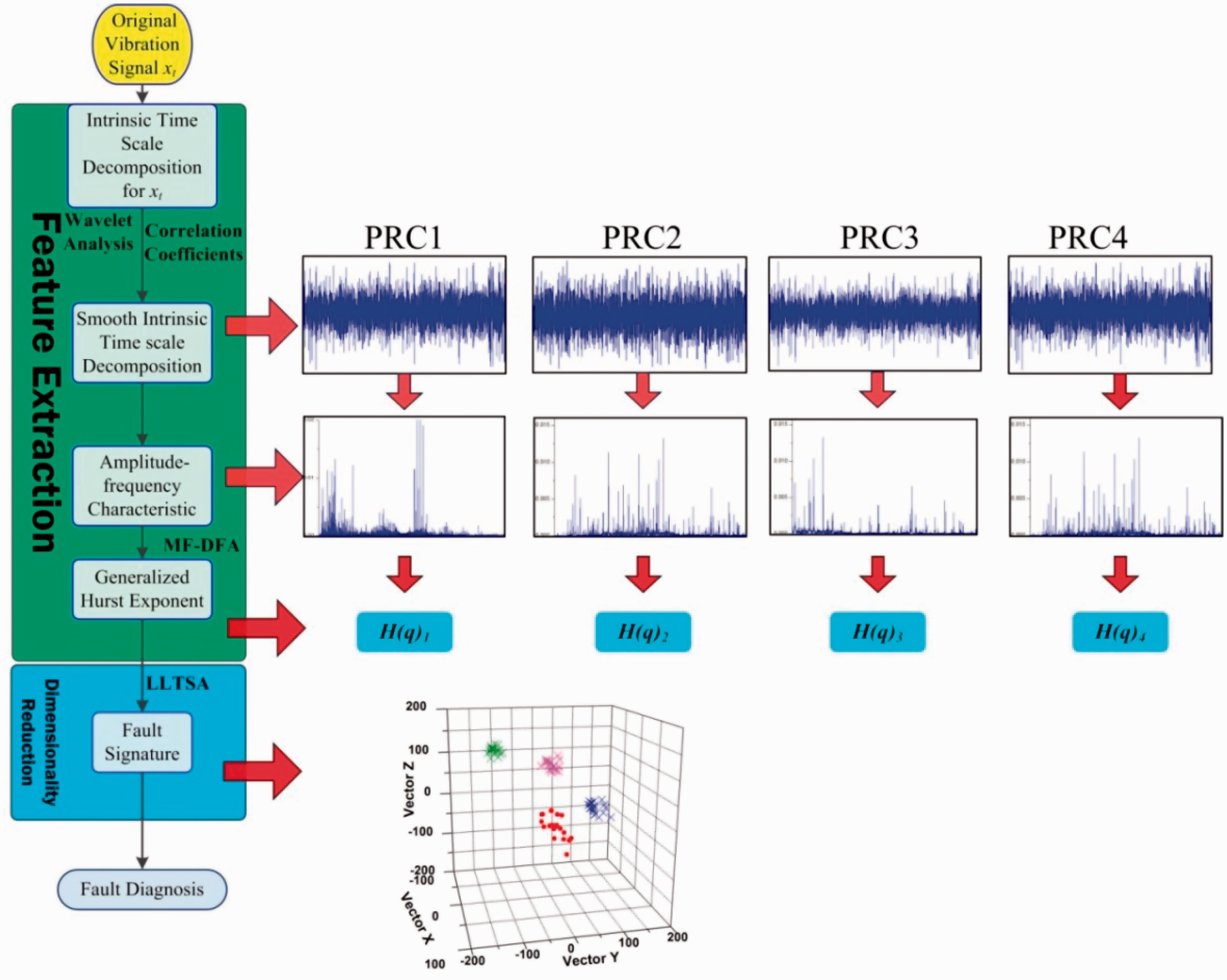
The scheme for fault identification. PRC: proper rotation component; LLTSA: linear local tangent space alignment; MF-DFA: multi-fractal detrended fluctuation analysis.
Feature extraction by applying SITD and MF-DFA
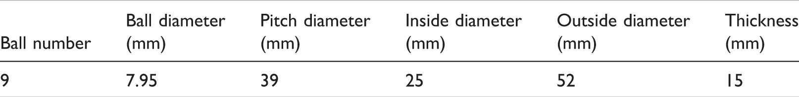
The proposed SITD method was used to extract the fault characteristics of the vibration signal from Case Western Reserve University. The experiment platform is shown in Figure 10(a) 2 hp Reliance Electric motor, torque encoder, and dynamometer), and the bearing information is listed in Table 1. The motor drives input and output shaft drive loads of 1, 2, 3, and 4 hp. EDM (electrical discharge machining) technology is used to produce single-point faults on the test bearings with different fault diameters (0.1778, 0.3556, and 0.5334 mm). The sampling frequency is 12 kHz.
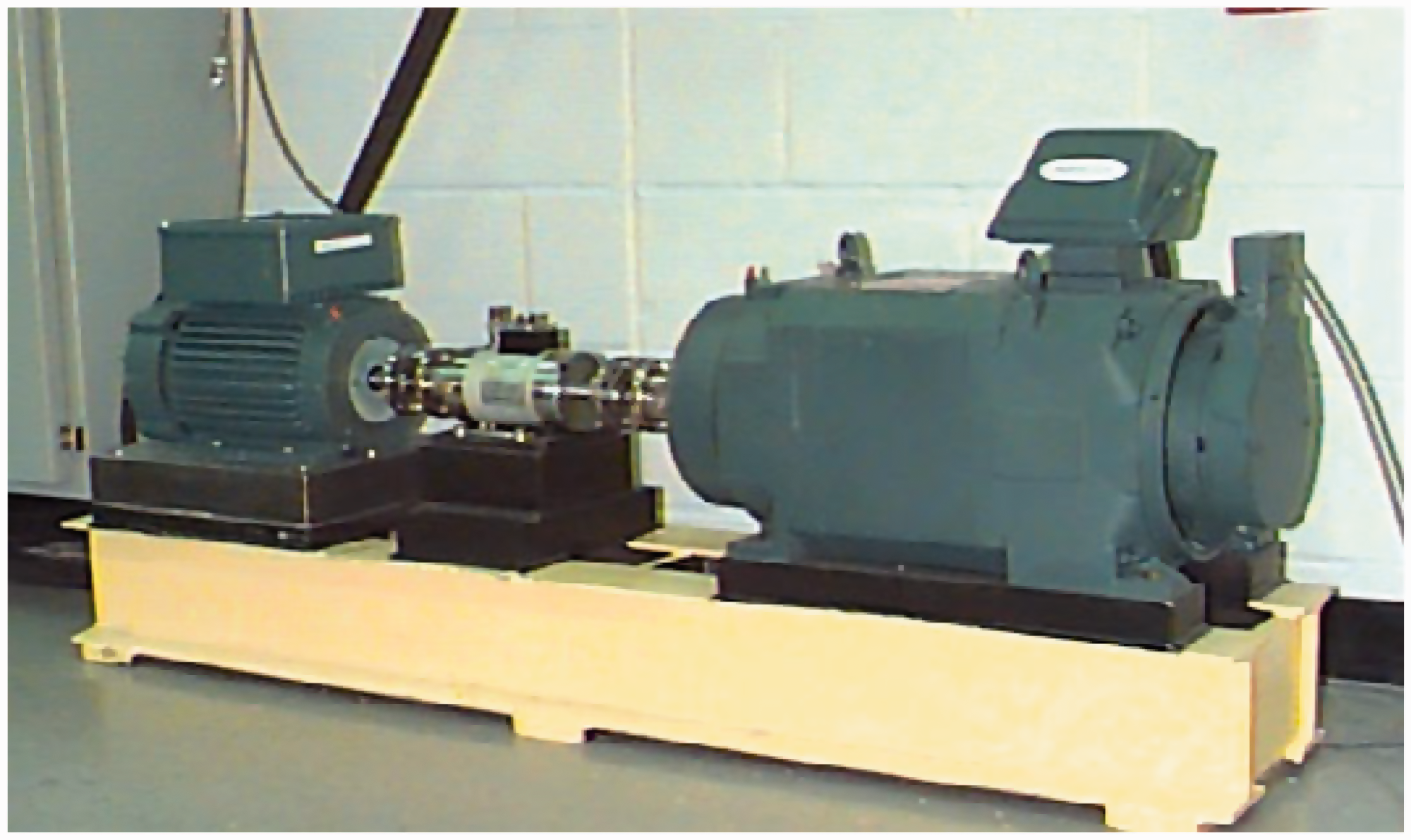
Test platform of rolling bearings.
Test rolling information.
The original signal was decomposed into multiple PRC signals by applying SITD. According to SITD decomposition, the first few PRCs exhibit the largest energy and frequency. In other words, the first few PRCs contain most of the effective signal information. With regard to this point, only the first four PRCs were preserved in this study.
To verify the applicability of the proposed method of the actual working situation, Gaussian white noise was added. Figure 11 depicts the time-domain representation of the inner-race fault signal and contaminated signal, which is composed of an inner-race fault signal and Gaussian white noise. The multi-fractal characteristics of each instantaneous amplitude matrix were analyzed by using MF-DFA. The scale index q of MF-DFA used in this study is −2, −1, 0, 1, and 2.
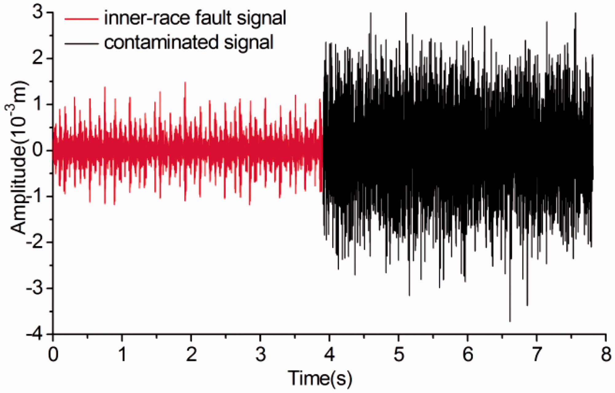
Time-domain diagram.
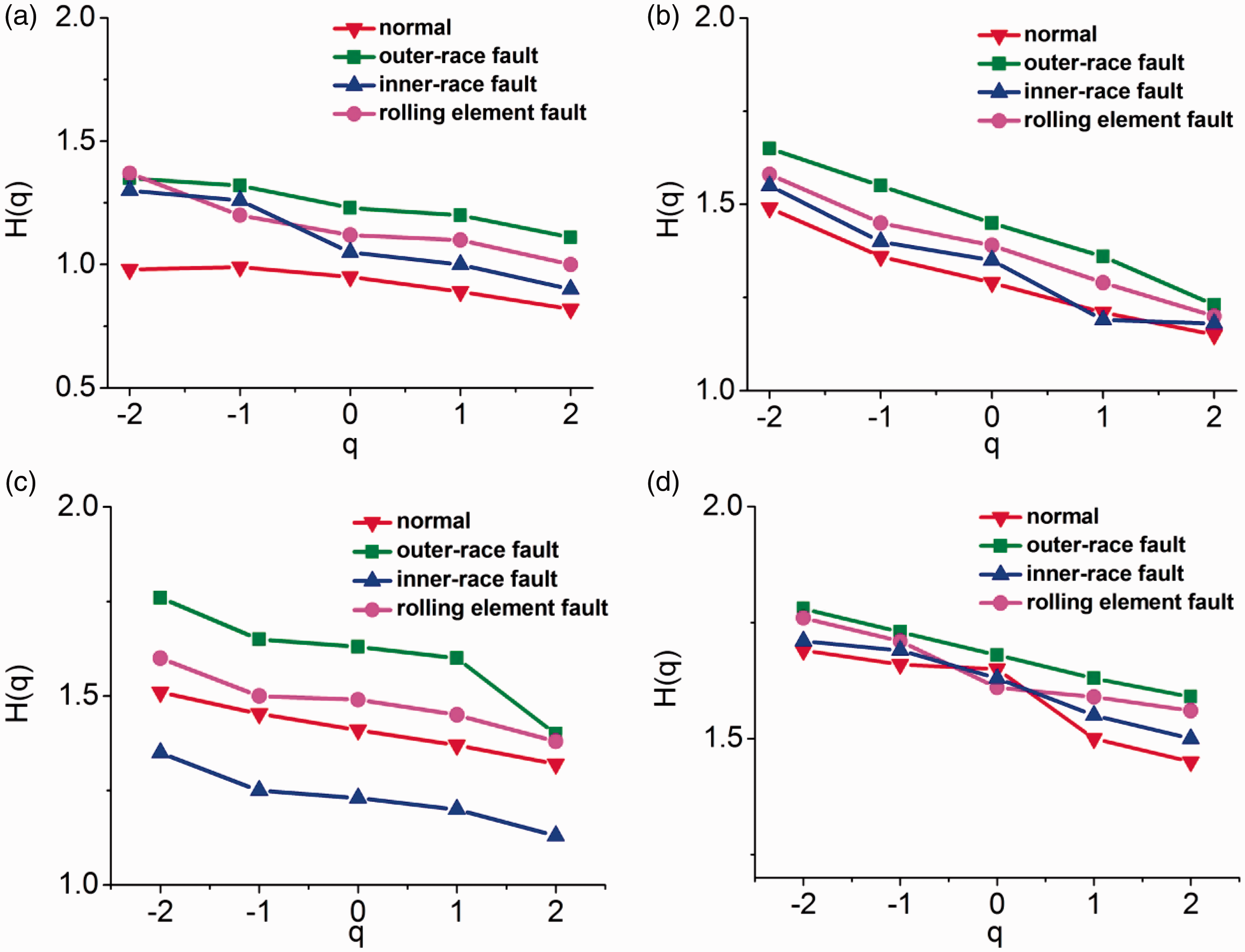
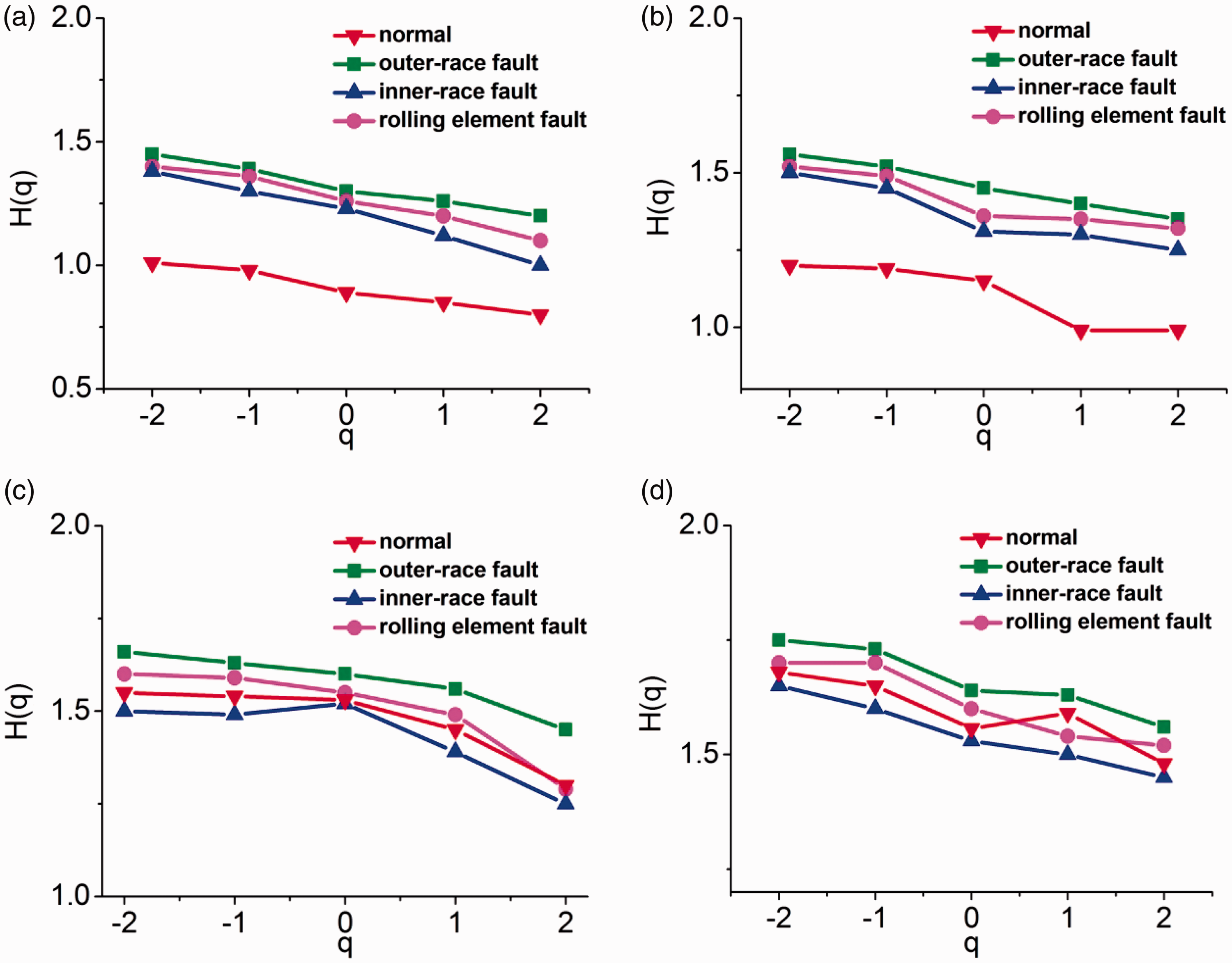
Figures 12 to 14 describe the generalized Hurst exponents for PRC1, PRC2, PRC3, and PRC4 in four different states (normal, outer-race fault, inner-race fault, rolling-element fault) with three different failure diameters (0.1778, 0.3556, and 0.5334 mm, respectively).
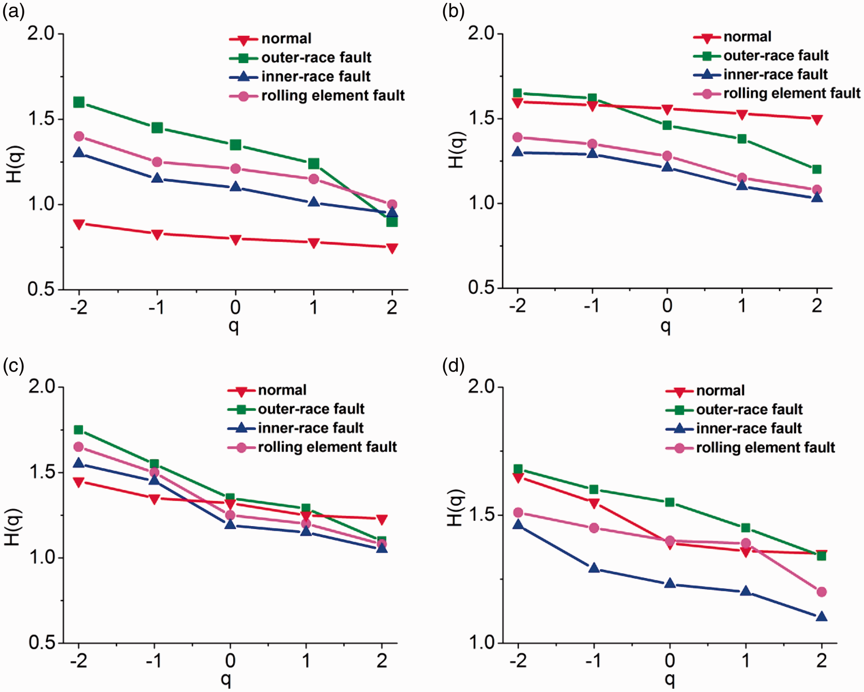
Generalized Hurst exponent of first four PRCs with a fault diameter of 0.1778 mm. (a) PRC1. (b) PRC2. (c) PRC3. (d) PRC4. PRC: proper rotation component.
Generalized Hurst exponent of first four PRCs with a fault diameter of 0.3556 mm. (a) PRC1. (b) PRC2. (c) PRC3. (d) PRC4. PRC: proper rotation component.
Generalized Hurst exponent of first four PRCs with a fault diameter of 0.5334 mm. (a) PRC1. (b) PRC2. (c) PRC3. (d) PRC4. PRC: proper rotation component.
As can be seen from the figures, the generalized Hurst components of various states were distinguished. In summary, the various rolling bearing states have different multi-fractal features.
Application of LLTSA to rolling bearing dimension reduction
In this study, the first four PRCs presented in the previous section were chosen and analyzed by the MF-DFA method. The number of multi-fractal features H(q) is 5 for the instantaneous amplitude corresponding to each PRC (q = [−2, −1, 0, 1, 2]). Its total number is 20 for each set of data.
For rolling bearing diagnostic systems, the large number of features may decrease their robustness and may even result in a decrease in diagnostic accuracy. LLTSA is a type of algorithm used for dimensionality reduction.26–29 Its purpose is to extract the major influencing factors. In this study, LLTSA projected the multi-fractal features into a three-dimensional space.
Diagnostic performance under different operating conditions
A change in velocity will affect the fault characteristic frequency. The characteristics extracted by the traditional method fluctuate greatly under variable working conditions, which may lead to the mixing of feature vectors of different fault states and reduce the diagnostic accuracy. Considering these statements, it is indispensable to study the diagnostic characterization of the method under different circumstances (motor speeds of 1797, 1772, 1750, and 1720 r/min, respectively).
The normal state data set contains 80 groups. Every single fault data set is separated into 12 subsets under four different working conditions (load of output shaft drive is 1, 2, 3, and 4 horsepower) and three different faults diameters (0.1778, 0.3556, and 0.5334 mm); each subset contains 20 groups, and each group contains 4096 points. The data set information is shown in Table 2. Figures 15 to 17 exhibit the scatter plots of the three vectors.
Information of the data set.
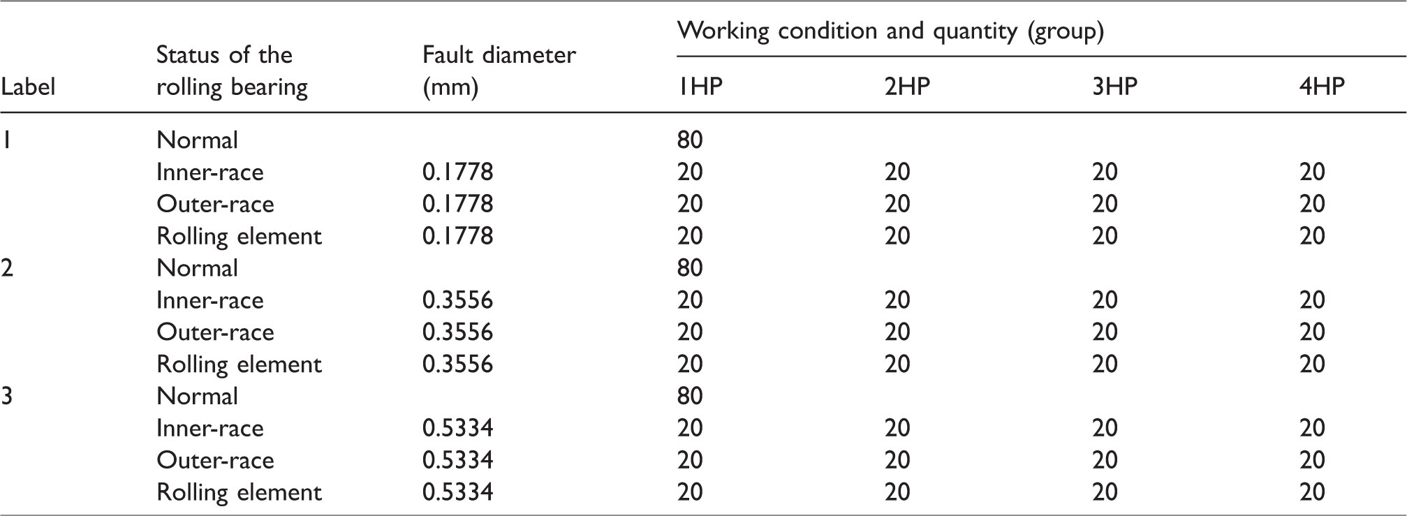
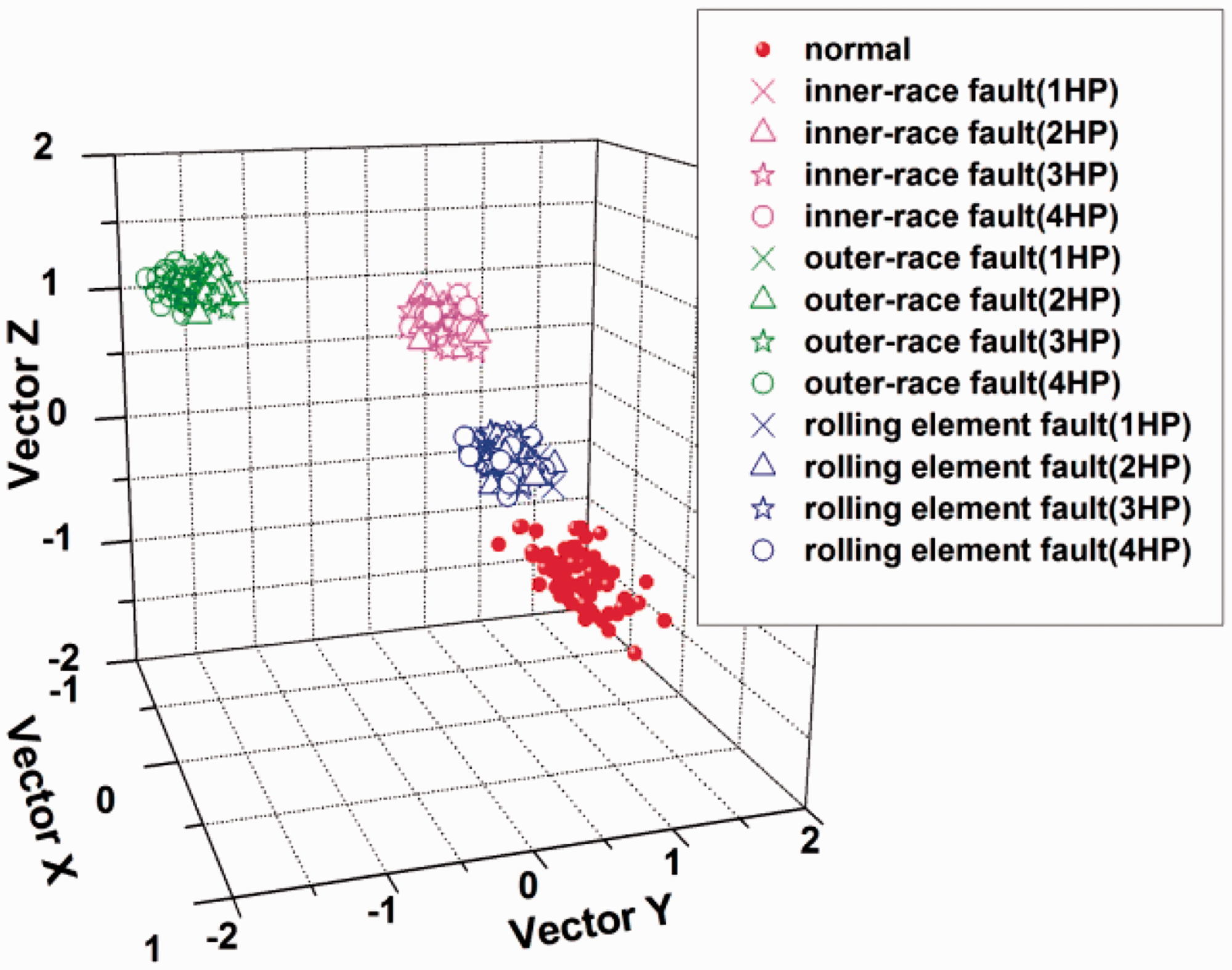
Diagram of the clustering result of Data set 1 (SITD + MF-DFA).
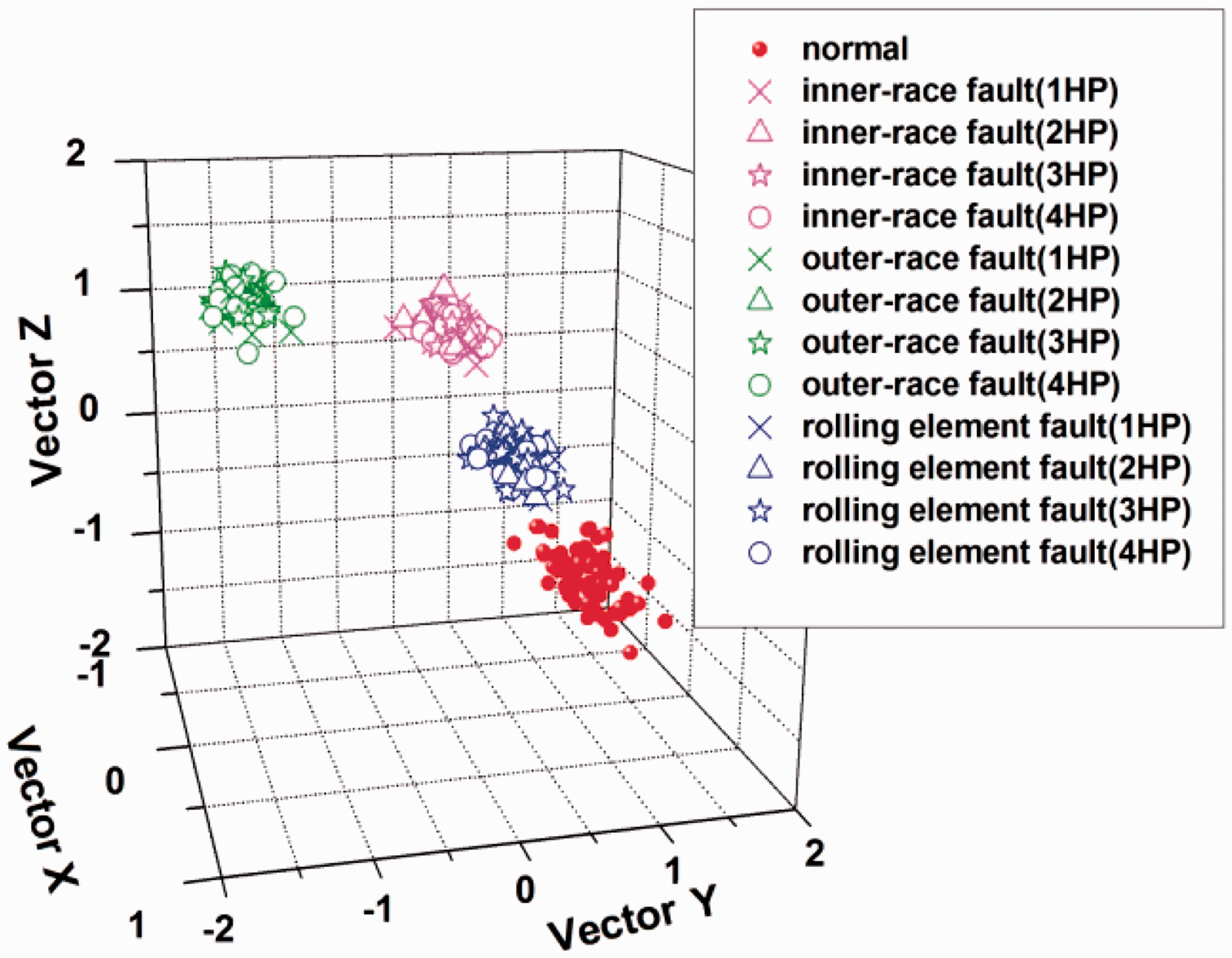
Diagram of the clustering result of Data set 2 (SITD + MF-DFA).
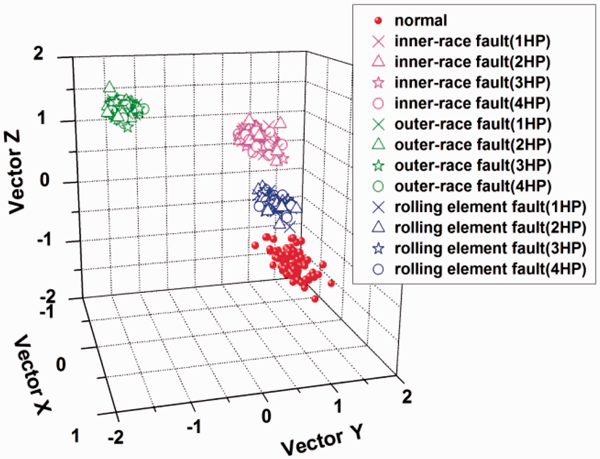
Diagram of the clustering result of Data set 3 (SITD + MF-DFA).
As can be seen from the figures, there is no mixing of feature vectors of different fault states (normal, inner-race fault, outer-race fault, rolling element fault). In other words, a fluctuation in working conditions has no effect on the extracted feature vectors that were verified in the situations of different fault diameters. The signals processed by the ITD-MF-DFA method are shown in Figures 18 to 20, in which the extracted feature vectors in different fault states are combined with each other.
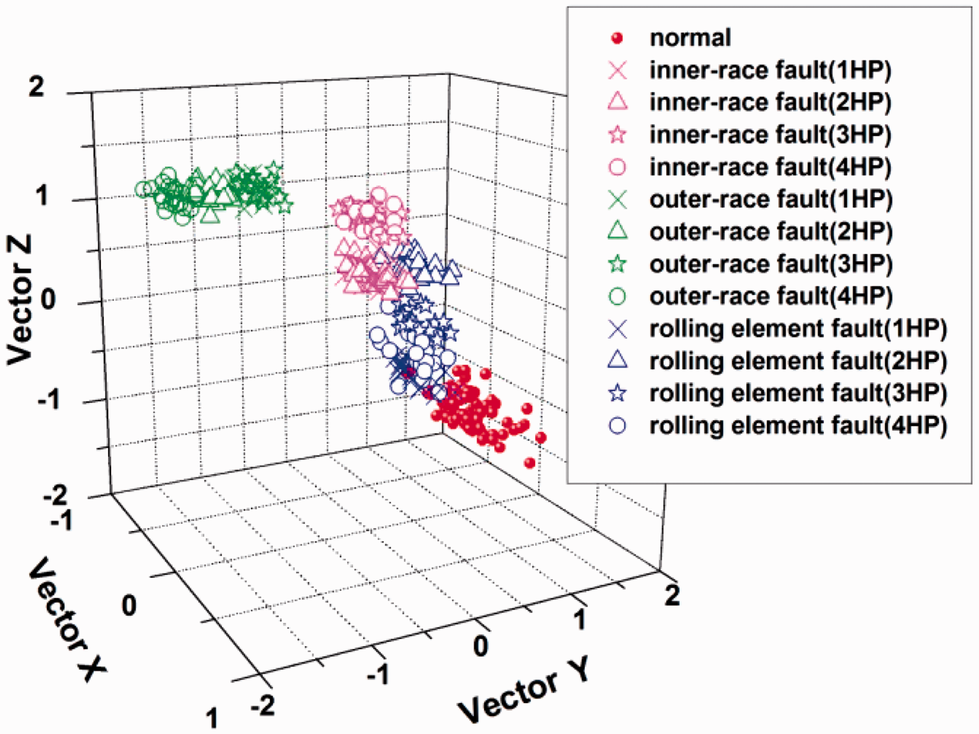
Diagram of the clustering result of Data set 1 (ITD + MF-DFA).
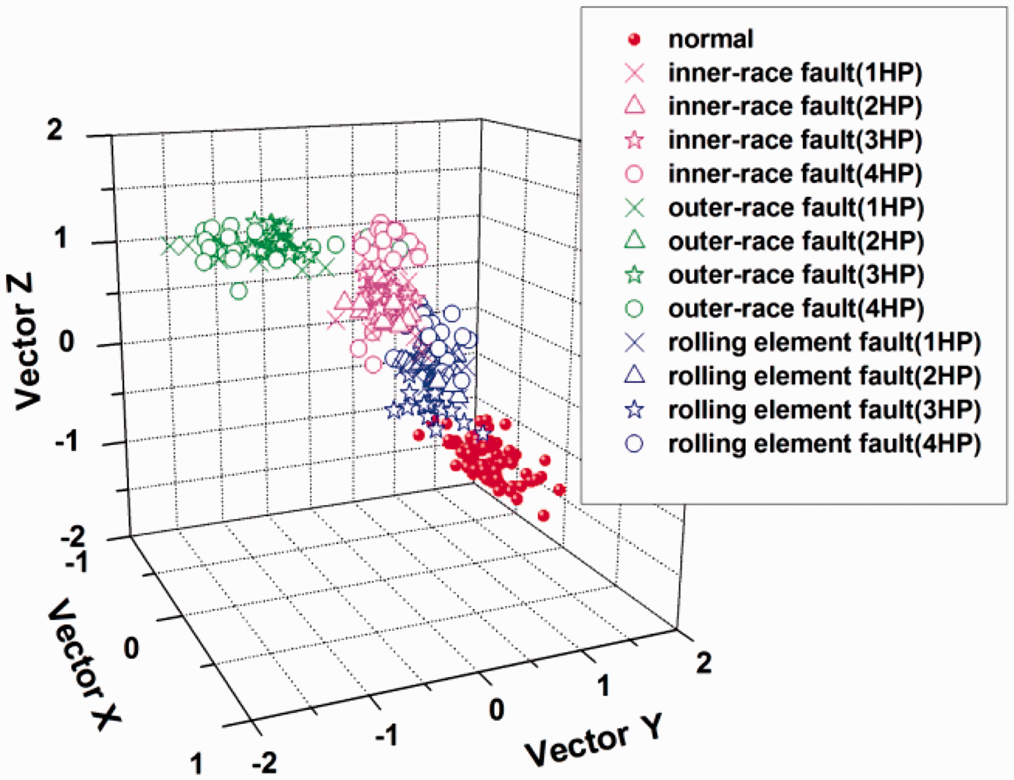
Diagram of the clustering result of Data set 2 (ITD + MF-DFA).
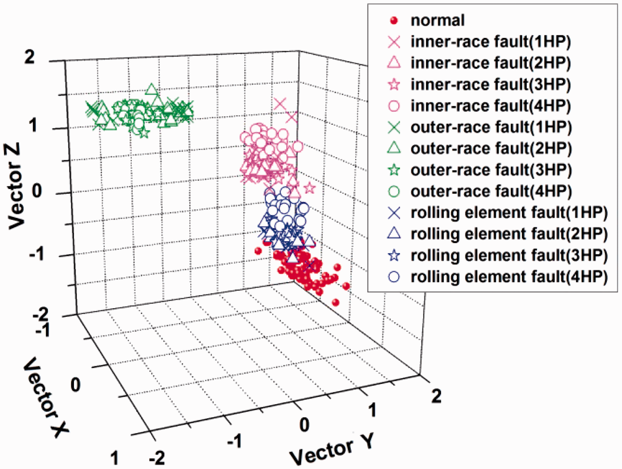
Diagram of the clustering result of Data set 3 (ITD + MF-DFA).
Conclusions
To improve the accuracy of feature extraction in fault diagnosis, a new fault diagnosis approach involving rolling bearing decomposition based on SITD and MF-DFA was proposed. Comparative studies indicate that the SITD approach is superior to traditional ITD methods in treating the noise interference problem. After signal processing by SITD, the first four PRCs were selected to implement MF-DFA to exhibit the intrinsic multi-fractality in the instantaneous amplitude of the extracted PRCs. The multi-fractal features were represented by the generalized Hurst exponents. Finally, LLTSA was used to decrease the value of the dimensions, and the main multi-components are screened to construct feature vectors. The diagnostic performance under different operating conditions is studied. Experimental results show that the proposed approach is feasible for recognizing the rolling bearing fault types.
This method has the following characteristics: (1) the proposed method effectively eliminates noise interference and inhibits end effects; (2) the algorithm increases the SNR, improving the accuracy of feature extraction when the MF-DFA method is used in fault diagnosis; and (3) the method can be applied to the fault diagnosis of rolling bearings and the accurate identification of the fault types effectively.
Footnotes
Acknowledgements
The authors greatly appreciate the constructive comments provided by the anonymous reviewers and the editors.
Declaration of conflicting interests
The author(s) declared no potential conflicts of interest with respect to the research, authorship, and/or publication of this article.
Funding
The author(s) disclosed receipt of the following financial support for the research, authorship, and/or publication of this article: This research is sponsored by Natural Science Foundation of Liaoning Province, China (Grant Nos. 20180550927 and 20180550002); National Natural Science Foundation of China (Grant No. 51705342); and National Key Research and Development Program of China (2017YFC0703903).