Vibro-acoustic coupling characteristics of orthotropic L-shaped plate–cavity coupling system

Abstract

The research object of this paper is the L-shaped plate–cavity coupling system established by a cuboid acoustic cavity with rigid-wall or impedance-wall and L-shaped plate with numerous elastic boundary conditions in view of the Fourier series method. The main research content of this paper is the vibro-acoustic coupling characteristics. In this paper, the displacements admissible functions of the L-shaped plate are generally set as the sum of two cosines’ product and two polynomials. Sound pressure admissible functions of the cuboid acoustic cavity can be considered as the sum of three cosines’ product and six polynomials. The discontinuity of coupling system at all boundaries in the overall solution domain is overcome in this way. Through the energy principle and the Rayleigh-Ritz technology, it can be got that the solving matrix equation of the L-shaped plate-cavity coupling system. Based on verifying the great numerical characteristics of the L-shaped plate–cavity coupling model, they obtained both the frequency analysis and the displacement or sound pressure response analysis under the excitation, including a unit simple harmonic force or a unit monopole source. The advantages of this method are parameterization and versatility. In addition, some new achievements have been shown, based on various materials, boundary conditions, thicknesses, and orthotropic degrees, which may become the foundation for the future research.

Introduction

In recent years, the plate–cavity coupling structures have been widely applied in transportation vehicles such as airplanes, ships, and automobiles. The study of the plate–cavity coupling mechanism is very important. The research status of the coupled plate and the coupled plate–cavity system is mainly introduced in this section.

Some literatures about the L-shaped coupled plate structures are listed here. Boisson et al. ¹ discussed the relationship between factors such as thickness, damping, area and excitation type, and the vibration energy transmission characteristics. Kim et al. ² used a modal analysis way to study the energy situation in coupling rectangular plates in middle or high frequency ranges. Shen and Gibbs ³ expressed the vibration displacement function and obtained the displacement value of the coupling plate. All factors, including the excitation force position, excitation frequencies, boundary conditions (BC), and material parameters, were studied taking into consideration the response of the coupling plate. Chen and Sheng ⁴ applied a mobility power flow method and determined natural frequency of the L-shaped coupled plate. The above articles investigate different tools to consider the vibration characteristics of the coupling plate. But the existing theoretical analysis of the L-shaped coupled plate considers the bending moment between the elastic plates, while ignoring the lateral shear, longitudinal, and in-plane shearing effects in the plate. Studies have shown that large deviations occur in the displacement response of the coupled plate structure using the modeling technique that does not include the in-plane vibration component. Therefore, it is very important to establish a more general vibration model.

The L-shaped plate and cuboid cavity coupling system is the emphasis of this paper. Most of the current research is focused on the single-plate coupled with cuboid acoustic cavity. Pirnat et al. ⁵ proposed a rectangular single plate–cavity model with point sound source. Chen et al. ⁶ presented a general plate–cavity coupling modeling method to analyze the vibro-acoustic characteristics. Koshigoe et al. ⁷ applied a plate–cavity coupling model to study active control of sound transmission. Sadri and Younesian ⁸ studied harmonic response about the plate–cavity system. Hamdi et al. ⁹ studied the vibration of the plate–cavity model by using a displacement method. Sum and Pan ¹⁰ proposed a mathematical description which allowed the acoustic modal cross-coupling and structural modal cross-coupling to be studied independently. David and Menelle ¹¹ expressed a numerical method to verify the natural features of the coupling system. Nefske et al. ¹² summarized the finite element method (FEM) for plate–cavity coupling structures and investigated the acoustic properties of vehicles with closed structures. Du et al. ¹³ analyzed a plate–cavity system composing of the cuboid cavity with rigid wall and the plate with elastic BC. Li and Cheng ¹⁴ introduced characteristics of plate–cavity coupling system by utilizing fully coupled vibro-acoustic model. Guy ¹⁵ employed the multimodal analysis method to point out the response about the plate–cavity coupling system under point sound source. Pan and Bies ¹⁶ considered the effects of fluid–structural coupling when analyzing the sound pressure. Ang et al. ¹⁷ discussed the effects of material kinds and geometric sizes on the vibro-acoustic characteristics. Frendi et al. ¹⁸ described the numerical calculation of plate–cavity coupling system. Pretlove ¹⁹ dealt with forced vibrations of plate–cavity coupling system by using theory for free vibration. Suzuki et al. ²⁰ examined boundary vibration velocities by calculating with the structural–acoustic coupling effect. Pates et al. ²¹ harnessed the method that combined boundary element with the FEM to accurately model plate–cavity interaction of a composite plate resting on an acoustic cavity. Maxit ²² used a dual modal formulation to analyze the response of plate–cavity coupling system. Wang ²³ introduced a power flow analysis of finite coupled plate using the method of reverberation-ray matrix. Jain and Sonti ²⁴ proposed a matrix analytical solution to obtain the coupled resonances of plate–cavity coupling system. Cui et al. ²⁵ analyzed the coupled sound field problem by the modal analysis method. Dozio and Alimonti ²⁶ proposed a variable structure finite element analysis model to study the acoustic vibration characteristics of plate–cavity coupling system. Sarıgül and Karagözlü ²⁷ studied the structural–acoustic system of a rectangular plate structure coupled with a rigid wall acoustic cavity. The above papers give several modeling methods and related numerical algorithms and analyze the forced responses. As can be seen from the above research literature, there are some defects in the existing research. The factors considered in the modeling process of the plate–cavity system are not complete. The lateral shear, longitudinal, and in-plane shear effects in the plate are not ignored during the modeling of this paper. In order to better comprehend this more complex coupling phenomenon, a more comprehensive forecasting model needs to be established.

The vibro-acoustic characteristics of the multi-layer plate-cavity coupling system have also attracted researchers' attention. Xin et al. ²⁸ harnessed the vibro-acoustic properties of a square double-plate with the clamped BC in an infinite acoustic rigid wall by adopting a double Fourier series method. Lee ²⁹ obtained the natural frequencies of the cuboid cavity. Li and Chen ³⁰ proposed a study on the plate–cavity–plate characteristics by using modal superposition method. Carneal and Fuller ³¹ and Chazot and Guyader ³² conducted theoretical and experimental studies on the acoustic energy transfer of double-layer plates on simply supported boundaries. Tanaka et al. ³³ solved the eigenvalue problem of the coupling system with various coupling conditions. Cheng and Ji ³⁴ proposed a Chebyshev–Ritz based analytical model to study plate–cavity system. The multi plate–cavity coupling system is mainly considered at this stage. They are less than the researches about the L-shaped plate–cavity coupling system. Therefore, the studies about the line coupling and the surface coupling are rare.

It can be seen from the above research literature that they mainly study the coupling structures based on classical BC and isotropic materials. But there are some defects in the existing research. Specially, the factors of the coupling relationship are incomplete during the modeling of the L-shaped plate-cavity system. Many articles do not consider the phenomenon of large deviation in the displacement response of the coupling plate structure caused by ignoring transverse shear, longitudinal, and in-plane shear effects in the plate. In order to better study this more complex structure–acoustic coupling phenomenon, more comprehensive forecasting model needs to be established. The Fourier series method ³⁵ has good properties such as convergence and orthogonality. The Rayleigh–Ritz technology ³⁶ is a method of solving the unknown function by the stationary condition of energy functional. Therefore, it is established that a vibro-acoustic examine model of the L-shaped plate and the cuboid cavity coupling system is based on the improved Fourier series method and Rayleigh energy technology.^37–39 This method overcomes the discontinuity of the L-shaped plate–cavity coupling system at many boundaries in an entire solution domain. The significance of this method is to facilitate parameterization research and commonality. Furthermore, some results are attained through examining the influence of factors including various materials including isotropic and orthotropic, plate thicknesses, and orthotropic degrees. This model has obvious advantages in dealing with displacement and sound pressure response.

Theoretical knowledge

Description of the L-shaped plate–cavity coupling system

The model composes of the L-shaped plate that has any BC and a cuboid acoustic cavity which has various impedance walls (Figure 1). And this makes it easy to develop the vibro-acoustic coupled characteristics. From Figure 1, the x, y, and z in the coordinate system, respectively, represent length, width, and height directions of the L-shaped plate and the cuboid cavity coupling system. The geometric sizes of the coupling system are a₁, b, and a₂. The length, width, and thickness of plate 1 and plate 2 can be, respectively, noted as a₁, b, and h₁ and a₂, b, and h₂. The L-shaped coupled plate structure is formed by connecting a common boundary of the plate 1 and the plate 2 (x₁=0 or x₂=a₂). Among them, the plate 1 is located in the plane of x₁–y₁. The BC of the bending vibration can be imitated by the linear and the rotational springs that are uniformly distributed along the boundary. Analogously, the BC of the in-plane vibration are imitated by the linear springs that are uniformly distributed along the boundary in the plane of x₁–y₁. For example, for the boundary at x₁=a₁, the symbols k_bx11 and K_bx11 represent the stiffness coefficient of the linear and the rotational springs, which are used to simulate bending vibration. The symbols k_nx11 and k_px11 represent the stiffness coefficient of the linear springs, which are used to simulate in-plane vibration. The x₁–y₁–z₁ is selected as the primary coordinate. And the relative position between the plates 1 and 2 can be described by defining the coupling angle $\theta$ . When the coupling angle is 90 degrees, the two plates at this time form the L-shaped plate. The coupling BC can be set by using four types of coupling springs (represented by K_c, k_c1, k_c2, and k_c3) that are uniformly distributed along the coupling boundary. The four types of coupling springs consider four coupling behaviors of transverse bending moment, outer-plane shearing, and inner-plate shearing of x and y directions. The BC are set by eight types of springs, which are linear springs (k_bxij, k_pxij, k_nxij, k_c1, k_c2, and k_c3) and rotational springs (K_bxij and K_c), respectively. By introducing inconsistent stiffness values of the eight different springs, the any BC can be achieved. The point sound source Q and the point force F can be used for research of the sound pressure and displacement response.

Figure 1.

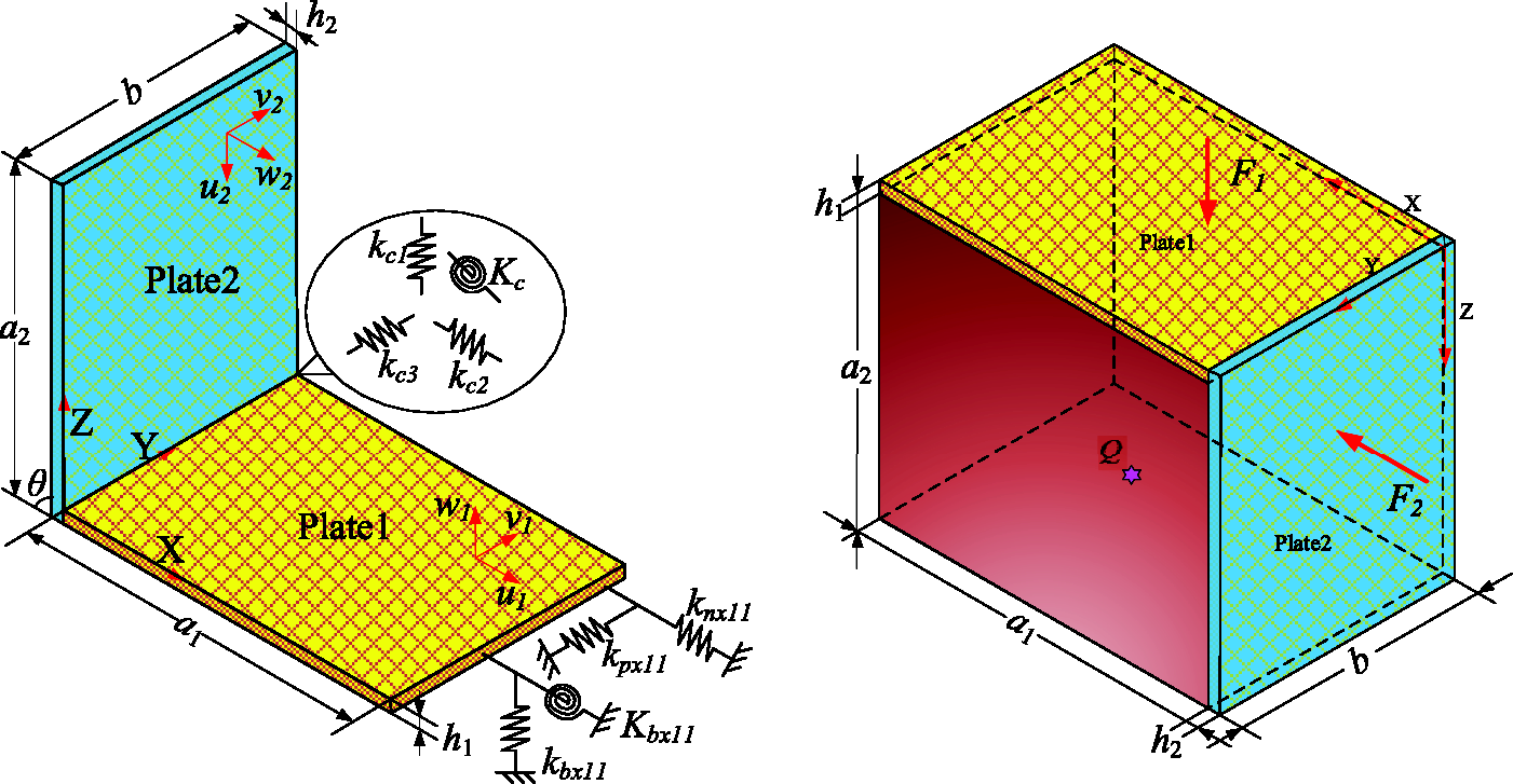
Coordinate system and geometry model of the L-shaped rectangular plate–cavity coupling system.

Admissible displacement and sound pressure functions

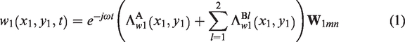
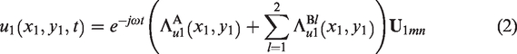
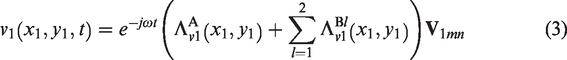
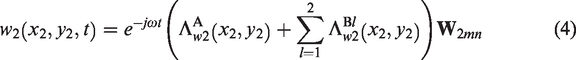
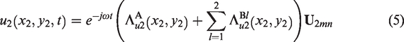
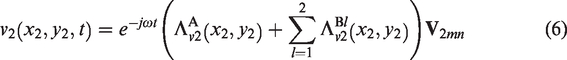
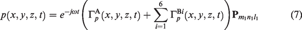
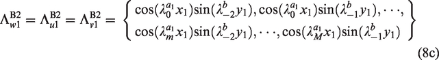
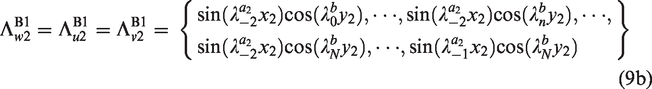
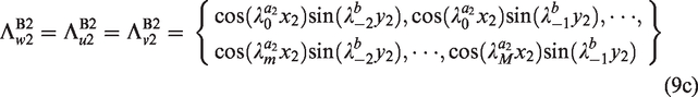
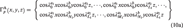
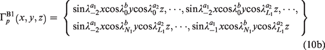
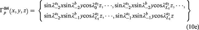
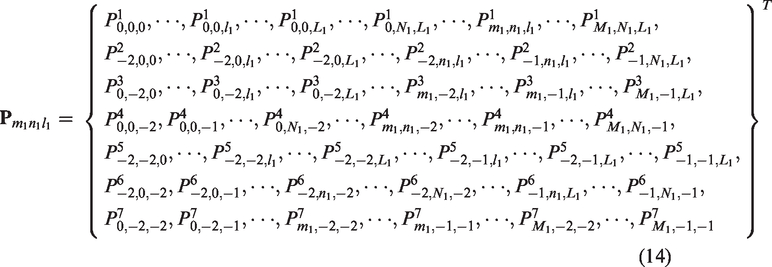
By introducing the Fourier series method, the displacements admissible functions of the L-shaped plate are generally set as the sum of two cosines’ product and two polynomials. The sound pressure admissible functions can be written as the sum of three cosines’ product and six polynomials.^40–42 The advantage of this method is that it helps to clear up the phenomenon of the boundary discontinuities. The displacements functions of the L-shaped coupled plate and the sound pressure functions of cuboid cavity can be written as follows

$$w_1\left(x_1,y_1,t\right)=e^{-j\omega t}\left({\mathbf{\Lambda }}_{w1}^{\text{A}}\left(x_1,y_1\right)+{\displaystyle \sum _{l=1}^2{\mathbf{\Lambda }}_{w1}^{\text{B}l}\left(x_1,y_1\right)}\right){\mathbf{W}}_{1mn}$$

(1)

$$u_1\left(x_1,y_1,t\right)=e^{-j\omega t}\left({\mathbf{\Lambda }}_{u1}^{\text{A}}\left(x_1,y_1\right)+{\displaystyle \sum _{l=1}^2{\mathbf{\Lambda }}_{u1}^{\text{B}l}\left(x_1,y_1\right)}\right){\mathbf{U}}_{1mn}$$

(2)

$$v_1\left(x_1,y_1,t\right)=e^{-j\omega t}\left({\mathbf{\Lambda }}_{v1}^{\text{A}}\left(x_1,y_1\right)+{\displaystyle \sum _{l=1}^2{\mathbf{\Lambda }}_{v1}^{\text{B}l}\left(x_1,y_1\right)}\right){\mathbf{V}}_{1mn}$$

(3)

$$w_2\left(x_2,y_2,t\right)=e^{-j\omega t}\left({\mathbf{\Lambda }}_{w2}^{\text{A}}\left(x_2,y_2\right)+{\displaystyle \sum _{l=1}^2{\mathbf{\Lambda }}_{w2}^{\text{B}l}\left(x_2,y_2\right)}\right){\mathbf{W}}_{2mn}$$

(4)

$$u_2\left(x_2,y_2,t\right)=e^{-j\omega t}\left({\mathbf{\Lambda }}_{u2}^{\text{A}}\left(x_2,y_2\right)+{\displaystyle \sum _{l=1}^2{\mathbf{\Lambda }}_{u2}^{\text{B}l}\left(x_2,y_2\right)}\right){\mathbf{U}}_{2mn}$$

(5)

$$v_2\left(x_2,y_2,t\right)=e^{-j\omega t}\left({\mathbf{\Lambda }}_{v2}^{\text{A}}\left(x_2,y_2\right)+{\displaystyle \sum _{l=1}^2{\mathbf{\Lambda }}_{v2}^{\text{B}l}\left(x_2,y_2\right)}\right){\mathbf{V}}_{2mn}$$

(6)

$$p\left(x,y,z,t\right)=e^{-j\omega t}\left({\mathbf{\Gamma }}_p^{\text{A}}\left(x,y,z,t\right)+{\displaystyle \sum _{i=1}^6{\mathbf{\Gamma }}_p^{\text{B}i}\left(x,y,z,t\right)}\right){\mathbf{P}}_{m_1{n}_1{l}_1}$$

(7)

where the displacements of the plate 1 are marked as w₁, u₁, and v₁, and the displacements of the plate 2 are marked as w₂, u₂, and v₂. Among them, w_i represents the bending vibration displacement of the i’th plate (i = 1, 2); and u_i and v_i represent the in-plane vibration displacement components in i’th plate in the direction of the two axes. The displacement and the supplements of the L-shaped plate are presented as ${\mathbf{\Lambda }}_{\hspace{0.17em}}^{\text{A}}$ and ${\mathbf{\Lambda }}_{\hspace{0.17em}}^{\text{B}l}$ (l = 1, 2). In addition, the sound pressure and the polynomials of the cuboid cavity are written as ${\mathbf{\Gamma }}_p^{\text{A}}$ and ${\mathbf{\Gamma }}_p^{\text{B}i}$ (i = 1–6). ${\mathbf{W}}_{\text{1}\mathit{mn}}$ , ${\mathbf{U}}_{1mn}$ , ${\mathbf{V}}_{1mn}$ , ${\mathbf{W}}_{2mn}$ , ${\mathbf{U}}_{2mn}$ , ${\mathbf{V}}_{2mn}$ , and ${\mathbf{P}}_{m_1{n}_1{l}_1}$ are the unknown Fourier vectors. The expressions can be written as

$${\mathbf{\Lambda }}_{w1}^{\text{A}}={\mathbf{\Lambda }}_{u1}^{\text{A}}={\mathbf{\Lambda }}_{v1}^{\text{A}}=\left\{\begin{array}{l}\cos {\lambda }_0^{a_1}{x}_1\cos {\lambda }_0^b{y}_1,\cdot \cdot \cdot ,\cos {\lambda }_0^{a_1}{x}_1\cos {\lambda }_{\mathit{n}}^{\mathit{b}}{y}_1,\cdot \cdot \cdot ,\\ \cos {\lambda }_0^{a_1}{x}_1\cos {\lambda }_{\mathit{N}}^{\mathit{b}}{y}_1,\cdot \cdot \cdot ,\cos {\lambda }_M^{a_1}{x}_1\cos {\lambda }_{\mathit{N}}^{\mathit{b}}{y}_1\end{array}\right\}$$

(8a)

$${\mathbf{\Lambda }}_{w1}^{\text{B}1}={\mathbf{\Lambda }}_{u1}^{\text{B}1}={\mathbf{\Lambda }}_{v1}^{\text{B}1}=\left\{\begin{array}{l}\sin ({\lambda }_{-2}^{a_1}{x}_1)\cos ({\lambda }_0^b{y}_1),\cdot \cdot \cdot ,\sin ({\lambda }_{-2}^{a_1}{x}_1)\cos ({\lambda }_{\mathit{n}}^{\mathit{b}}{y}_1),\cdot \cdot \cdot ,\\ \sin ({\lambda }_{-2}^{a_1}{x}_1)\cos ({\lambda }_{\mathit{N}}^{\mathit{b}}{y}_1),\cdot \cdot \cdot ,\sin ({\lambda }_{-1}^{a_1}{x}_1)\cos ({\lambda }_{\mathit{N}}^{\mathit{b}}{y}_1)\end{array}\right\}$$

(8b)

$${\mathbf{\Lambda }}_{w1}^{\text{B2}}={\mathbf{\Lambda }}_{u1}^{\text{B2}}={\mathbf{\Lambda }}_{v1}^{\text{B2}}=\left\{\begin{array}{l}\cos ({\lambda }_0^{a_1}{x}_1)\sin ({\lambda }_{-2}^b{y}_1),\cos ({\lambda }_0^{a_1}{x}_1)\sin ({\lambda }_{-1}^b{y}_1),\cdot \cdot \cdot ,\\ \cos ({\lambda }_m^{a_1}{x}_1)\sin ({\lambda }_{-2}^b{y}_1),\cdot \cdot \cdot ,\cos ({\lambda }_M^{a_1}{x}_1)\sin ({\lambda }_{-1}^b{y}_1)\end{array}\right\}$$

(8c)

$${\mathbf{\Lambda }}_{w2}^{\text{A}}={\mathbf{\Lambda }}_{u2}^{\text{A}}={\mathbf{\Lambda }}_{v2}^{\text{A}}=\left\{\begin{array}{l}\cos {\lambda }_0^{a_2}{x}_2\cos {\lambda }_0^b{y}_2,\cdot \cdot \cdot ,\cos {\lambda }_0^{a_2}{x}_2\cos {\lambda }_{\mathit{n}}^{\mathit{b}}{y}_2,\cdot \cdot \cdot ,\\ \cos {\lambda }_0^{a_2}{x}_2\cos {\lambda }_{\mathit{N}}^{\mathit{b}}{y}_2,\cdot \cdot \cdot ,\cos {\lambda }_M^{a_2}{x}_2\cos {\lambda }_{\mathit{N}}^{\mathit{b}}{y}_2\end{array}\right\}$$

(9a)

$${\mathbf{\Lambda }}_{w2}^{\text{B}1}={\mathbf{\Lambda }}_{u2}^{\text{B}1}={\mathbf{\Lambda }}_{v2}^{\text{B}1}=\left\{\begin{array}{l}\sin ({\lambda }_{-2}^{a_2}{x}_2)\cos ({\lambda }_0^b{y}_2),\cdot \cdot \cdot ,\sin ({\lambda }_{-2}^{a_2}{x}_2)\cos ({\lambda }_{\mathit{n}}^{\mathit{b}}{y}_2),\cdot \cdot \cdot ,\\ \sin ({\lambda }_{-2}^{a_2}{x}_2)\cos ({\lambda }_{\mathit{N}}^{\mathit{b}}{y}_2),\cdot \cdot \cdot ,\sin ({\lambda }_{-1}^{a_2}{x}_2)\cos ({\lambda }_{\mathit{N}}^{\mathit{b}}{y}_2)\end{array}\right\}$$

(9b)

$${\mathbf{\Lambda }}_{w2}^{\text{B2}}={\mathbf{\Lambda }}_{u2}^{\text{B2}}={\mathbf{\Lambda }}_{v2}^{\text{B2}}=\left\{\begin{array}{l}\cos ({\lambda }_0^{a_2}{x}_2)\sin ({\lambda }_{-2}^b{y}_2),\cos ({\lambda }_0^{a_2}{x}_2)\sin ({\lambda }_{-1}^b{y}_2),\cdot \cdot \cdot ,\\ \cos ({\lambda }_m^{a_2}{x}_2)\sin ({\lambda }_{-2}^b{y}_2),\cdot \cdot \cdot ,\cos ({\lambda }_M^{a_2}{x}_2)\sin ({\lambda }_{-1}^b{y}_2)\end{array}\right\}$$

(9c)

$${\mathbf{\Gamma }}_p^{\text{A}}\left(x,y,z\right)=\left\{\begin{array}{l}\cos {\lambda }_0^{a_1}x\cos {\lambda }_0^{b}y\cos {\lambda }_0^{a_2}z,\cdot \cdot \cdot ,\cos {\lambda }_0^{a_1}x\cos {\lambda }_0^{b}y\cos {\lambda }_{L_1}^{a_2}z,\cdot \cdot \cdot ,\\ \cos {\lambda }_0^{a_1}x\cos {\lambda }_{N_1}^{b}y\cos {\lambda }_{L_1}^{a_2}z,\cdot \cdot \cdot ,\cos {\lambda }_{M_1}^{a_1}x\cos {\lambda }_{N_1}^{b}y\cos {\lambda }_{L_1}^{a_2}z\end{array}\right\}$$

(10a)

$${\mathbf{\Gamma }}_p^{\text{B}1}\left(x,y,z\right)=\left\{\begin{array}{l}\sin {\lambda }_{-2}^{a_1}x\cos {\lambda }_0^{b}y\cos {\lambda }_0^{a_2}z,\cdot \cdot \cdot ,\sin {\lambda }_{-2}^{a_1}x\cos {\lambda }_0^{b}y\cos {\lambda }_{L_1}^{a_2}z,\cdot \cdot \cdot ,\\ \sin {\lambda }_{-2}^{a_1}x\cos {\lambda }_{N_1}^{b}y\cos {\lambda }_{L_1}^{a_2}z,\cdot \cdot \cdot ,\sin {\lambda }_{-1}^{a_1}x\cos {\lambda }_{N_1}^{b}y\cos {\lambda }_{L_1}^{a_2}z\end{array}\right\}$$

(10b)

$${\mathbf{\Gamma }}_p^{\text{B}2}\left(x,y,z\right)=\left\{\begin{array}{l}\cos {\lambda }_0^{a_1}x\sin {\lambda }_{-2}^{b}y\cos {\lambda }_0^{a_2}z,\cdot \cdot \cdot ,\cos {\lambda }_0^{a_1}x\sin {\lambda }_{-2}^{b}y\cos {\lambda }_{L_1}^{a_2}z,\cdot \cdot \cdot ,\\ \cos {\lambda }_0^{a_1}x\sin {\lambda }_{-2}^{b}y\cos {\lambda }_{L_1}^{a_2}z,\cdot \cdot \cdot ,\cos {\lambda }_{M_1}^{a_1}x\sin {\lambda }_{-1}^{b}y\cos {\lambda }_{L_1}^{a_2}z\end{array}\right\}$$

(10c)

$${\mathbf{\Gamma }}_p^{\text{B}3}\left(x,y,z\right)=\left\{\begin{array}{l}\cos {\lambda }_0^{a_1}x\cos {\lambda }_0^{b}y\sin {\lambda }_{-2}^{a_2}z,\cos {\lambda }_0^{a_1}x\cos {\lambda }_0^{b}y\sin {\lambda }_{-1}^{a_2}z,\cdot \cdot \cdot ,\\ \cos {\lambda }_0^{a_1}x\cos {\lambda }_{N_1}^{b}y\sin {\lambda }_{-2}^{a_2}z,\cdot \cdot \cdot ,\cos {\lambda }_{M_1}^{a_1}x\cos {\lambda }_{N_1}^{b}y\sin {\lambda }_{-1}^{a_2}z\end{array}\right\}$$

(10d)

$${\mathbf{\Gamma }}_p^{\text{B}4}\left(x,y,z\right)=\left\{\begin{array}{l}\sin {\lambda }_{-2}^{a_1}x\sin {\lambda }_{-2}^{b}y\cos {\lambda }_0^{a_2}z,\cdot \cdot \cdot ,\sin {\lambda }_{-2}^{a_1}x\sin {\lambda }_{-2}^{b}y\cos {\lambda }_{L_1}^{a_2}z,\cdot \cdot \cdot ,\\ \sin {\lambda }_{-2}^{a_1}x\sin {\lambda }_{-1}^{b}y\cos {\lambda }_{L_1}^{a_2}z,\cdot \cdot \cdot ,\sin {\lambda }_{-1}^{a_1}x\sin {\lambda }_{-1}^{b}y\cos {\lambda }_{L_1}^{a_2}z\end{array}\right\}$$

(10e)

$${\mathbf{\Gamma }}_p^{\text{B5}}\left(x,y,z\right)=\left\{\begin{array}{l}\sin {\lambda }_{-2}^{a_1}x\cos {\lambda }_0^{b}y\sin {\lambda }_{-2}^{a_2}z,\sin {\lambda }_{-2}^{a_1}x\cos {\lambda }_0^{b}y\sin {\lambda }_{-1}^{a_2}z,\cdot \cdot \cdot ,\\ \sin {\lambda }_{-2}^{a_1}x\cos {\lambda }_{N_1}^{b}y\sin {\lambda }_{-2}^{a_2}z,\cdot \cdot \cdot ,\sin {\lambda }_{-1}^{a_1}x\cos {\lambda }_{N_1}^{b}y\sin {\lambda }_{-1}^{a_2}z\end{array}\right\}$$

(10f)

$${\mathbf{\Gamma }}_p^{\text{B6}}\left(x,y,z\right)=\left\{\begin{array}{l}\cos {\lambda }_0^{a_1}x\sin {\lambda }_{-2}^{b}y\sin {\lambda }_{-2}^{a_2}z,\cos {\lambda }_0^{a_1}x\sin {\lambda }_{-2}^{b}y\sin {\lambda }_{-1}^{a_2}z,\\ \cos {\lambda }_0^{a_1}x\sin {\lambda }_{-1}^{b}y\sin {\lambda }_{-2}^{a_2}z,\cdot \cdot \cdot ,\cos {\lambda }_{M_1}^{a_1}x\sin {\lambda }_{-1}^{b}y\sin {\lambda }_{-1}^{a_2}z\end{array}\right\}$$

(10g)

$${\mathbf{W}}_{1mn}={\mathbf{W}}_{2mn}={\left\{\begin{array}{l}{W}_{0,0}^1,\cdot \cdot \cdot ,W_{0,n}^1,\cdot \cdot \cdot ,W_{m,n}^1,\cdot \cdot \cdot ,W_{M,N}^1,W_{-2,0}^2,\cdot \cdot \cdot ,W_{-2,n}^2,\cdot \cdot \cdot ,\\ W_{-2,N}^2,\cdot \cdot \cdot ,W_{-1,N}^2,W_{0,-2}^3,W_{0,-1}^3,\cdot \cdot \cdot ,W_{m,-2}^3,\cdot \cdot \cdot ,W_{M,-1}^3\end{array}\right\}}^T$$

(11)

$${\mathbf{U}}_{1mn}={\mathbf{U}}_{2mn}={\left\{\begin{array}{l}{U}_{0,0}^1,\cdot \cdot \cdot ,U_{0,n}^1,\cdot \cdot \cdot ,U_{m,n}^1,\cdot \cdot \cdot ,U_{M,N}^1,U_{-2,0}^2,\cdot \cdot \cdot ,U_{-2,n}^2,\cdot \cdot \cdot ,\\ U_{-2,N}^2,\cdot \cdot \cdot ,U_{-1,N}^2,U_{0,-2}^3,U_{0,-1}^3,\cdot \cdot \cdot ,U_{m,-2}^3,\cdot \cdot \cdot ,U_{M,-1}^3\end{array}\right\}}^T$$

(12)

$${\mathbf{V}}_{1mn}={\mathbf{V}}_{2mn}={\left\{\begin{array}{l}{V}_{0,0}^1,\cdot \cdot \cdot ,V_{0,n}^1,\cdot \cdot \cdot ,V_{m,n}^1,\cdot \cdot \cdot ,V_{M,N}^1,V_{-2,0}^2,\cdot \cdot \cdot ,V_{-2,n}^2,\cdot \cdot \cdot ,\\ V_{-2,N}^2,\cdot \cdot \cdot ,V_{-1,N}^2,V_{0,-2}^3,V_{0,-1}^3,\cdot \cdot \cdot ,V_{m,-2}^3,\cdot \cdot \cdot ,V_{M,-1}^3\end{array}\right\}}^T$$

(13)

$${\mathbf{P}}_{m_1{n}_1{l}_1}={\left\{\begin{array}{l}{P}_{0,0,0}^1,\cdot \cdot \cdot ,P_{0,0,l_1}^1,\cdot \cdot \cdot ,P_{0,0,L_1}^1,\cdot \cdot \cdot ,P_{0,N_1,L_1}^1,\cdot \cdot \cdot ,P_{m_1,n_1,l_1}^1,\cdot \cdot \cdot ,P_{M_1,N_1,L_1}^1,\hfill \\ P_{-2,0,0}^2,\cdot \cdot \cdot ,P_{-2,0,l_1}^2,\cdot \cdot \cdot ,P_{-2,0,L_1}^2,\cdot \cdot \cdot ,P_{-2,n_1,l_1}^2,\cdot \cdot \cdot ,P_{-1,n_1,l_1}^2,\cdot \cdot \cdot ,P_{-1,N_1,L_1}^2,\hfill \\ P_{0,-2,0}^3,\cdot \cdot \cdot ,P_{0,-2,l_1}^3,\cdot \cdot \cdot ,P_{0,-2,L_1}^3,\cdot \cdot \cdot ,P_{m_1,-2,l_1}^3,\cdot \cdot \cdot ,P_{m_1,-1,l_1}^3,\cdot \cdot \cdot ,P_{M_1,-1,L_1}^3,\hfill \\ P_{0,0,-2}^4,P_{0,0,-1}^4,\cdot \cdot \cdot ,P_{0,N_1,-2}^4,\cdot \cdot \cdot ,P_{m_1,n_1,-2}^4,\cdot \cdot \cdot ,P_{m_1,n_1,-1}^4,\cdot \cdot \cdot ,P_{M_1,N_1,-1}^4,\hfill \\ P_{-2,-2,0}^5,\cdot \cdot \cdot ,P_{-2,-2,l_1}^5,\cdot \cdot \cdot ,P_{-2,-2,L_1}^5,\cdot \cdot \cdot ,P_{-2,-1,l_1}^5,\cdot \cdot \cdot ,P_{-2,-1,L_1}^5,\cdot \cdot \cdot ,P_{-1,-1,L_1}^5,\hfill \\ P_{-2,0,-2}^6,P_{-2,0,-1}^6,\cdot \cdot \cdot ,P_{-2,n_1,-2}^6,\cdot \cdot \cdot ,P_{-2,N_1,-2}^6,\cdot \cdot \cdot ,P_{-1,n_1,L_1}^6,\cdot \cdot \cdot ,P_{-1,N_1,-1}^6,\hfill \\ P_{0,-2,-2}^7,P_{0,-2,-1}^7,\cdot \cdot \cdot ,P_{m_1,-2,-2}^7,\cdot \cdot \cdot ,P_{m_1,-1,-1}^7,\cdot \cdot \cdot ,P_{M_1,-2,-2}^7,\cdot \cdot \cdot ,P_{M_1,-1,-1}^7\hfill \end{array}\right\}}^T$$

(14)

in which ${\lambda }_m^{a_i}={m\pi /a}_i\left(i=1,2\right)$ , ${\lambda }_{\mathit{n}}^{\mathit{b}}=n\pi /b$ , ${\lambda }_{m_1}^{a_1}={m_1\pi /a}_1$ , ${\lambda }_{n_1}^b=n_1\pi /b$ , and ${\lambda }_{l_1}^{a_2}={l_1\pi /a}_{\text{2}}$ .

Energy equation of the vibro-acoustic coupling system

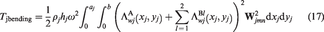
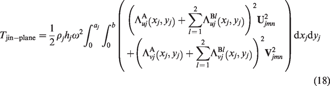
Based on the established model, this article is devoted to investigating the vibro-acoustic features of system, which consists of the L-shaped plate under any elastic BC and a cuboid acoustic cavity. The energy expression is got by using Rayleigh–Ritz energy method.^43–45 In the first place, the Lagrangian energy function of the L-shaped plate can be shown

$$L_{\text{plate}}=U_{\text{plate}}-T_{\text{plate}}-W_{\text{ext}}+W_{\text{a\&p}}$$

(15)

Here, T_plate is the entire kinetic energy

$$T_{\text{plane}}=T_{\text{1bending}}+T_{\text{1in-plane}}+T_{\text{2bending}}+T_{\text{2in-plane}}$$

(16)

where T_jbending and T_jin-plane represent, respectively, the j’th (j = 1,2) plate kinetic energy of bending and in-plane vibration. Take j’th plate as an example, potential energy and kinetic energy of different kinds of vibration can be expressed as

$$T_{\text{jbending}}=\frac{1}{2}{\rho }_j{h}_j{\omega }^2{\displaystyle {\int }_0^{a_j}{\displaystyle {\int }_0^b{\left({\mathbf{\Lambda }}_{\mathit{wj}}^{\text{A}}\left(x_j,y_j\right)+{\displaystyle \sum _{l\hspace{0.17em}=\hspace{0.17em}1}^2{\mathbf{\Lambda }}_{\mathit{wj}}^{\text{B}l}\left(x_j,y_j\right)}\right)}^2{\mathbf{W}}_{\mathit{jmn}}^2}}\text{d}{x}_j\text{d}{y}_j$$

(17)

$$T_{\text{jin-plane}}=\frac{1}{2}{\rho }_j{h}_j{\omega }^2{\displaystyle {\int }_0^{a_j}{\displaystyle {\int }_0^b}}\left(\begin{array}{l}{\left({\mathbf{\Lambda }}_{\mathit{uj}}^{\text{A}}\left(x_j,y_j\right)+{\displaystyle \sum _{l\hspace{0.17em}=\hspace{0.17em}1}^2{\mathbf{\Lambda }}_{\mathit{uj}}^{\text{B}l}\left(x_j,y_j\right)}\right)}^2{\mathbf{U}}_{\mathit{jmn}}^2\\ +{\left({\mathbf{\Lambda }}_{\mathit{vj}}^{\text{A}}\left(x_j,y_j\right)+{\displaystyle \sum _{l\hspace{0.17em}=\hspace{0.17em}1}^2{\mathbf{\Lambda }}_{\mathit{vj}}^{\text{B}l}\left(x_j,y_j\right)}\right)}^2{\mathbf{V}}_{\mathit{jmn}}^2\end{array}\right)\text{d}{x}_j\text{d}{y}_j$$

(18)

where ω is the circle frequency. The h_j and the ρ_j represent, respectively, thickness and mass density of the j’th (j = 1, 2) plate.

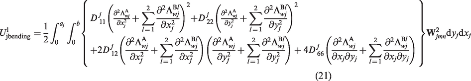
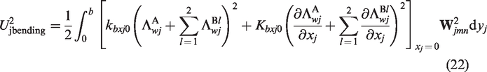
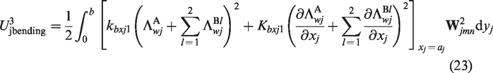
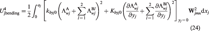
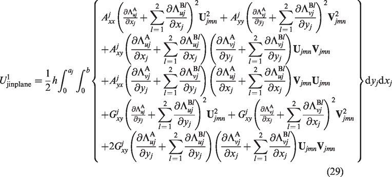
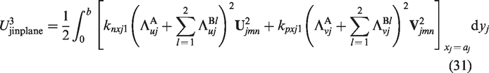
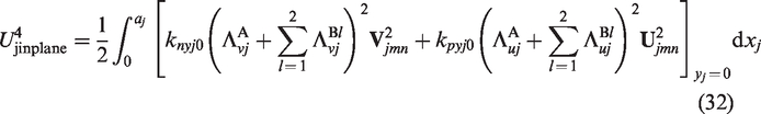
The entire potential energy is U_plate, and its expression can be written as

$$U_{\text{plate}}=U_{\text{1bending}}+U_{\text{1in-plane}}+U_{\text{2bending}}+U_{\text{2in-plane}}+U_{\text{coupling}}$$

(19)

where U_jbending (j = 1, 2) and U_jin-plane represent, respectively, the potential energy related with bending vibration and in-plane vibration in the j’th plate; U_coupling indicates the elastic potential energy laid in the coupling boundary spring. Take j’th plate as an example, potential energy and kinetic energy^46,47 can be expressed as

$$U_{\text{jbending}}=U_{\text{jbending}}^1\text{+}{U}_{\text{jbending}}^2\text{+}{U}_{\text{jbending}}^3\text{+}{U}_{\text{jbending}}^4\text{+}{U}_{\text{jbending}}^5$$

(20)

$$U_{\text{jbending}}^1=\frac{1}{2}{\displaystyle {\int }_0^{a_j}{\displaystyle {\int }_0^b}}\left\{\begin{array}{l}{D\hspace{0.17em}}_{11}^j{\left(\frac{{\partial }^2{\mathbf{\Lambda }}_{\mathit{wj}}^{\text{A}}}{\partial x_j^2}+{\displaystyle \sum _{l\hspace{0.17em}=\hspace{0.17em}1}^2\frac{{\partial }^2{\mathbf{\Lambda }}_{\mathit{wj}}^{\text{B}l}}{\partial x_j^2}}\right)}^2\text{+}{D\hspace{0.17em}}_{22}^j{\left(\frac{{\partial }^2{\mathbf{\Lambda }}_{\mathit{wj}}^{\text{A}}}{\partial y_j^2}+{\displaystyle \sum _{l\hspace{0.17em}=\hspace{0.17em}1}^2\frac{{\partial }^2{\mathbf{\Lambda }}_{\mathit{wj}}^{\text{B}l}}{\partial y_j^2}}\right)}^2\\ +2{D\hspace{0.17em}}_{12}^j\left(\frac{{\partial }^2{\mathbf{\Lambda }}_{\mathit{wj}}^{\text{A}}}{\partial x_j^2}+{\displaystyle \sum _{l\hspace{0.17em}=\hspace{0.17em}1}^2\frac{{\partial }^2{\mathbf{\Lambda }}_{\mathit{wj}}^{\text{B}l}}{\partial x_j^2}}\right)\left(\frac{{\partial }^2{\mathbf{\Lambda }}_{\mathit{wj}}^{\text{A}}}{\partial y_j^2}+{\displaystyle \sum _{l\hspace{0.17em}=\hspace{0.17em}1}^2\frac{{\partial }^2{\mathbf{\Lambda }}_{\mathit{wj}}^{\text{B}l}}{\partial y_j^2}}\right)+4{D\hspace{0.17em}}_{66}^j\left(\frac{{\partial }^2{\mathbf{\Lambda }}_{\mathit{wj}}^{\text{A}}}{\partial x_j\partial y_j}+{\displaystyle \sum _{l\hspace{0.17em}=\hspace{0.17em}1}^2\frac{{\partial }^2{\mathbf{\Lambda }}_{\mathit{wj}}^{\text{B}l}}{\partial x_j\partial y_j}}\right)\end{array}\right\}{\mathbf{W}}_{\mathit{jmn}}^2\text{d}{y}_j\text{d}{x}_j$$

(21)

$$U_{\text{jbending}}^2=\frac{1}{2}{{\displaystyle {\int }_0^b\left[k_{\mathit{bxj}0}{\left({\mathbf{\Lambda }}_{\mathit{wj}}^{\text{A}}+{\displaystyle \sum _{l\hspace{0.17em}=\hspace{0.17em}1}^2{\mathbf{\Lambda }}_{\mathit{wj}}^{\text{B}l}}\right)}^2+K_{\mathit{bxj}0}{\left(\frac{\partial {\mathbf{\Lambda }}_{\mathit{wj}}^{\text{A}}}{\partial x_j}+{\displaystyle \sum _{l\hspace{0.17em}=\hspace{0.17em}1}^2\frac{\partial {\mathbf{\Lambda }}_{\mathit{wj}}^{\text{B}l}}{\partial x_j}}\right)}^2\right]}}_{x_j\hspace{0.17em}=\hspace{0.17em}0}{\mathbf{W}}_{\mathit{jmn}}^2\text{d}{y}_j$$

(22)

$$U_{\text{jbending}}^3=\frac{1}{2}{{\displaystyle {\int }_0^b\left[k_{\mathit{bxj}1}{\left({\mathbf{\Lambda }}_{\mathit{wj}}^{\text{A}}+{\displaystyle \sum _{l\hspace{0.17em}=\hspace{0.17em}1}^2{\mathbf{\Lambda }}_{\mathit{wj}}^{\text{B}l}}\right)}^2+K_{\mathit{bxj}1}{\left(\frac{\partial {\mathbf{\Lambda }}_{\mathit{wj}}^{\text{A}}}{\partial x_j}+{\displaystyle \sum _{l\hspace{0.17em}=\hspace{0.17em}1}^2\frac{\partial {\mathbf{\Lambda }}_{\mathit{wj}}^{\text{B}l}}{\partial x_j}}\right)}^2\right]}}_{x_j\hspace{0.17em}=\hspace{0.17em}{a}_j}{\mathbf{W}}_{\mathit{jmn}}^2\text{d}{y}_j$$

(23)

$$U_{\text{jbending}}^4=\frac{1}{2}{{\displaystyle {\int }_0^{a_j}\left[k_{\mathit{byj}0}{\left({\mathbf{\Lambda }}_{\mathit{wj}}^{\text{A}}+{\displaystyle \sum _{l\hspace{0.17em}=\hspace{0.17em}1}^2{\mathbf{\Lambda }}_{\mathit{wj}}^{\text{B}l}}\right)}^2+K_{\mathit{byj}0}{\left(\frac{\partial {\mathbf{\Lambda }}_{\mathit{wj}}^{\text{A}}}{\partial y_j}+{\displaystyle \sum _{l\hspace{0.17em}=\hspace{0.17em}1}^2\frac{\partial {\mathbf{\Lambda }}_{\mathit{wj}}^{\text{B}l}}{\partial y_j}}\right)}^2\right]}}_{y_j\hspace{0.17em}=\hspace{0.17em}0}{\mathbf{W}}_{\mathit{jmn}}^2\text{d}{x}_j$$

(24)

$$U_{\text{jbending}}^5=\frac{1}{2}{{\displaystyle {\int }_0^{a_j}\left[k_{\mathit{byj}1}{\left({\mathbf{\Lambda }}_{\mathit{wj}}^{\text{A}}+{\displaystyle \sum _{l\hspace{0.17em}=\hspace{0.17em}1}^2{\mathbf{\Lambda }}_{\mathit{wj}}^{\text{B}l}}\right)}^2+K_{\mathit{byj}1}{\left(\frac{\partial {\mathbf{\Lambda }}_{\mathit{wj}}^{\text{A}}}{\partial y_j}+{\displaystyle \sum _{l\hspace{0.17em}=\hspace{0.17em}1}^2\frac{\partial {\mathbf{\Lambda }}_{\mathit{wj}}^{\text{B}l}}{\partial y_j}}\right)}^2\right]}}_{y_j\hspace{0.17em}=\hspace{0.17em}b}{\mathbf{W}}_{\mathit{jmn}}^2\text{d}{x}_j$$

(25)

where ${D\hspace{0.17em}}_{\mathit{xy}}^j$ are the bending rigidities and can be described as follows

$$\begin{array}{cccc}{D\hspace{0.17em}}_{11}^j=\frac{E_1^j{h}_j^3}{12\left(1-{\mu \hspace{0.17em}}_{12}^j{\mu \hspace{0.17em}}_{21}^j\right)}& {D\hspace{0.17em}}_{22}^j=\frac{E_2^j{h}_j^3}{12\left(1-{\mu \hspace{0.17em}}_{12}^j{\mu \hspace{0.17em}}_{21}^j\right)}& {D\hspace{0.17em}}_{12}^j={\mu \hspace{0.17em}}_{12}^j{D\hspace{0.17em}}_{22}^j& {D\hspace{0.17em}}_{66}^j=\frac{G_{12}^j{h}_j^3}{12}\end{array}$$

(26)

$E_1^j$ and $E_2^j$ denote the Young’s modulus in x-direction and y-direction of the j’th plate; $G_{12}^j$ is the shear modulus associated with x–y plane of the j’th plate; and ${\mu \hspace{0.17em}}_{12}^j$ and ${\mu \hspace{0.17em}}_{21}^j$ represent the major and minor Poisson’s ratio of the j’th plate. Due to four elastic constants, $E_1^j$ , $E_2^j$ , $G_{12}^j$ , and ${\mu \hspace{0.17em}}_{12}^j$ , are independent, the coefficient ${\mu \hspace{0.17em}}_{21}^j$ can be determined according to the following relation

$${\mu \hspace{0.17em}}_{12}^j{E}_2^j={\mu \hspace{0.17em}}_{21}^j{E}_1^j$$

(27)

$$U_{\text{jinplane}}=U_{\text{jinplane}}^1\text{+}{U}_{\text{jinplane}}^2\text{+}{U}_{\text{jinplane}}^3\text{+}{U}_{\text{jinplane}}^4\text{+}{U}_{\text{jinplane}}^5$$

(28)

$$U_{\text{jinplane}}^1=\frac{1}{2}h{\displaystyle {\int }_0^{a_j}{\displaystyle {\int }_0^b}}\left\{\begin{array}{l}{A}_{\mathit{xx}}^j{\left(\frac{\partial {\mathbf{\Lambda }}_{\mathit{uj}}^{\text{A}}}{\partial x_j}+{\displaystyle \sum _{l\hspace{0.17em}=\hspace{0.17em}1}^2\frac{\partial {\mathbf{\Lambda }}_{\mathit{uj}}^{\text{B}l}}{\partial x_j}}\right)}^2{\mathbf{U}}_{\mathit{jmn}}^2+A_{\mathit{yy}}^j{\left(\frac{\partial {\mathbf{\Lambda }}_{\mathit{vj}}^{\text{A}}}{\partial y_j}+{\displaystyle \sum _{l\hspace{0.17em}=\hspace{0.17em}1}^2\frac{\partial {\mathbf{\Lambda }}_{\mathit{vj}}^{\text{B}l}}{\partial y_j}}\right)}^2{\mathbf{V}}_{\mathit{jmn}}^2\\ +A_{\mathit{xy}}^j\left(\frac{\partial {\mathbf{\Lambda }}_{\mathit{uj}}^{\text{A}}}{\partial x_j}+{\displaystyle \sum _{l\hspace{0.17em}=\hspace{0.17em}1}^2\frac{\partial {\mathbf{\Lambda }}_{\mathit{uj}}^{\text{B}l}}{\partial x_j}}\right)\left(\frac{\partial {\mathbf{\Lambda }}_{\mathit{vj}}^{\text{A}}}{\partial y_j}+{\displaystyle \sum _{l\hspace{0.17em}=\hspace{0.17em}1}^2\frac{\partial {\mathbf{\Lambda }}_{\mathit{vj}}^{\text{B}l}}{\partial y_j}}\right){\mathbf{U}}_{\mathit{jmn}}{\mathbf{V}}_{\mathit{jmn}}\\ +A_{\mathit{yx}}^j\left(\frac{\partial {\mathbf{\Lambda }}_{\mathit{vj}}^{\text{A}}}{\partial y_j}+{\displaystyle \sum _{l\hspace{0.17em}=\hspace{0.17em}1}^2\frac{\partial {\mathbf{\Lambda }}_{\mathit{vj}}^{\text{B}l}}{\partial y_j}}\right)\left(\frac{\partial {\mathbf{\Lambda }}_{\mathit{uj}}^{\text{A}}}{\partial x_j}+{\displaystyle \sum _{l\hspace{0.17em}=\hspace{0.17em}1}^2\frac{\partial {\mathbf{\Lambda }}_{\mathit{uj}}^{\text{B}l}}{\partial x_j}}\right){\mathbf{V}}_{\mathit{jmn}}{\mathbf{U}}_{\mathit{jmn}}\\ +G_{\mathit{xy}}^j{\left(\frac{\partial {\mathbf{\Lambda }}_{\mathit{uj}}^{\text{A}}}{\partial y_j}+{\displaystyle \sum _{l\hspace{0.17em}=\hspace{0.17em}1}^2\frac{\partial {\mathbf{\Lambda }}_{\mathit{uj}}^{\text{B}l}}{\partial y_j}}\right)}^2{\mathbf{U}}_{\mathit{jmn}}^2+G_{\mathit{xy}}^j{\left(\frac{\partial {\mathbf{\Lambda }}_{\mathit{vj}}^{\text{A}}}{\partial x_j}+{\displaystyle \sum _{l\hspace{0.17em}=\hspace{0.17em}1}^2\frac{\partial {\mathbf{\Lambda }}_{\mathit{vj}}^{\text{B}l}}{\partial x_j}}\right)}^2{\mathbf{V}}_{\mathit{jmn}}^2\\ +2G_{\mathit{xy}}^j\left(\frac{\partial {\mathbf{\Lambda }}_{\mathit{uj}}^{\text{A}}}{\partial y_j}+{\displaystyle \sum _{l\hspace{0.17em}=\hspace{0.17em}1}^2\frac{\partial {\mathbf{\Lambda }}_{\mathit{uj}}^{\text{B}l}}{\partial y_j}}\right)\left(\frac{\partial {\mathbf{\Lambda }}_{\mathit{vj}}^{\text{A}}}{\partial x_j}+{\displaystyle \sum _{l\hspace{0.17em}=\hspace{0.17em}1}^2\frac{\partial {\mathbf{\Lambda }}_{\mathit{vj}}^{\text{B}l}}{\partial x_j}}\right){\mathbf{U}}_{\mathit{jmn}}{\mathbf{V}}_{\mathit{jmn}}\end{array}\right\}\text{d}{y}_j\text{d}{x}_j$$

(29)

$$U_{\text{jinplane}}^2=\frac{1}{2}{{\displaystyle {\int }_0^b\left[k_{\mathit{nxj}0}{\left({\mathbf{\Lambda }}_{\mathit{uj}}^{\text{A}}+{\displaystyle \sum _{l\hspace{0.17em}=\hspace{0.17em}1}^2{\mathbf{\Lambda }}_{\mathit{uj}}^{\text{B}l}}\right)}^2{\mathbf{U}}_{\mathit{jmn}}^2+k_{\mathit{pxj}0}{\left({\mathbf{\Lambda }}_{\mathit{vj}}^{\text{A}}+{\displaystyle \sum _{l\hspace{0.17em}=\hspace{0.17em}1}^2{\mathbf{\Lambda }}_{\mathit{vj}}^{\text{B}l}}\right)}^2{\mathbf{V}}_{\mathit{jmn}}^2\right]}}_{x_j\hspace{0.17em}=\hspace{0.17em}0}\text{d}{y}_j$$

(30)

$$U_{\text{jinplane}}^3=\frac{1}{2}{{\displaystyle {\int }_0^b\left[k_{\mathit{nxj}1}{\left({\mathbf{\Lambda }}_{\mathit{uj}}^{\text{A}}+{\displaystyle \sum _{l\hspace{0.17em}=\hspace{0.17em}1}^2{\mathbf{\Lambda }}_{\mathit{uj}}^{\text{B}l}}\right)}^2{\mathbf{U}}_{\mathit{jmn}}^2+k_{\mathit{pxj}1}{\left({\mathbf{\Lambda }}_{\mathit{vj}}^{\text{A}}+{\displaystyle \sum _{l\hspace{0.17em}=\hspace{0.17em}1}^2{\mathbf{\Lambda }}_{\mathit{vj}}^{\text{B}l}}\right)}^2{\mathbf{V}}_{\mathit{jmn}}^2\right]}}_{x_j\hspace{0.17em}=\hspace{0.17em}{a}_j}\text{d}{y}_j$$

(31)

$$U_{\text{jinplane}}^4=\frac{1}{2}{{\displaystyle {\int }_0^{a_j}\left[k_{\mathit{nyj}0}{\left({\mathbf{\Lambda }}_{\mathit{vj}}^{\text{A}}+{\displaystyle \sum _{l\hspace{0.17em}=\hspace{0.17em}1}^2{\mathbf{\Lambda }}_{\mathit{vj}}^{\text{B}l}}\right)}^2{\mathbf{V}}_{\mathit{jmn}}^2+k_{\mathit{pyj}0}{\left({\mathbf{\Lambda }}_{\mathit{uj}}^{\text{A}}+{\displaystyle \sum _{l\hspace{0.17em}=\hspace{0.17em}1}^2{\mathbf{\Lambda }}_{\mathit{uj}}^{\text{B}l}}\right)}^2{\mathbf{U}}_{\mathit{jmn}}^2\right]}}_{y_j\hspace{0.17em}=\hspace{0.17em}0}\text{d}{x}_j$$

(32)

$$U_{\text{jinplane}}^5=\frac{1}{2}{{\displaystyle {\int }_0^{a_j}\left[k_{\mathit{nyj}1}{\left({\mathbf{\Lambda }}_{\mathit{vj}}^{\text{A}}+{\displaystyle \sum _{l\hspace{0.17em}=\hspace{0.17em}1}^2{\mathbf{\Lambda }}_{\mathit{vj}}^{\text{B}l}}\right)}^2{\mathbf{V}}_{\mathit{jmn}}^2+k_{\mathit{pyj}1}{\left({\mathbf{\Lambda }}_{\mathit{uj}}^{\text{A}}+{\displaystyle \sum _{l\hspace{0.17em}=\hspace{0.17em}1}^2{\mathbf{\Lambda }}_{\mathit{uj}}^{\text{B}l}}\right)}^2{\mathbf{U}}_{\mathit{jmn}}^2\right]}}_{y_j\hspace{0.17em}=\hspace{0.17em}b}\text{d}{x}_j$$

(33)

$$\begin{array}{cccc}{A}_{\mathit{xx}}^j=\frac{E_1^j}{1-{\mu \hspace{0.17em}}_{\mathit{x}}^{\mathit{j}}{\mu \hspace{0.17em}}_{\mathit{y}}^{\mathit{j}}}& A_{\mathit{yy}}^j=\frac{E_2^j}{1-{\mu \hspace{0.17em}}_{\mathit{x}}^{\mathit{j}}{\mu \hspace{0.17em}}_{\mathit{y}}^{\mathit{j}}}& A_{\mathit{xy}}^j=\frac{{\mu \hspace{0.17em}}_{\mathit{x}}^{\mathit{j}}{E}_1^j}{1-{\mu \hspace{0.17em}}_{\mathit{x}}^{\mathit{j}}{\mu \hspace{0.17em}}_{\mathit{y}}^{\mathit{j}}}& A_{\mathit{xx}}^j=\frac{{\mu \hspace{0.17em}}_{\mathit{y}}^{\mathit{j}}{E}_1^j}{1-{\mu \hspace{0.17em}}_{\mathit{x}}^{\mathit{j}}{\mu \hspace{0.17em}}_{\mathit{y}}^{\mathit{j}}}\end{array}$$

(34)

where $A_{\mathit{xx}}^j$ , $A_{\mathit{yy}}^j$ , $A_{\mathit{xy}}^j$ , and $A_{\mathit{yx}}^j$ are the stretch stiffness, and $G_{12}^j$ is the shear stiffness. ${\mu \hspace{0.17em}}_{\mathit{s}}^{\mathit{j}}$ are the Poisson’s ration in x-direction and y-direction of the j’th plate. k_bxj0, k_bxj1, k_byj0, k_byj1, k_nxj0, k_nxj1, k_nyj0, k_nyj1, k_pxj0, k_pxj1, k_pyj0, and k_pyj1 are the linear springs located on the j’th plate and K_bxj0, K_bxj1, K_byj0, and K_byj1 are the rotational springs located on the j’th plate.

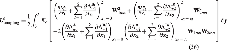
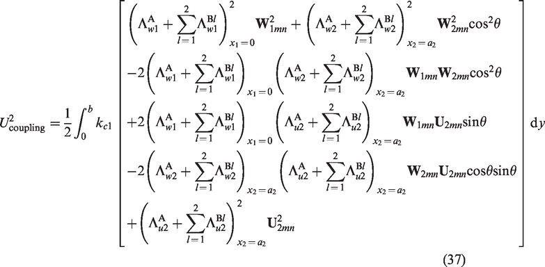
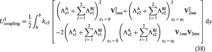
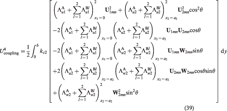
Because the coupling angle is non-zero, coupling relationship needs to be considered. This structural coupling can be described, and U_coupling is noted as representing the elastic potential energy stored in the coupling boundary spring.

$$U_{\text{coupling}}=U_{\text{coupling}}^1\text{+}{U}_{\text{coupling}}^2\text{+}{U}_{\text{coupling}}^3\text{+}{U}_{\text{coupling}}^4$$

(35)

$$U_{\text{coupling}}^1=\frac{1}{2}{\displaystyle {\int }_0^b{K}_c\left[\begin{array}{l}{\left(\frac{\partial {\mathbf{\Lambda }}_{w1}^{\text{A}}}{\partial x_1}+{\displaystyle \sum _{l\hspace{0.17em}=\hspace{0.17em}1}^2\frac{\partial {\mathbf{\Lambda }}_{w1}^{\text{B}l}}{\partial x_1}}\right)}_{x_1\hspace{0.17em}=\hspace{0.17em}0}^2{\mathbf{W}}_{1mn}^2+{\left(\frac{\partial {\mathbf{\Lambda }}_{w2}^{\text{A}}}{\partial x_2}+{\displaystyle \sum _{l\hspace{0.17em}=\hspace{0.17em}1}^2\frac{\partial {\mathbf{\Lambda }}_{w2}^{\text{B}l}}{\partial x_2}}\right)}_{x_2\hspace{0.17em}=\hspace{0.17em}{a}_2}^2{\mathbf{W}}_{2mn}^2\\ -2{\left(\frac{\partial {\mathbf{\Lambda }}_{w1}^{\text{A}}}{\partial x_1}+{\displaystyle \sum _{l\hspace{0.17em}=\hspace{0.17em}1}^2\frac{\partial {\mathbf{\Lambda }}_{w1}^{\text{B}l}}{\partial x_1}}\right)}_{x_1\hspace{0.17em}=\hspace{0.17em}0}{\left(\frac{\partial {\mathbf{\Lambda }}_{w2}^{\text{A}}}{\partial x_2}+{\displaystyle \sum _{l\hspace{0.17em}=\hspace{0.17em}1}^2\frac{\partial {\mathbf{\Lambda }}_{w2}^{\text{B}l}}{\partial x_2}}\right)}_{x_2\hspace{0.17em}=\hspace{0.17em}{a}_2}{\mathbf{W}}_{1mn}{\mathbf{W}}_{2mn}\end{array}\right]}\text{d}y$$

(36)

$$U_{\text{coupling}}^2=\frac{1}{2}{\displaystyle {\int }_0^b{k}_{c1}\left[\begin{array}{l}{\left({\mathbf{\Lambda }}_{w1}^{\text{A}}+{\displaystyle \sum _{l\hspace{0.17em}=\hspace{0.17em}1}^2{\mathbf{\Lambda }}_{w1}^{\text{B}l}}\right)}_{x_1\hspace{0.17em}=\hspace{0.17em}0}^2{\mathbf{W}}_{1mn}^2+{\left({\mathbf{\Lambda }}_{w2}^{\text{A}}+{\displaystyle \sum _{l\hspace{0.17em}=\hspace{0.17em}1}^2{\mathbf{\Lambda }}_{w2}^{\text{B}l}}\right)}_{x_2\hspace{0.17em}=\hspace{0.17em}{a}_2}^2{\mathbf{W}}_{2mn}^2{\cos }^2\theta \\ -2{\left({\mathbf{\Lambda }}_{w1}^{\text{A}}+{\displaystyle \sum _{l\hspace{0.17em}=\hspace{0.17em}1}^2{\mathbf{\Lambda }}_{w1}^{\text{B}l}}\right)}_{x_1\hspace{0.17em}=\hspace{0.17em}0}{\left({\mathbf{\Lambda }}_{w2}^{\text{A}}+{\displaystyle \sum _{l\hspace{0.17em}=\hspace{0.17em}1}^2{\mathbf{\Lambda }}_{w2}^{\text{B}l}}\right)}_{x_2\hspace{0.17em}=\hspace{0.17em}{a}_2}{\mathbf{W}}_{1mn}{\mathbf{W}}_{2mn}{\cos }^2\theta \\ +2{\left({\mathbf{\Lambda }}_{w1}^{\text{A}}+{\displaystyle \sum _{l\hspace{0.17em}=\hspace{0.17em}1}^2{\mathbf{\Lambda }}_{w1}^{\text{B}l}}\right)}_{x_1\hspace{0.17em}=\hspace{0.17em}0}{\left({\mathbf{\Lambda }}_{u2}^{\text{A}}+{\displaystyle \sum _{l\hspace{0.17em}=\hspace{0.17em}1}^2{\mathbf{\Lambda }}_{u2}^{\text{B}l}}\right)}_{x_2\hspace{0.17em}=\hspace{0.17em}{a}_2}{\mathbf{W}}_{1mn}{\mathbf{U}}_{2mn}\sin \theta \\ -2{\left({\mathbf{\Lambda }}_{w2}^{\text{A}}+{\displaystyle \sum _{l\hspace{0.17em}=\hspace{0.17em}1}^2{\mathbf{\Lambda }}_{w2}^{\text{B}l}}\right)}_{x_2\hspace{0.17em}=\hspace{0.17em}{a}_2}{\left({\mathbf{\Lambda }}_{u2}^{\text{A}}+{\displaystyle \sum _{l\hspace{0.17em}=\hspace{0.17em}1}^2{\mathbf{\Lambda }}_{u2}^{\text{B}l}}\right)}_{x_2\hspace{0.17em}=\hspace{0.17em}{a}_2}{\mathbf{W}}_{2mn}{\mathbf{U}}_{2mn}\cos \theta \sin \theta \\ +{\left({\mathbf{\Lambda }}_{u2}^{\text{A}}+{\displaystyle \sum _{l\hspace{0.17em}=\hspace{0.17em}1}^2{\mathbf{\Lambda }}_{u2}^{\text{B}l}}\right)}_{x_2\hspace{0.17em}=\hspace{0.17em}{a}_2}^2{\mathbf{U}}_{2mn}^2\end{array}\right]}\text{d}y$$

(37)

$$U_{\text{coupling}}^3=\frac{1}{2}{\displaystyle {\int }_0^b{k}_{c3}\left[\begin{array}{l}{\left({\mathbf{\Lambda }}_{v1}^{\text{A}}+{\displaystyle \sum _{l\hspace{0.17em}=\hspace{0.17em}1}^2{\mathbf{\Lambda }}_{v1}^{\text{B}l}}\right)}_{x_1\hspace{0.17em}=\hspace{0.17em}0}^2{\mathbf{V}}_{1mn}^2\text{+}{\left({\mathbf{\Lambda }}_{v2}^{\text{A}}+{\displaystyle \sum _{l\hspace{0.17em}=\hspace{0.17em}1}^2{\mathbf{\Lambda }}_{v2}^{\text{B}l}}\right)}_{x_2\hspace{0.17em}=\hspace{0.17em}{a}_2}^2{\mathbf{V}}_{2mn}^2\\ -2{\left({\mathbf{\Lambda }}_{v1}^{\text{A}}+{\displaystyle \sum _{l\hspace{0.17em}=\hspace{0.17em}1}^2{\mathbf{\Lambda }}_{v1}^{\text{B}l}}\right)}_{x_1\hspace{0.17em}=\hspace{0.17em}0}{\left({\mathbf{\Lambda }}_{v2}^{\text{A}}+{\displaystyle \sum _{l\hspace{0.17em}=\hspace{0.17em}1}^2{\mathbf{\Lambda }}_{v2}^{\text{B}l}}\right)}_{x_2\hspace{0.17em}=\hspace{0.17em}{a}_2}{\mathbf{V}}_{1mn}{\mathbf{V}}_{2mn}\end{array}\right]}\text{d}y$$

(38)

$$U_{\text{coupling}}^4=\frac{1}{2}{\displaystyle {\int }_0^b{k}_{c2}\left[\begin{array}{l}{\left({\mathbf{\Lambda }}_{u1}^{\text{A}}+{\displaystyle \sum _{l\hspace{0.17em}=\hspace{0.17em}1}^2{\mathbf{\Lambda }}_{u1}^{\text{B}l}}\right)}_{x_1\hspace{0.17em}=\hspace{0.17em}0}^2{\mathbf{U}}_{1mn}^2+{\left({\mathbf{\Lambda }}_{u2}^{\text{A}}+{\displaystyle \sum _{l\hspace{0.17em}=\hspace{0.17em}1}^2{\mathbf{\Lambda }}_{u2}^{\text{B}l}}\right)}_{x_2\hspace{0.17em}=\hspace{0.17em}{a}_2}^2{\mathbf{U}}_{2mn}^2{\cos }^2\theta \\ -2{\left({\mathbf{\Lambda }}_{u1}^{\text{A}}+{\displaystyle \sum _{l\hspace{0.17em}=\hspace{0.17em}1}^2{\mathbf{\Lambda }}_{u1}^{\text{B}l}}\right)}_{x_1\hspace{0.17em}=\hspace{0.17em}0}{\left({\mathbf{\Lambda }}_{u2}^{\text{A}}+{\displaystyle \sum _{l\hspace{0.17em}=\hspace{0.17em}1}^2{\mathbf{\Lambda }}_{u2}^{\text{B}l}}\right)}_{x_2\hspace{0.17em}=\hspace{0.17em}{a}_2}{\mathbf{U}}_{1mn}{\mathbf{U}}_{2mn}\cos \theta \\ -2{\left({\mathbf{\Lambda }}_{u1}^{\text{A}}+{\displaystyle \sum _{l\hspace{0.17em}=\hspace{0.17em}1}^2{\mathbf{\Lambda }}_{u1}^{\text{B}l}}\right)}_{x_1\hspace{0.17em}=\hspace{0.17em}0}{\left({\mathbf{\Lambda }}_{w2}^{\text{A}}+{\displaystyle \sum _{l\hspace{0.17em}=\hspace{0.17em}1}^2{\mathbf{\Lambda }}_{w2}^{\text{B}l}}\right)}_{x_2\hspace{0.17em}=\hspace{0.17em}{a}_2}{\mathbf{U}}_{1mn}{\mathbf{W}}_{2mn}\sin \theta \\ \text{+}2{\left({\mathbf{\Lambda }}_{u2}^{\text{A}}+{\displaystyle \sum _{l\hspace{0.17em}=\hspace{0.17em}1}^2{\mathbf{\Lambda }}_{u2}^{\text{B}l}}\right)}_{x_2\hspace{0.17em}=\hspace{0.17em}{a}_2}{\left({\mathbf{\Lambda }}_{w2}^{\text{A}}+{\displaystyle \sum _{l\hspace{0.17em}=\hspace{0.17em}1}^2{\mathbf{\Lambda }}_{w2}^{\text{B}l}}\right)}_{x_2\hspace{0.17em}=\hspace{0.17em}{a}_2}{\mathbf{U}}_{2mn}{\mathbf{W}}_{2mn}\cos \theta \sin \theta \\ \text{+}{\left({\mathbf{\Lambda }}_{w2}^{\text{A}}+{\displaystyle \sum _{l\hspace{0.17em}=\hspace{0.17em}1}^2{\mathbf{\Lambda }}_{w2}^{\text{B}l}}\right)}_{x_2\hspace{0.17em}=\hspace{0.17em}{a}_2}^2{\mathbf{W}}_{2mn}^2{\sin }^2\theta \end{array}\right]}\text{d}y$$

(39)

where θ is the coupling angle. K_c, k_c1, k_c2, and k_c3 represent the stiffness coefficients of the four coupling springs. k_c1, k_c2, and k_c3 are the linear springs. Besides, K_c is the rotational springs.

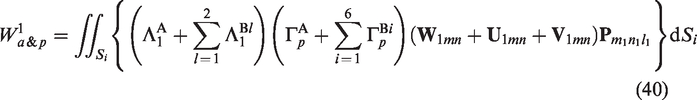
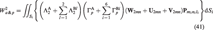
In the plate–cavity coupling system, the plate–cavity coupling interface needs to satisfy the particle vibration velocity continuity condition. For the continuity equations that need to be satisfied at the internal interface of the structure–acoustic coupling system, the mutual work between the structure and the sound field will be described in the energy principle analysis framework. W_a&p shows that the sound pressure on the coupling surface does work on the plate. It can be expressed as

$$W_{a\hspace{0.17em}\&\hspace{0.17em}p}^1={\displaystyle {\iint }_{S_i}\left\{\left({\mathbf{\Lambda }}_1^{\text{A}}+{\displaystyle \sum _{l\hspace{0.17em}=\hspace{0.17em}1}^2{\mathbf{\Lambda }}_1^{\text{B}l}}\right)\left({\mathbf{\Gamma }}_p^{\text{A}}+{\displaystyle \sum _{i\hspace{0.17em}=\hspace{0.17em}1}^6{\mathbf{\Gamma }}_p^{\text{B}i}}\right)\left({\mathbf{W}}_{1mn}+{\mathbf{U}}_{1mn}+{\mathbf{V}}_{1mn}\right){\mathbf{P}}_{m_1{n}_1{l}_1}\right\}}\text{d}{S}_i$$

(40)

$$W_{a\hspace{0.17em}\&\hspace{0.17em}p}^2={\displaystyle {\iint }_{S_i}\left\{\left({\mathbf{\Lambda }}_2^{\text{A}}+{\displaystyle \sum _{l\hspace{0.17em}=\hspace{0.17em}1}^2{\mathbf{\Lambda }}_2^{\text{B}l}}\right)\left({\mathbf{\Gamma }}_p^{\text{A}}+{\displaystyle \sum _{i\hspace{0.17em}=\hspace{0.17em}1}^6{\mathbf{\Gamma }}_p^{\text{B}i}}\right)\left({\mathbf{W}}_{2mn}+{\mathbf{U}}_{2mn}+{\mathbf{V}}_{2mn}\right){\mathbf{P}}_{m_1{n}_1{l}_1}\right\}}\text{d}{S}_i$$

(41)

in which S_i shows the associated surface between the L-shaped plate and the cuboid cavity. W_ext represents the work done.

$$W_{\text{ext}}={\displaystyle {\iint }_S\left\{\left({\mathbf{\Lambda }}^{\text{A}}+{\displaystyle \sum _{l\hspace{0.17em}=\hspace{0.17em}1}^2{\mathbf{\Lambda }}^{\text{B}l}}\right){\displaystyle \sum _{l\hspace{0.17em}=\hspace{0.17em}1}^2\left(f_{\mathit{wj}}{\mathbf{W}}_{\mathit{jmn}}+f_{\mathit{uj}}{\mathbf{U}}_{\mathit{jmn}}+f_{\mathit{vj}}{\mathbf{V}}_{\mathit{jmn}}\right)}\right\}}\text{d}{x}_j\text{d}{y}_j$$

(42)

in which f_i (i = u_j, v_j, and w_j) is the function of the external load distribution.

$$f_i=F_i\delta \left(x-x_0\right)\delta \left(y-y_0\right)$$

(43)

where δ is the Dirac function. x₀ and y₀ expresses the position where the external point force is applied.

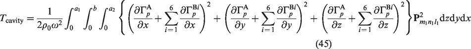
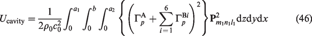
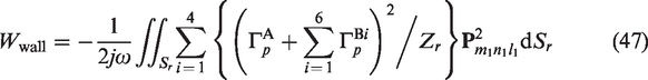
The Lagrangian energy function L_cavity for the cuboid cavity is supplied as

$$L_{\text{cavity}}=U_{\text{cavity}}-T_{\text{cavity}}-W_{\text{p\&a}}-W_{\text{wall}}-W_{\text{pss}}$$

(44)

in which the whole kinetic energy, the whole cuboid acoustic energy, and the dissipated cuboid acoustic energy are marked as U_cavity, T_cavity, and W_wall. Moreover, W_pss is the work done in cuboid acoustic cavity by point sound source.

$$T_{\text{cavity}}=\frac{1}{2{\rho }_0{\omega }^2}{\displaystyle {\int }_0^{a_1}{\displaystyle {\int }_0^b{\displaystyle {\int }_0^{a_2}\left\{{\left(\frac{\partial {\mathbf{\Gamma }}_p^{\text{A}}}{\partial x}+{\displaystyle \sum _{i\hspace{0.17em}=\hspace{0.17em}1}^6\frac{\partial {\mathbf{\Gamma }}_p^{\text{B}i}}{\partial x}}\right)}^2+{\left(\frac{\partial {\mathbf{\Gamma }}_p^{\text{A}}}{\partial y}+{\displaystyle \sum _{i\hspace{0.17em}=\hspace{0.17em}1}^6\frac{\partial {\mathbf{\Gamma }}_p^{\text{B}i}}{\partial y}}\right)}^2+{\left(\frac{\partial {\mathbf{\Gamma }}_p^{\text{A}}}{\partial z}+{\displaystyle \sum _{i\hspace{0.17em}=\hspace{0.17em}1}^6\frac{\partial {\mathbf{\Gamma }}_p^{\text{B}i}}{\partial z}}\right)}^2\right\}{\mathbf{P}}_{m_1{n}_1{l}_1}^2}}}\text{d}z\text{d}y\text{d}x$$

(45)

$$U_{\text{cavity}}=\frac{1}{2{\rho }_0{c}_0^2}{\displaystyle {\int }_0^{a_1}{\displaystyle {\int }_0^b{\displaystyle {\int }_0^{a_2}\left\{{\left({\mathbf{\Gamma }}_p^{\text{A}}+{\displaystyle \sum _{i\hspace{0.17em}=\hspace{0.17em}1}^6{\mathbf{\Gamma }}_p^{\text{B}i}}\right)}^2\right\}{\mathbf{P}}_{m_1{n}_1{l}_1}^2}}}\text{d}z\text{d}y\text{d}x$$

(46)

$$W_{\text{wall}}=-\frac{1}{2j\omega }{\displaystyle {\iint }_{S_r}{\displaystyle \sum _{i\hspace{0.17em}=\hspace{0.17em}1}^4\left\{{\left({\mathbf{\Gamma }}_p^{\text{A}}+{\displaystyle \sum _{i\hspace{0.17em}=\hspace{0.17em}1}^6{\mathbf{\Gamma }}_p^{\text{B}i}}\right)}^2/Z_r\right\}{\mathbf{P}}_{m_1{n}_1{l}_1}^2}}\text{d}{S}_r$$

(47)

$$W_{\text{pss}}\text{=}-\frac{1}{j\omega }{\displaystyle {\int }_0^{a_1}{\displaystyle {\int }_0^b{\displaystyle {\int }_0^{a_2}\left({\mathbf{\Gamma }}_p^{\text{A}}+{\displaystyle \sum _{i\hspace{0.17em}=\hspace{0.17em}1}^6{\mathbf{\Gamma }}_p^{\text{B}i}}\right)Q}}}{\mathbf{P}}_{m_1{n}_1{l}_1}\text{d}z\text{d}y\text{d}x$$

(48)

$$Q=\frac{4\pi A}{j{\rho }_0{c}_{0}k}\delta \left(x-x_e\right)\delta \left(y-y_e\right)\delta \left(z-z_e\right)$$

(49)

where S_r (r = 1, 2, 3, 4) represents the r’th non-related surface, and Z_r (r = 1, 2, 3, 4) shows the impedance on the r’th surface. In addition, A (in kg/s²) is the magnitude of Q.

Solution process of the structural–acoustic coupling system

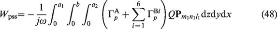
We can get by the solving equation of L-shaped plate and cuboid cavity coupling system by using the equations (15) and (49) based on the Rayleigh–Ritz energy method. ⁴⁸ The specific method is as follows

$$\frac{\partial L_{\text{plate}}}{\partial {\mathbf{H}}_{\mathit{mn}}}=\frac{\partial U_{\text{plate}}}{\partial {\mathbf{H}}_{\mathit{mn}}}-\frac{\partial T_{\text{plate}}}{\partial {\mathbf{H}}_{\mathit{mn}}}-\frac{\partial W_{\text{ext}}}{\partial {\mathbf{H}}_{\mathit{mn}}}+\frac{\partial W_{\text{a\&p}}}{\partial {\mathbf{H}}_{\mathit{mn}}}=0$$

(50)

$$\frac{\partial L_{\text{cavity}}}{\partial {\mathbf{P}}_{m_1{n}_1{l}_1}}=\frac{\partial U_{\text{cavity}}}{\partial {\mathbf{P}}_{m_1{n}_1{l}_1}}-\frac{\partial T_{\text{cavity}}}{\partial {\mathbf{P}}_{m_1{n}_1{l}_1}}-\frac{\partial W_{\text{p\&a}}}{\partial {\mathbf{P}}_{m_1{n}_1{l}_1}}-\frac{\partial W_{\text{wall}}}{\partial {\mathbf{P}}_{m_1{n}_1{l}_1}}-\frac{\partial W_{\text{pss}}}{\partial {\mathbf{P}}_{m_1{n}_1{l}_1}}=0$$

(51)

where $H_{\mathit{mn}}={\left[\begin{array}{cccccc}{\mathbf{W}}_{1mn}& {\mathbf{U}}_{1mn}& {\mathbf{V}}_{1mn}& {\mathbf{W}}_{2mn}& {\mathbf{U}}_{2mn}& {\mathbf{V}}_{2mn}\end{array}\right]}^{\text{T}}$ . Through taking equations (16) to (43) and (45) to (49) into equations (50) and (51), the equation can be written as the following formula

$$\left({\mathbf{K}}_{\text{plate}}-{\omega }^2{\mathbf{M}}_{\text{plate}}\right){\mathbf{H}}_{\mathit{mn}}+{\mathbf{C}}_{\text{a\&p}}{\mathbf{P}}_{m_1{n}_1{l}_1}={\mathbf{F}}_i$$

(52)

$$\left({\mathbf{K}}_{\text{cavity}}-\omega {\mathbf{Z}}_{\text{cavity}}-{\omega }^2{\mathbf{M}}_{\text{cavity}}\right){\mathbf{P}}_{m_1{n}_1{l}_1}+{\omega }^2{\mathbf{C}}_{\text{p\&a}}{\mathbf{H}}_{\mathit{mn}}=\mathbf{Q}$$

(53)

in which the stiffness matrix of L-shaped plate and cuboid cavity is noted as K_plate and K_cavity. The mass matrix of L-shaped plate and cuboid cavity is recorded as M_plate and M_cavity. C_a&p and C_p & a are the coupled matrix of the L-shaped plate and the cuboid cavity. ${\mathbf{C}}_{\text{p\hspace{0.17em}\&\hspace{0.17em}a}}={\mathbf{C}}_{\text{a\hspace{0.17em}\&\hspace{0.17em}p}}^{\text{T}}$ . The damping matrix is noted as Z_cavity.

In order to solve eigenvalue problem easily, we can convert the matrix to the following matrix

$$\left(\mathbf{K}-\omega \mathbf{M}\right)\mathbf{G}=0$$

(54)

$$\mathbf{K}=\left[\begin{array}{cccc}0& {\mathbf{K}}_{\text{plate}}& 0& 0\\ {\mathbf{K}}_{\text{plate}}& 0& {\mathbf{C}}_{\text{a\&p}}& 0\\ 0& 0& 0& {\mathbf{K}}_{\text{cavity}}\\ 0& 0& {\mathbf{K}}_{\text{cavity}}& \text{-}{\mathbf{Z}}_{\text{cavity}}\end{array}\right]$$

(55)

$$\mathbf{M}=\left[\begin{array}{cccc}{\mathbf{K}}_{\text{plate}}& 0& 0& 0\\ 0& {\mathbf{M}}_{\text{plate}}& 0& 0\\ 0& 0& {\mathbf{K}}_{\text{cavity}}& 0\\ 0& \text{-}{\mathbf{C}}_{\text{a\&p}}^{\text{T}}& 0& {\mathbf{M}}_{\text{cavity}}\end{array}\right]$$

(56)

$$\mathbf{G}={\left[\begin{array}{cccc}{\mathbf{H}}_{\mathit{mn}}& \omega {\mathbf{H}}_{\mathit{mn}}& {\mathbf{P}}_{m_1{n}_1{l}_1}& \omega {\mathbf{P}}_{m_1{n}_1{l}_1}\end{array}\right]}^{\text{T}}$$

(57)

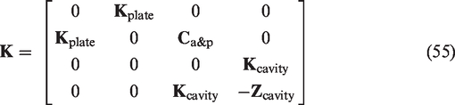
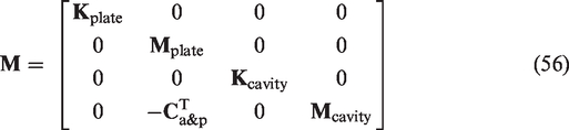
The simple matrix described above is more conducive to solving unknowns.

Numerical results and discussions

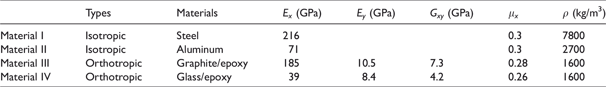
In order to study the natural features and forced responses, several numerical examples will be carried out in this section. The influence of impedance of the cuboid acoustic cavity and materials of the L-shaped plate on the coupling system is exploited importantly. Regarding the effects of the plate thickness, BC, and orthotropic degrees for the coupling system, we will summarize some new conclusions. Since some parameters in the article are repeated, some statements will be given here for the convenience of the following narrative. The mass density is ρ_air=1.21 kg/m³, and the sound speed in air is c_air=344 m/s in all the following numerical cases. The BC of L-shaped plate are described by alphabetic strings. Specifically, F, S, C, and E ⁱ (i = 1, 2) indicate that BC are free, simple, fixed, and elastic. For the elastic boundary, the E¹ elastic boundary is between free and simple, and the E² elastic boundary is between the simple and the fixed. This selection principle fully considers the BC of each stage. The order of the BC is y = 0, x = a₁, y = b, and x = 0 in plate 1. The boundary situations of the plate 2 are the same as those of the plate 1. The BC of E¹ means that all linear spring values are set to 0 N/m, and all rotational spring stiffness values are set to 1E3 Nm/rad. When all linear and rotational spring stiffness values are 1E6 N/m and 1E6 Nm/rad, respectively, the BC of E² will form. In Table 1, we list four types of material properties.

Table 1.

Four different types of material properties used in this paper.

	Types	Materials	Ex (GPa)	Ey (GPa)	Gxy (GPa)	μx	ρ (kg/m3)
Material I	Isotropic	Steel	216			0.3	7800
Material II	Isotropic	Aluminum	71			0.3	2700
Material III	Orthotropic	Graphite/epoxy	185	10.5	7.3	0.28	1600
Material IV	Orthotropic	Glass/epoxy	39	8.4	4.2	0.26	1600

Natural characteristics analysis of the L-shaped plate–cavity coupling system

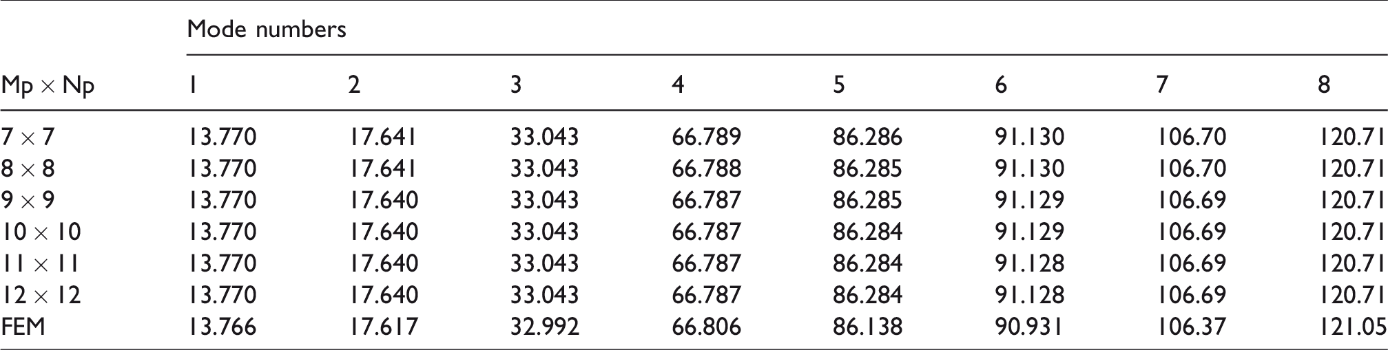
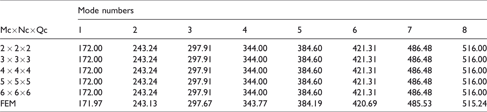
First of all, in order to guarantee the correctness of present method, evaluating its convergence and accuracy is necessary. Convergence degree of the L-shaped plate–cavity coupling system is made known by the cutoff value, which are represented by Mp and Np and Mc, Nc, and Qc. The convergence degree analysis is given in Tables 2 to 4. Compared with the results of FEM, the results got by this method are very consistent. The dimension symbols are the same as those shown in Figure 1. a₁ = 1 m, b = 1 m, a₂ = 1 m, and h₁ = h₂ = 0.008 m. As shown in Table 2, material of the L-shaped plate is Material I. And the BC are the coupled-edge fixed branches and the uncoupled edges free supported. The six faces of the cuboid acoustic cavity are rigid faces in Table 3. In Table 4, the materials and BC of the L-shaped coupled plate are the same as Table 2, and the non-coupling surfaces of the cuboid acoustic cavity are rigid surfaces. From Table 4, the convergence and accuracy of the L-shaped plate and a cuboid cavity coupling model directly are examined. It can be found that the coupling frequencies calculated based on different cutoff values have fluctuation phenomenon. However, the maximum fluctuation range is controlled within 0.5%, which can fully satisfy the convergence requirements. In addition, the Table 4 gives the comparative data calculated by the FEM. The maximum error of the results obtained by the method and the FEM is not more than 0.9%, which fully proves the correctness of the vibration characteristics analysis model of L-shaped plate–cavity coupling system established in this paper. In order to fully satisfy the convergence and accuracy, Mc = Nc = Qc = 3 and Mp = Np = 9 are selected as the cutoff values in the following numerical examples.

Table 2.

Convergence and accuracy of the first eight frequency f (Hz) for the L-shaped plate.

Mp × Np	Mode numbers
	1	2	3	4	5	6	7	8
7 × 7	13.770	17.641	33.043	66.789	86.286	91.130	106.70	120.71
8 × 8	13.770	17.641	33.043	66.788	86.285	91.130	106.70	120.71
9 × 9	13.770	17.640	33.043	66.787	86.285	91.129	106.69	120.71
10 × 10	13.770	17.640	33.043	66.787	86.284	91.129	106.69	120.71
11 × 11	13.770	17.640	33.043	66.787	86.284	91.128	106.69	120.71
12 × 12	13.770	17.640	33.043	66.787	86.284	91.128	106.69	120.71
FEM	13.766	17.617	32.992	66.806	86.138	90.931	106.37	121.05

Table 3.

Convergence and accuracy of natural frequencies f (Hz) for the rigid-walled acoustic cavity.

Mc×Nc×Qc	Mode numbers
	1	2	3	4	5	6	7	8
2 × 2×2	172.00	243.24	297.91	344.00	384.60	421.31	486.48	516.00
3 × 3×3	172.00	243.24	297.91	344.00	384.60	421.31	486.48	516.00
4 × 4×4	172.00	243.24	297.91	344.00	384.60	421.31	486.48	516.00
5 × 5×5	172.00	243.24	297.91	344.00	384.60	421.31	486.48	516.00
6 × 6×6	172.00	243.24	297.91	344.00	384.60	421.31	486.48	516.00
FEM	171.97	243.13	297.67	343.77	384.19	420.69	485.53	515.24

Table 4.

Convergence and accuracy of natural frequencies f (Hz) for the L-shaped plate–cavity coupling system.

Mc×Nc×Qc	Mp×Np	Mode numbers
		1	3	5	7	9	11
3 × 3×3	8 × 8	13.616	17.505	32.724	66.337	85.495	89.842
	9 × 9	13.616	17.505	32.724	66.336	85.495	89.836
	10 × 10	13.616	17.506	32.730	66.335	85.404	89.842
	11 × 11	13.616	17.505	32.724	66.336	85.500	89.842
	12 × 12	13.616	17.505	32.724	66.336	85.486	89.836
4 × 4×4	8 × 8	13.616	17.505	32.724	66.337	85.494	89.846
	9 × 9	13.616	17.504	32.723	66.328	85.491	89.885
	10 × 10	13.616	17.512	32.726	66.357	85.511	89.842
	11 × 11	13.615	17.529	32.749	66.342	85.234	89.842
	12 × 12	13.617	17.502	32.727	66.334	85.488	89.821
5 × 5×5	8 × 8	13.616	17.505	32.702	66.336	85.491	89.836
	9 × 9	13.616	17.515	32.721	66.353	85.496	89.845
	10 × 10	13.616	17.506	32.723	66.353	85.494	89.832
	11 × 11	13.616	17.505	32.722	66.322	85.497	89.832
	12 × 12	13.616	17.505	32.726	66.333	85.496	89.842
FEM		13.496	17.401	32.756	66.475	85.372	89.898

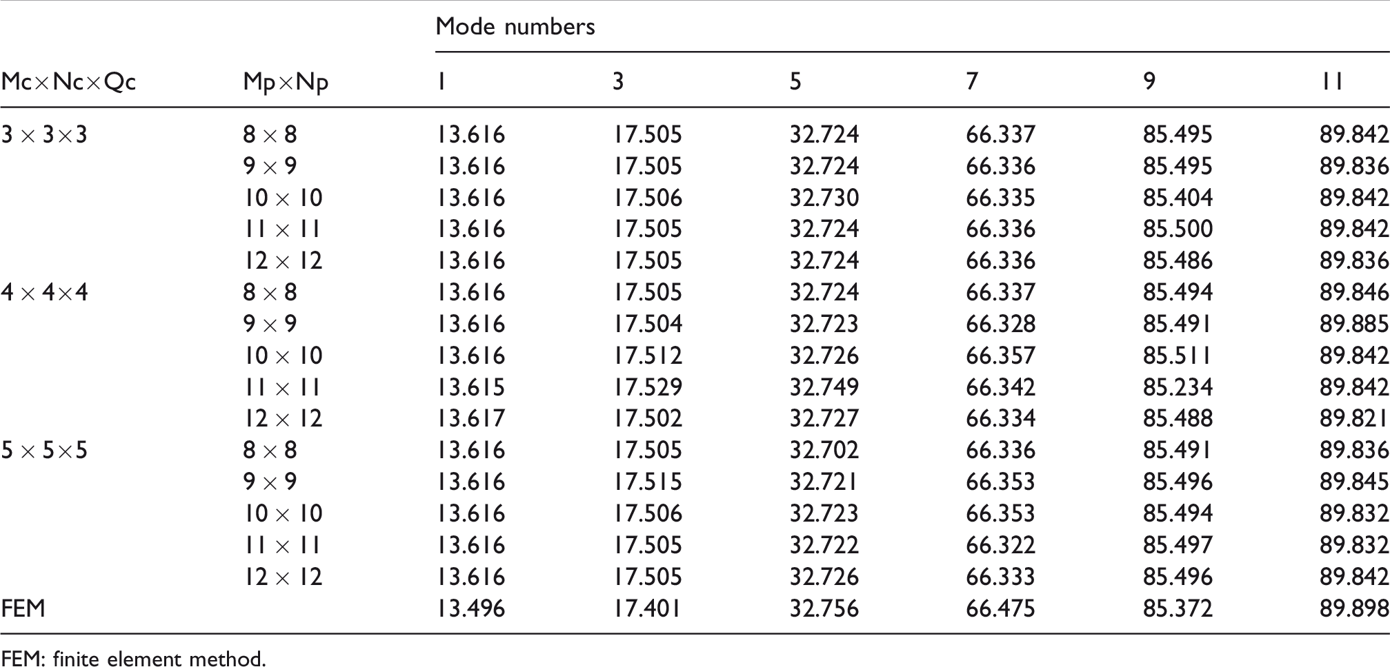
FEM: finite element method.

In order to deepen the intuitive understanding of the vibration characteristics of orthotropic L-shaped plate–cavity coupling system, the displacement mode shapes of the L-shaped plate are given in Figure 2, as well as the corresponding acoustic pressure mode shapes of the acoustic cavity. The dimension symbols are the same as those shown in Figure 1. a₁ = 1 m, b = 1 m, a₂ = 1 m, and h₁ = h₂ = 0.008 m. Material of the L-shaped plate is Material III. The BC are all fixed branches. From the mode shapes, we can directly see the displacement distribution of the L-shaped plate and the sound pressure distribution of the acoustic cavity at the natural frequencies. The mode shapes provide the basis for the analysis of the vibration characteristics of the structural system.

Figure 2.

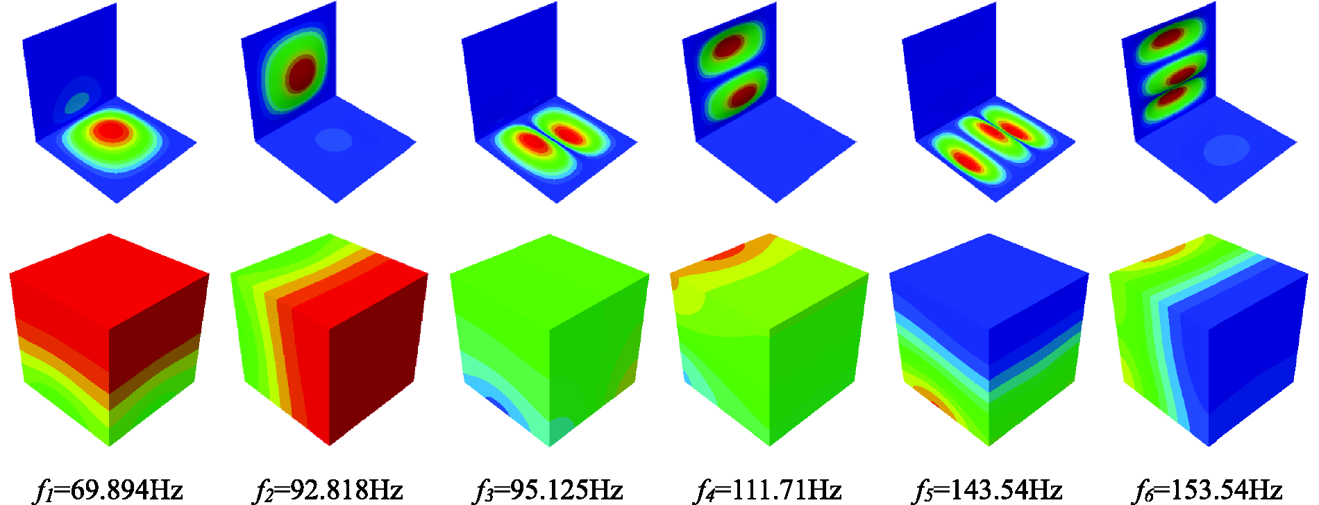
The mode shapes and natural frequency f (Hz) of the L-shaped plate–cavity coupling system.

Then we probe the coupling theory of the coupled system by Table 5. The degrees of change in the natural frequencies can be expressed by ratios, and the degrees of coupling can be visually displayed. The ratios is δ = coupled natural frequencies/structural natural frequencies = CNF/SNF. The sizes of the cuboid acoustic cavity are a₁×b×a₂ = 1.4 m × 1.0 m × 1.2 m. Remaining walls are all rigid, all but the L-shaped plate surface for the cuboid acoustic cavity. The thickness of the L-shaped plate with classic (F, S, and C) and elastic BC is h₁ = h₂ = 0.008 m and materials I and III are used in table. Typically, the CNF are slightly less than the SNF, but all the ratios are exceedingly close to 1. Moreover, the BC have a great impact on the CNF and SNF. It is obvious which frequencies of the structural and the coupled increase as the increase of stiffness value. It is worthy to mention that no matter which stiffness value we chose, it does not change which all the ratios are exceedingly close to 1.

Table 5.

The natural frequencies f (Hz) and coupling degrees of the L-shaped plate–cavity coupling system filled with air.

Precondition	BC	Mode numbers	SNF		CNF		δ
			Present	FEM	Present	FEM	Present	FEM
Material I	FFFC	3	9.932	9.876	9.892	9.8932	0.9959	1.0017
		4	15.208	15.080	15.297	15.099	1.0058	1.0012
		5	22.098	22.181	22.287	22.400	1.0085	1.0098
		6	34.876	34.772	34.781	34.833	0.9972	1.0017
	SSSC	3	63.564	63.971	63.270	63.696	0.9957	0.9957
		4	67.457	67.867	67.250	67.619	0.9969	0.9963
		5	80.605	81.056	80.359	80.715	0.9969	0.9957
		6	102.52	103.09	102.20	102.76	0.9968	0.9967
	CCCC	3	81.018	81.576	80.784	81.053	0.9971	0.9935
		4	97.595	98.282	97.313	97.893	0.9975	0.9960
		5	112.07	112.80	111.81	112.23	0.9976	0.9949
		6	131.74	132.63	131.20	132.05	0.9959	0.9956
Material III	FFFC	3	13.771	13.767	16.349	16.283	1.1872	1.1827
		4	16.552	16.535	19.918	19.993	1.2033	1.2091
		5	20.517	20.498	20.341	20.334	0.9914	0.9919
		6	27.028	26.986	26.838	26.761	0.9929	0.9916
	SSSC	3	62.604	62.495	62.525	62.313	0.9987	0.9970
		4	72.249	72.086	71.011	71.090	0.9828	0.9861
		5	72.878	72.909	72.207	72.484	0.9907	0.9941
		6	94.975	94.837	93.814	94.018	0.9877	0.9913
	CCCC	3	90.499	90.243	88.952	88.798	0.9829	0.9856
		4	96.914	97.054	95.779	96.463	0.9882	0.9939
		5	102.03	101.76	99.698	100.39	0.9771	0.9865
		6	126.34	125.98	117.63	118.89	0.9310	0.9416

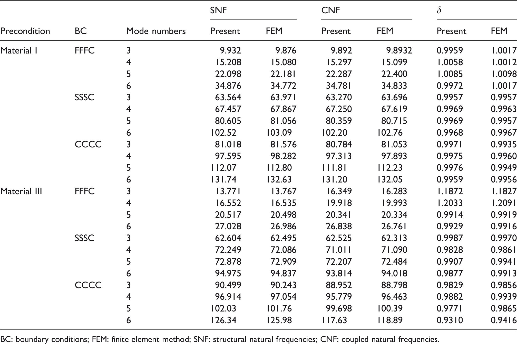
BC: boundary conditions; FEM: finite element method; SNF: structural natural frequencies; CNF: coupled natural frequencies.

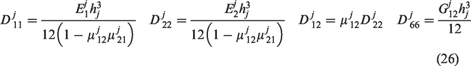
To further check the versatility and accuracy of the present method, the natural frequencies of the L-shaped plate-cavity coupling model with different materials and BC are given (Table 6). Four materials are used in Table 6, including two isotropic materials and two orthotropic materials. In the use of the formula, the property parameters of isotropic materials are special cases of the property parameters of isotropic materials. The specific changes are as follows E₁ = E₂, G₁₂ = E₁/(2 + 2μ₁₂). Therefore, the properties of Material I are given as E₁ = E₂ = 216 GPa, G₁₂ = 83.1 GPa, μ₁₂ = 0.3, and ρ = 7800 kg/m³. The geometrical parameters of the cavity are a₁×b×a₂ = 1.4 m × 1.2 m × 1.0 m, and the geometrical parameters of the plate are a₁×b×h₁ = 1.4 m × 1.2 m × 0.008 m and a₂×b×h₂ = 1.0 m × 1.2 m × 0.008 m. Except the coupling surface, other walls are acoustically rigid. At the end of the table, the natural frequencies of elastic BC are also given. It is easy to know that the results received by this method are consistent with the results got by FEM. From the data given in Table 6, we can come to a conclusion that the more fixed BC, the higher the natural frequencies of the L-shaped plate and cuboid cavity coupling model.

Table 6.

The natural frequencies f (Hz) of the L-shaped plate–cavity coupling system with different materials and boundary conditions (h₁ = h₂ = 0.008 m).

Precondition	BC	Method	Mode numbers
			3	4	5	6	7	8
Material I	FFFC	Present	9.892	15.297	22.287	34.781	35.926	39.551
		FEM	9.893	15.099	22.400	34.833	35.985	39.476
	CCCC	Present	80.784	97.313	111.81	131.20	139.39	140.96
		FEM	81.053	97.893	112.23	132.05	140.33	140.33
Material II	SFSF	Present	19.986	24.942	41.272	52.361	53.184	60.934
		FEM	20.011	24.817	41.116	52.490	52.857	60.838
	FCFF	Present	13.456	14.664	22.427	33.754	34.891	38.369
		FEM	13.322	14.602	22.467	33.684	34.854	38.258
Material III	SSSS	Present	42.747	53.456	67.393	79.671	80.435	90.644
		FEM	42.616	53.391	67.637	79.888	80.637	90.989
	CCCS	Present	64.017	78.061	89.913	100.20	108.45	114.20
		FEM	63.905	78.314	90.522	101.03	108.85	115.12
Material IV	SCSC	Present	44.021	52.557	59.357	61.699	70.027	75.487
		FEM	43.729	52.257	59.254	61.620	69.854	75.113
	FSFC	Present	30.080	30.984	39.045	45.774	46.583	48.619
		FEM	29.902	30.992	38.835	45.725	46.475	48.538
Material I	E1E1E1E1	Present	18.156	27.285	27.415	39.671	49.109	70.411
	E2E2E2E2	Present	72.930	94.461	98.912	99.218	117.14	118.32
Material III	E1E1E1E1	Present	18.317	21.272	42.652	53.414	57.697	79.319
	E2E2E2E2	Present	61.556	64.803	76.726	78.576	99.446	102.91

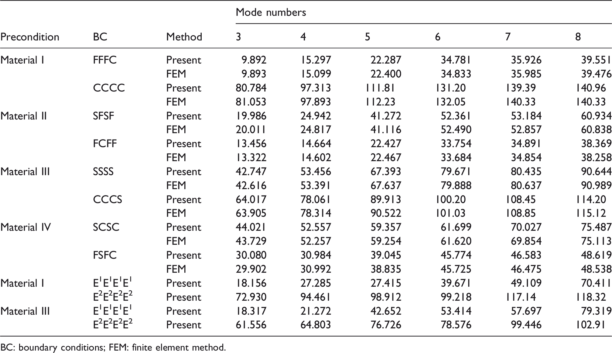
BC: boundary conditions; FEM: finite element method.

As shown in Table 7, we mainly analyze effects of different thickness ratios. The sizes of the cuboid acoustic cavity are a₁×b×a₂ = 1.4 m × 1.0 m × 1.2 m. Except the L-shaped coupling surface for the cuboid acoustic cavity, other four walls are all rigid. The thickness of L-shaped plate 1 with simple BC is h₁ = 0.008 m and Material III is used in Table 7. It can be summarized from the table that when the thickness of the two plates is different, as the thickness ratio of the two plates increases, the natural frequency increases.

Table 7.

The natural frequencies f (Hz) of the L-shaped plate–cavity coupling system with various plate thicknesses (Material III, SSSS, h₁ = 0.001 m).

Thickness h2/h1	Methods	Mode numbers
		3	4	5	6	7	8	9	10
0.125	Present	1.567	1.896	2.292	2.395	2.718	2.819	3.468	4.357
	FEM	1.366	2.272	2.674	2.789	2.933	3.070	3.674	4.852
0.25	Present	2.632	3.438	3.753	4.339	4.533	5.089	5.159	6.143
	FEM	2.732	2.933	4.545	4.957	5.348	5.578	6.141	7.349
0.5	Present	4.526	4.584	7.271	7.937	8.081	9.192	10.175	10.740
	FEM	3.483	4.957	5.465	9.090	9.569	10.696	10.777	11.156
1	Present	6.446	7.694	9.082	9.777	10.669	13.206	13.552	15.078
	FEM	6.172	7.813	9.151	9.452	10.714	13.407	13.608	14.765
2	Present	13.146	15.899	19.211	19.668	22.154	27.199	27.871	30.371
	FEM	12.892	15.963	19.220	19.326	22.166	27.278	27.876	30.039
4	Present	26.644	27.970	34.760	39.544	40.710	45.160	55.158	56.525
	FEM	26.388	28.221	34.739	39.519	40.595	45.126	55.173	56.467
8	Present	42.747	53.456	67.393	79.671	80.435	90.644	110.59	112.80
	FEM	42.616	53.391	67.637	79.888	80.637	90.989	111.36	113.40

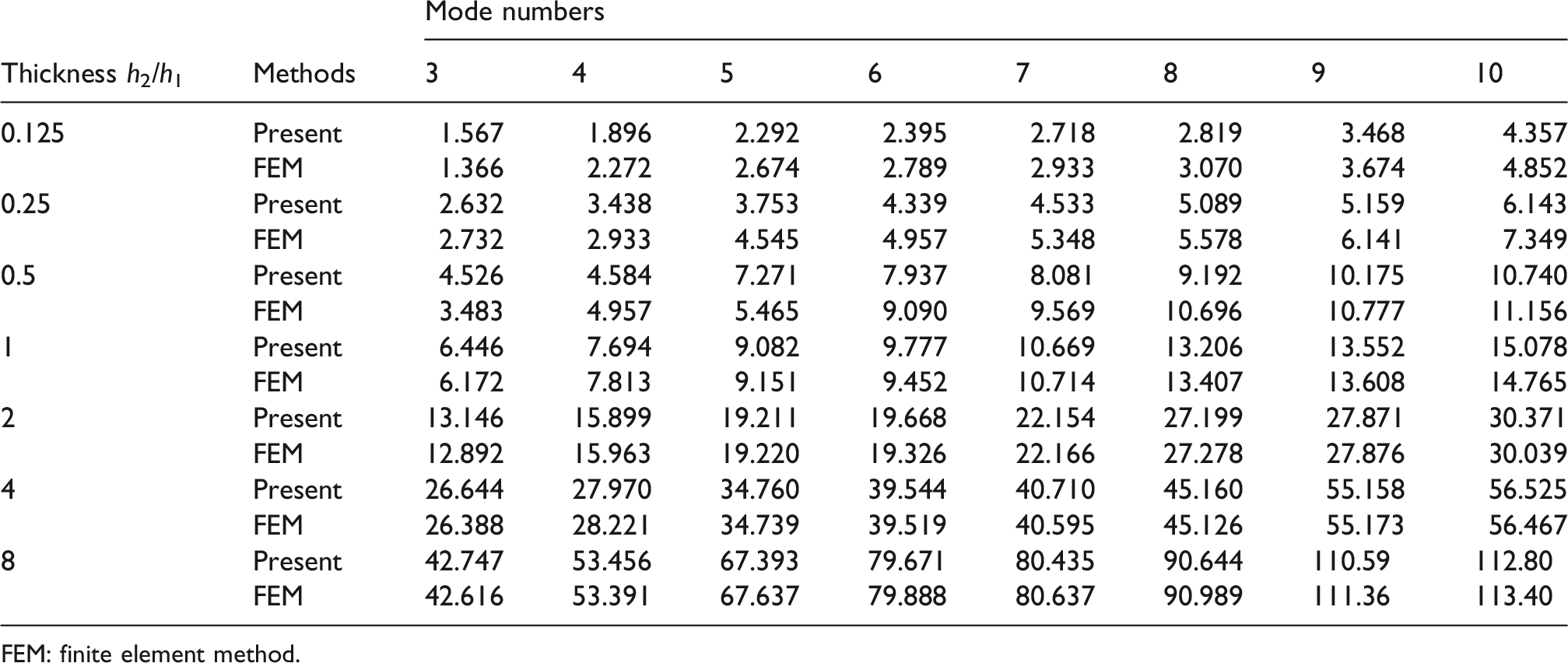
FEM: finite element method.

For the orthotropic L-shaped plate–cavity coupling system, an important factor is orthotropic degree. The influence of different orthotropic degrees and BC on the natural frequencies is shown in Table 8. The sizes used in Table 8 are same as Table 6. And related property parameters are as follows: E₂ = 10 GPa, G₁₂ = 5 GPa, μ₁₂ = 0.25, and ρ = 1300 kg/m³. The non-related surfaces are rigid walls. At the end of the table, the natural frequencies of two groups of elastic BC are also given. The natural frequencies are different under any BC and several orthotropic degrees from Table 8. Specifically, with increasing the spring stiffness value and the anisotropic degree, the natural frequencies will increase. In the case where the BC are the same, the natural frequency increases as the orthotropic degrees increases. It has important value of engineering guidance. By picking a group of different BC and orthotropic degrees, the frequencies which have a good match for specific requirements can be utilized.

Table 8.

The natural frequencies f (Hz) of the L-shaped plate–cavity coupling system with varying boundary conditions and orthotropic degrees (h₁ = h₂ = 0.008 m, E₂ = 10 GPa, G₁₂ = 5 GPa, μ₁₂ = 0.25, and ρ = 1300 kg/m³).

BC	E1/E2	Methods	Mode numbers
			3	4	5	6	7	8	9
FFFF	10	Present	15.553	15.841	25.367	32.029	36.421	41.081	43.308
		FEM	15.642	15.696	25.306	31.839	36.409	41.039	43.334
	20	Present	15.552	15.839	25.472	32.132	43.106	43.658	51.429
		FEM	15.641	15.695	25.408	31.938	43.276	43.356	51.391
	40	Present	15.551	15.838	25.548	32.203	43.113	43.661	52.825
		FEM	15.640	15.694	25.481	32.004	43.283	43.359	52.718
SSSS	10	Present	37.408	49.514	66.689	70.552	79.358	80.691	105.78
		FEM	37.236	49.125	66.602	70.458	79.153	80.160	105.52
	20	Present	48.662	58.610	72.275	86.570	91.510	101.90	119.19
		FEM	48.231	58.157	72.174	85.944	91.406	101.58	119.06
	40	Present	65.801	73.500	75.726	97.367	118.33	121.26	134.02
		FEM	64.908	72.881	75.614	96.582	119.76	121.09	134.23
CCCC	10	Present	60.705	75.699	89.349	98.350	102.43	118.16	120.77
		FEM	60.637	74.714	88.708	98.267	102.36	117.33	118.98
	20	Present	103.87	104.86	114.05	121.47	140.45	144.85	145.71
		FEM	100.95	104.67	112.80	123.67	139.93	143.83	145.18
	40	Present	116.73	122.33	141.92	143.62	154.72	164.82	170.94
		FEM	116.31	119.99	141.05	145.74	152.43	164.27	171.30
CSCS	10	Present	74.159	78.950	82.010	101.10	105.02	111.73	123.98
		FEM	73.088	78.844	81.340	100.83	104.29	111.31	123.80
	20	Present	86.913	102.65	108.27	121.21	127.03	129.10	144.94
		FEM	86.683	99.699	107.07	122.45	127.83	128.83	144.30
	40	Present	100.99	122.38	137.59	142.35	142.67	152.16	161.99
		FEM	100.52	119.58	137.14	140.88	145.36	150.65	160.52
CFCF	10	Present	45.127	65.422	72.501	72.655	79.331	95.609	98.625
		FEM	45.024	65.267	71.383	72.042	78.829	95.039	98.472
	20	Present	57.996	74.950	101.38	101.44	106.83	108.70	119.60
		FEM	57.790	74.694	98.187	100.09	105.85	108.38	118.52
	40	Present	77.555	91.073	120.38	122.45	137.96	141.55	147.10
		FEM	77.053	90.498	119.04	119.83	135.82	144.80	145.39
E1E1E1E1	10	Present	16.234	16.554	25.931	32.565	36.759	41.439	43.579
	20	Present	16.231	16.550	26.042	32.672	43.365	43.922	51.674
	40	Present	16.229	16.549	26.121	32.743	43.371	43.923	53.119
E2E2E2E2	10	Present	44.140	52.867	54.605	56.895	60.645	71.834	77.030
	20	Present	51.674	55.454	60.822	67.688	84.967	85.768	91.336
	40	Present	54.606	60.954	72.848	75.635	85.992	94.068	102.11

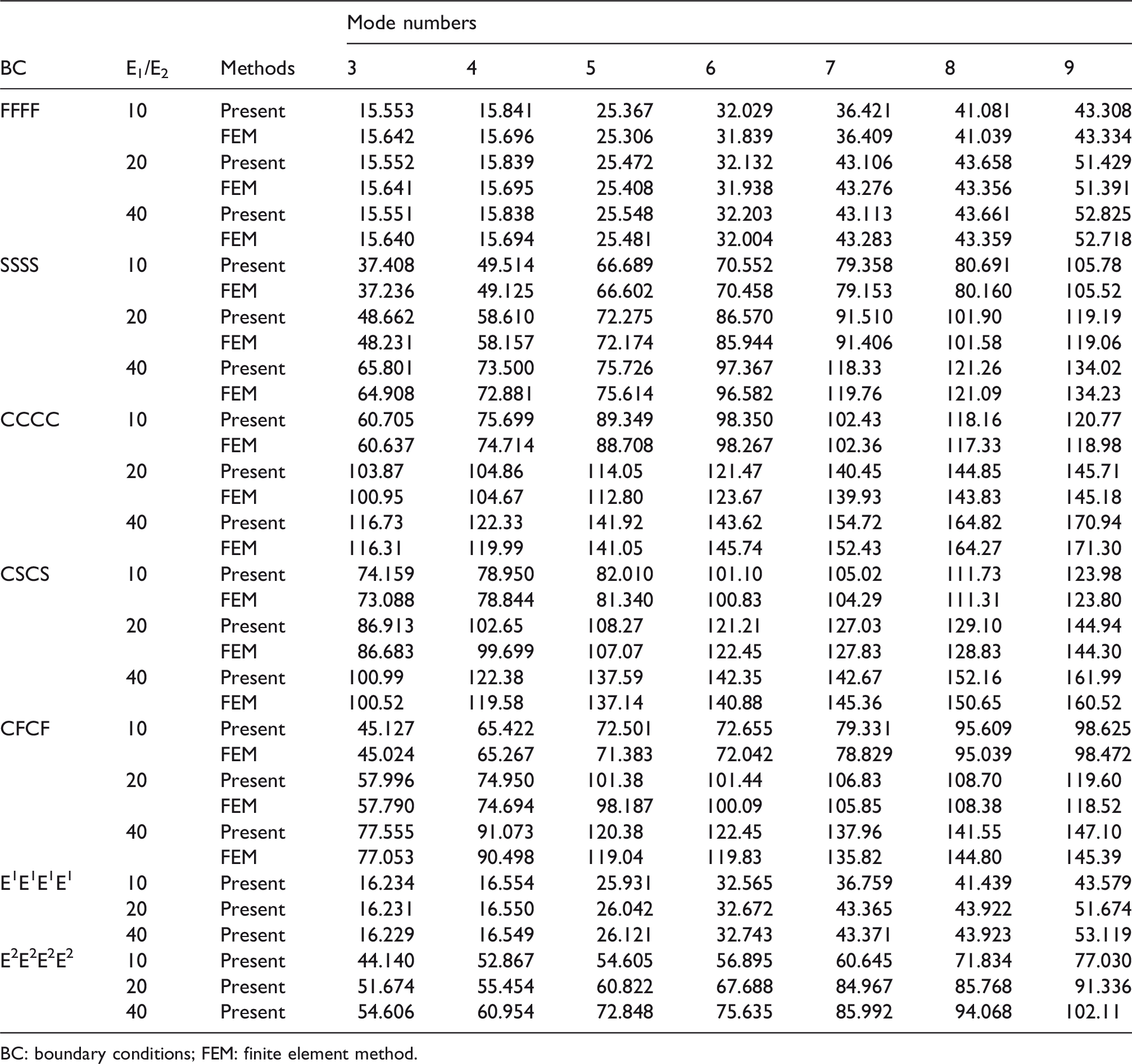
BC: boundary conditions; FEM: finite element method.

In fact, there are also cases where two plates use different materials, so the relationship of the materials of the L-shaped plate on the natural frequencies is shown in Figure 3. The dimensions and BC are the same as those shown in Table 4. In the first picture, the influence of isotropic materials is mainly investigated. It can be seen that the change of isotropic materials has little influence on the natural frequencies. In the second picture, it is obtained that the connection of the orthotropic materials for the natural frequencies. From the figure, it can safely come to conclusion that the change of orthotropic materials has a tremendous influence on the natural frequencies. More specifically, when the materials of the plate 1 and the plate 2 are different, the natural frequencies are between the natural frequencies of the same material used separately. The third picture studies the natural frequencies of both isotropic and orthotropic materials. All these data clearly prove the fact that the natural frequencies in the presence of isotropic and orthotropic materials are mainly affected by orthotropic materials. We can choose the materials of the two plates to obtain the natural characteristics that meet the concrete requirements.

Figure 3.

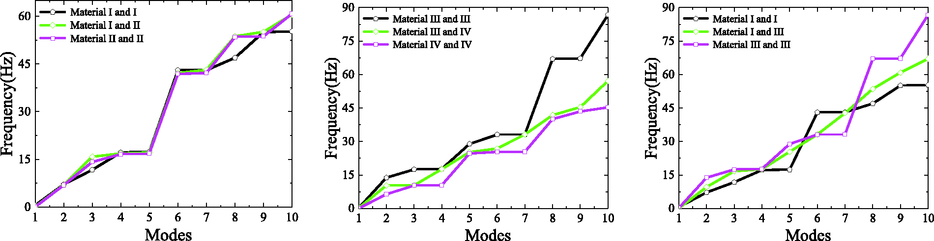
The natural frequency f (Hz) of the L-shaped plate–cavity coupling system under different materials of two plates.

Displacement and sound pressure analysis of the L-shaped plate–cavity coupling system

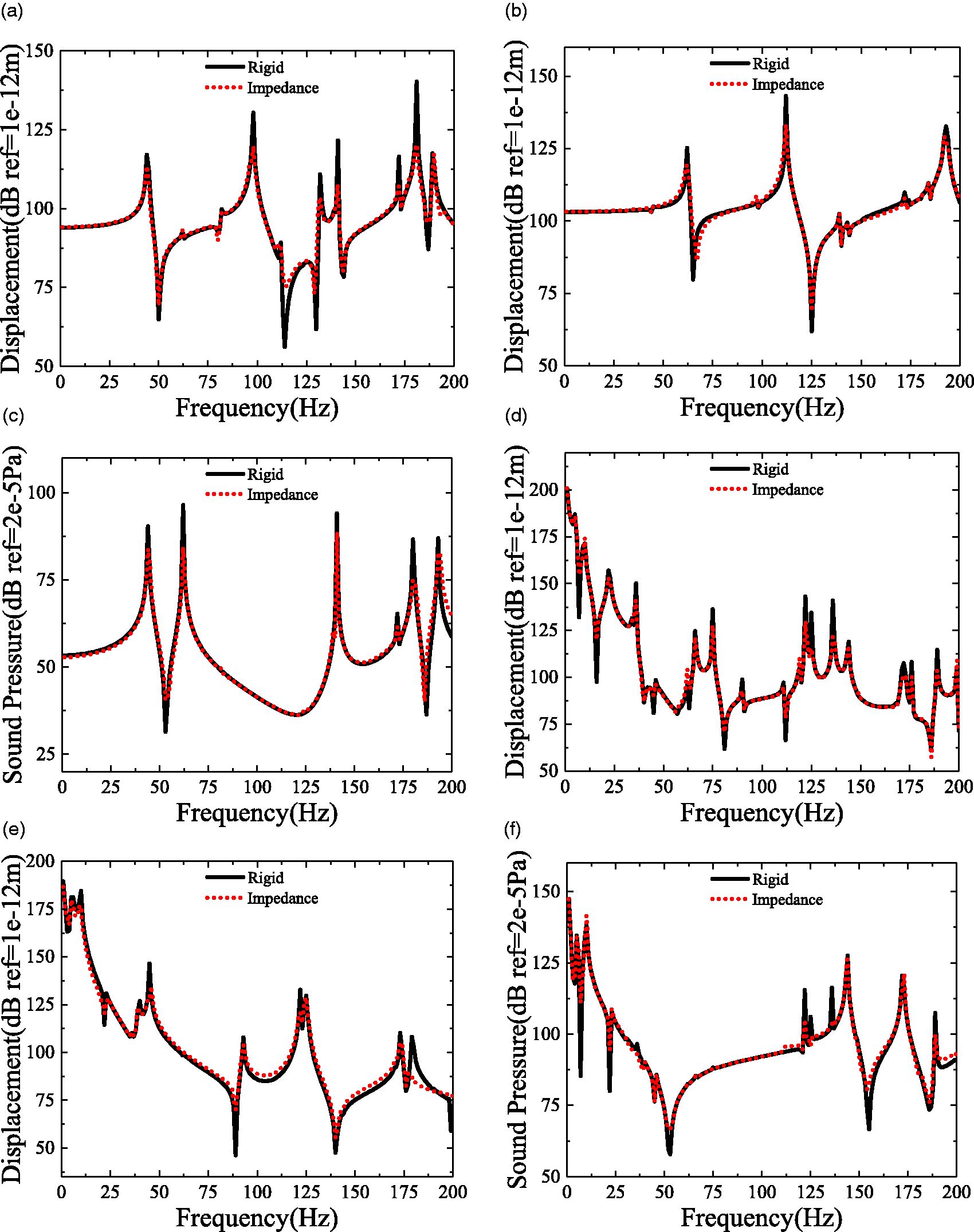
Forced response of L-shaped plate–cavity coupled system is analyzed in this part. First at all, Figure 4 shows the displacement and sound pressure response of the L-shaped plate and cuboid cavity model under the action of point force. The sizes of the L-shaped plate used in Figure 4 are a₁ = 1.4 m, a₂ = 1.0 m, b = 1.2 m, and h₁ = h₂ = 0.008 m. The isotropic material in the figure is selected from Material I. The orthotropic material is selected from the Material III. The BC of the coupled boundary shown in the figure are fixed. And the remaining boundaries situations are fixed and free, respectively. The boundary situations named in the figure represent only the BC of non-coupled boundary. The L-shaped plate is forced to two forces. The unit point force is applied to point (0.65,0.15) of plate 1 and point (0.65,0.15) of plate 2. In this figure, two points on the plate 1 and the plate 2 are selected to study displacement response analysis, and sound pressure responses analysis also are performed. Obviously, comparing the responses of different materials under different boundary situations, it can be deduced which BC cause deviation of the response curve, because the change of the spring value with the simulated BC changes the inherent of the coupled system. By comparing the results of this paper with the results of the FEM, the results of the present method can be obtained with good consistency.

Figure 4.

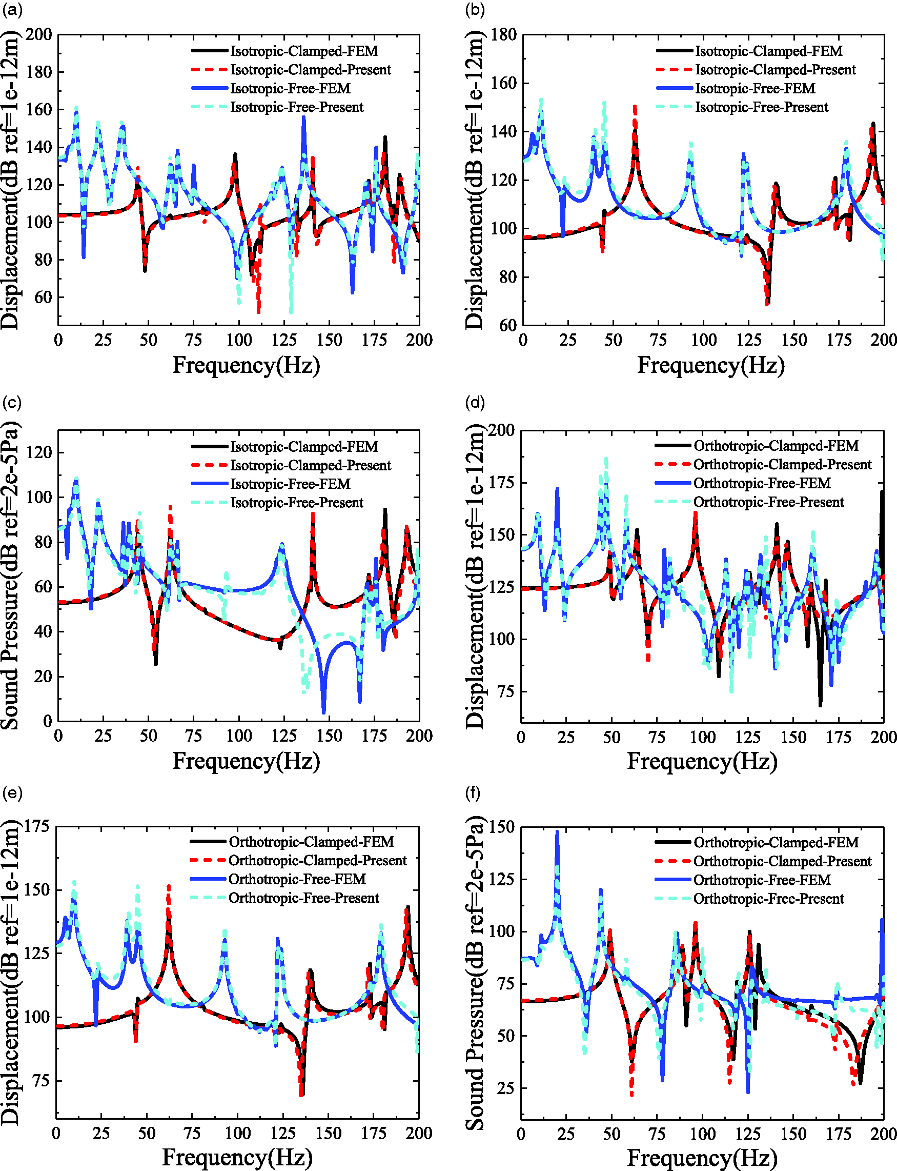
Responses of the L-shaped plate–cavity coupling system filled with air under the excitation of point forces (F₁ and F₂). (a) Displacement at (0.65,0.15) in plate 1. (b) Displacement at (0.5,0.6) in plate 2. (c) Sound Pressure at (0.7,0.6,0.5). (d) Displacement at (0.65,0.15) in plate 1. (e) Displacement at (0.5,0.6) in plate 2. (f) Sound Pressure at (0.7,0.6,0.5).

Next, we discuss the coupling mechanism between the coupled systems. In order to understand the forced response research under the action of point forces, we select the plate structure and coupled system. The Figure 5 explains the displacement value of the L-shaped plate and L-shaped plate–cavity system under the excitation of point forces. Here, materials of the L-shaped coupled structure are selected as the Material I (Figure 5(a) and (b)) and Material III (Figure 5(c) and (d)). And the boundary situations of the L-shaped structure are full clamped support. The dimensions are same as those of Figure 4. It can be known from the figure that the trend of the displacement curve is generally consistent. The displacement at the natural frequency is slightly offset. And the ratio of the displacement value of the L-shaped plate and the L-shaped plate–cavity model at the peak is close to 1. It can be seen from the figure that the displacement of plate under the coupling system is smaller than the displacement before the coupling, indicating that the displacement has a weakening effect before and after the coupling. When using the orthotropic materials, the displacement response is also affected at the local frequency due to the presence of the cuboid cavity.

Figure 5.

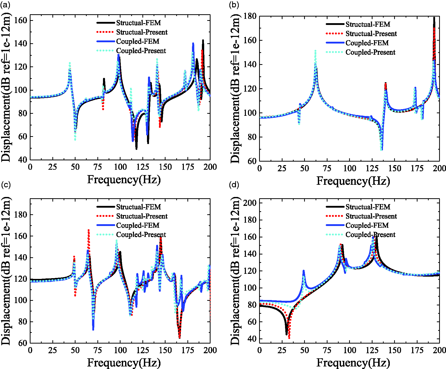
Responses of the L-shaped plate and the L-shaped plate–cavity coupling system filled with air under the excitation of point forces (F₁ and F₂). (a) Displacement at (0.8,0.1) in plate 1. (b) Displacement at (0.5,0.6) in plate 2. (c) Displacement at (0.8,0.1) in plate 1. (d) Displacement at (0.5,0.6) in plate 2.

It is shown which response of coupling model with various BC and various materials under point source excitation in Figure 6. The coupling system dimensions and materials used in Figure 6 are identical to those of Figure 4. The unit point sound source position in Figure 6 is located at the center point (0.7, 0.6, and 0.5) of the cavity. It can be known that the response consequents calculated by the Fourier series method are correct by comparing with the response consequents obtained by the FEM.

Figure 6.

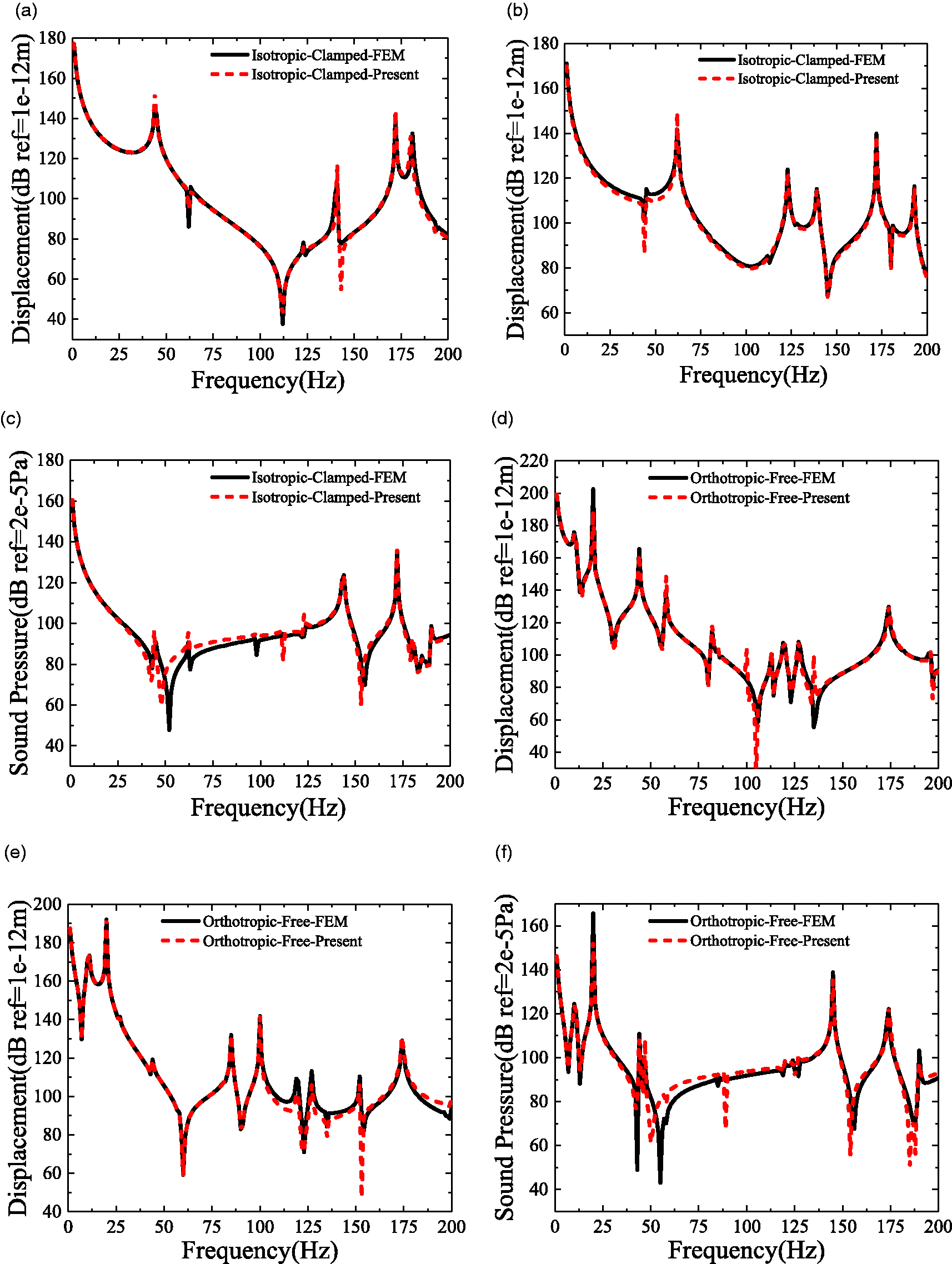
Responses of the L-shaped plate–cavity coupling system under the excitation of a point sound source under different boundary condition and material. (a) Displacement at (0.7,0.6) in plate 1. (b) Displacement at (0.5,0.6) in plate 2. (c) Sound Pressure at (0.75,0.15,0.2). (d) Displacement at (0.7,0.6) in plate 1. (e) Displacement at (0.5,0.6) in plate 2. (f) Sound Pressure at (0.75,0.15,0.2).

Then, we explore the impact of impedance on the forced response. Figure 7 shows the response curve of the coupling model under the effect of forces and sound source. Here, the model parameters and the locations of the forces and sound source are identical to those in Figures 4 and 6. Plates’ material is selected as the Material I. The impedance values of the four non-related surfaces are set as rigid and Z = ρ_airc_air(100-j), respectively. It can speculate from Figures, which the existence of impedance affect the vertex value of the response curve, however, the tendency of the displacement and sound pressure curve does not change.

Figure 7.

Responses of the L-shaped plate–cavity coupling system with impendence value under the excitation of point forces (F₁ and F₂) (a) to (c) and a point sound source (d) to (f). (a) Displacement at (0.8,0.1) in plate 1. (b) Displacement at (0.65,0.15) in plate 2. (c) Sound Pressure at (0.75,0.15,0.2). (d) Displacement at (0.8,0.1) in plate 1. (e) Displacement at (0.5,0.6) in plate 2. (f) Sound Pressure at (0.75,0.15,0.2).

Finally, effects of the L-shaped plate’ materials on the forced response are investigated. The results of the L-shaped plate–cavity system filled with air under different materials of two plates and the excitation of point forces are studied. The dimensions and BC of Figure 8 are the same as those shown in Table 4. Since the two plates of the L-shaped plate have the same sizes, and the action points are at the midpoint of the plate, the two positions on the plate 1 including the force point and the non-force point and the center point of the cavity are selected as response analysis. It can be seen from the figure that when the two plates are selected as isotropic materials, the trend of displacement response curves of the L-shaped plates are consistent, and the displacement response of any plate on the L-shaped plates has a relationship with the material of the plate. The trend of sound pressure curve is consistent, and sound pressure curve is located inside the two curves, which are the sound pressure response curves, when the two plates are selected from the same materials. When the two plates are made of orthotropic materials, the displacement curve in the 0–50 Hz is related to the two plates. When the frequency is greater than 50 Hz, the displacement response is related to the material of the plate where the test point is located. The trend of displacement response is consistent with the displacement response under the same materials, but the displacement slightly reduced and offset at the peak. The sound pressure of the cuboid cavity is related to the materials of L-shaped plates. Figure 9 displays the response of the L-shaped plate–cavity coupling model existed air under different materials of two plates and the action of the point source. The dimensions and boundary situations of Figure 9 are the same as in Figure 8. The position of the point source is displaced from the center of the cuboid cavity. The same conclusions, as in Figure 7, can be obtained by response analysis.

Figure 8.

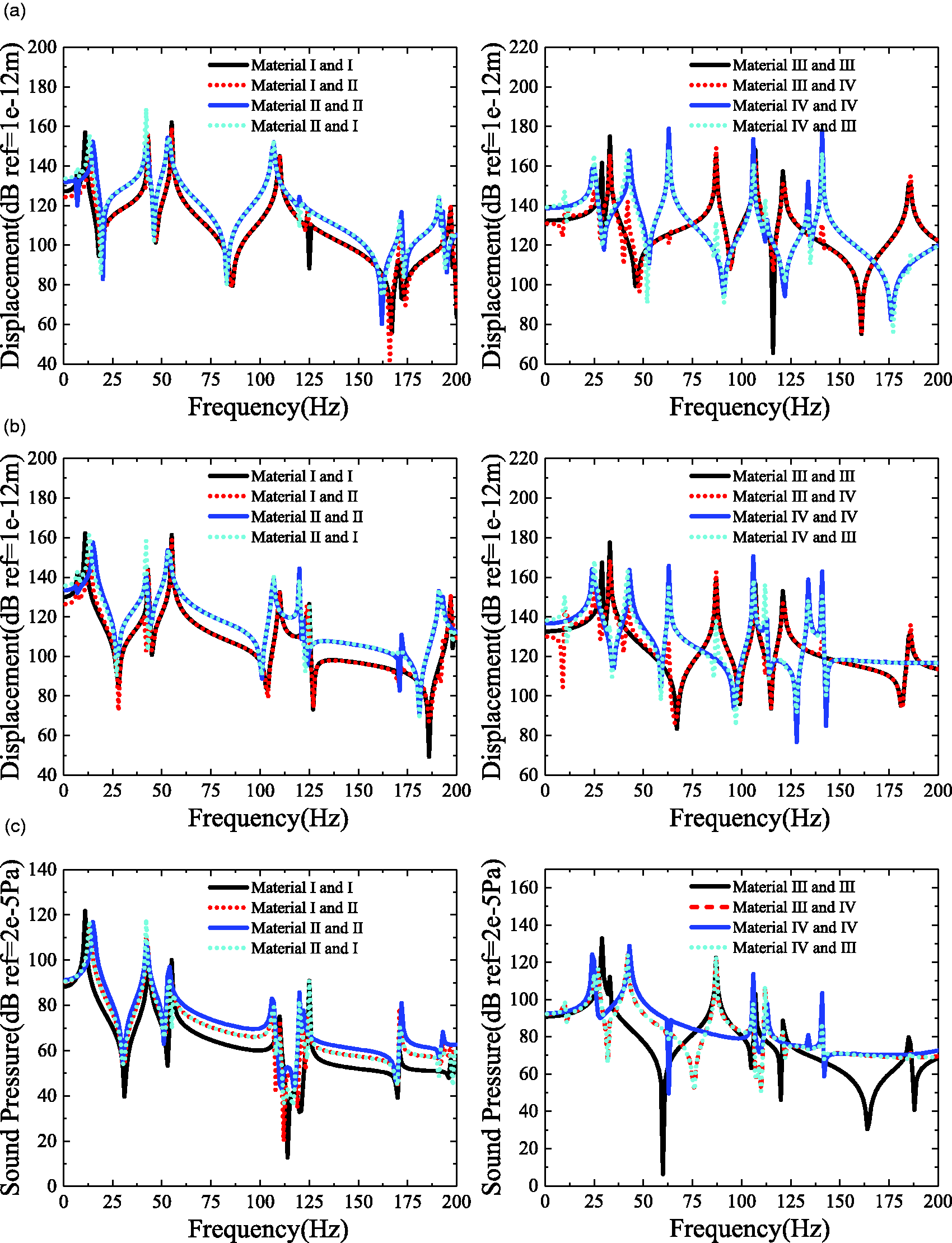
Responses of the L-shaped plate–cavity coupling system filled with air under different materials of two plates and the excitation of point forces (F₁ and F₂). (a) Displacement at (0.5,0.5) in plate1. (b) Displacement at (0.7,0.6) in plate1. (c) Sound Pressure at (0.5,0.5,0.5).

Figure 9.

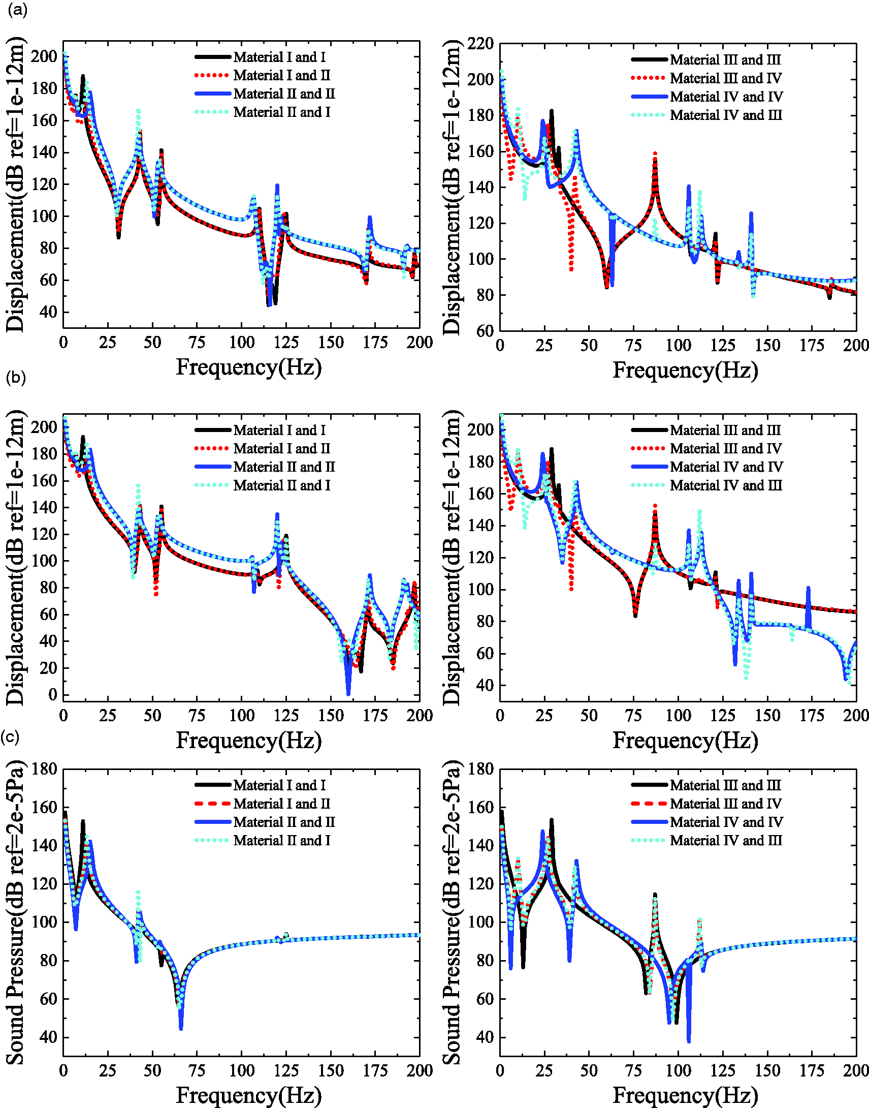
Responses of the L-shaped plate–cavity coupling system filled with air under different materials of two plates and the excitation of a point sound source. (a) Displacement at (0.5,0.5) in plate1. (b) Displacement at (0.7,0.6) in plate1. (c) Sound Pressure at (0.5,0.5,0.5).

Conclusions

In this paper, it is studied by Fourier series method that the vibro-acoustic behaviors of coupling model including the L-shaped plate and a cuboid cavity. The natural frequency of the L-shaped plate–cavity coupling system is analyzed in this paper. In this paper, the displacements admissible functions of the L-shaped plate are generally set as the sum of two cosines’ product and two polynomials. Sound pressure admissible functions of the cuboid acoustic cavity can be written as the sum of three cosines’ product and six polynomials. By contrasting with the results of FEM, the good convergence and consistency of the method are demonstrated. The vibro-acoustic research of the L-shaped plate–cavity coupling system under a point force or a point source is studied particularly in this paper. This method in this paper is further extended to the analysis of other plate structure problems, such as U-shaped plate–cavity system.

Here are some guiding conclusions:

The natural frequency will increase as the increase of the spring stiffness value. At the same time, the response curves will change with it. The cuboid acoustic cavity has impedance wall that effectively attenuates the resonance. This is important to reduce vibration and control noise.

By selecting orthotropic degrees and plate thicknesses, it can be controlled that the natural frequencies of the coupling system. For example, increasing the orthotropic degree will raise the natural frequency.

When the materials of two plates are selected from different materials of the same type, the displacement response is related to the material of the plate where the test point is located. But the sound pressure result is related to materials of the two plates of the L-shaped plate.