An adaptive sampling procedure for parametric model order reduction by matrix interpolation

Abstract

An adaptive sampling approach for parametric model order reduction by matrix interpolation is developed. This approach is based on an efficient exploration of the candidate parameter sets and identification of the points with maximum errors. An error indicator is defined and used for fast evaluation of the parameter points in the configuration space. Furthermore, the exact error of the model with maximum error indicator is calculated to determine whether the adaptive sampling procedure reaches a desired error tolerance. To improve the accuracy, the orthogonal eigenvectors are utilized as the reduced-order basis. The proposed adaptive sampling procedure is then illustrated by application in the moving coil of electrical-dynamic shaker. It is shown that the new method can sample the parameter space adaptively and efficiently with the assurance of the resulting reduced-order models’ accuracy.

Introduction

Finite element method (FEM) has become a common approach to simulate the behavior of complex physical systems. However, large-scale complex systems usually result in high-dimensional computational models, leading to prohibitively intensive computations. To overcome this problem, model order reduction (MOR) methods have been employed to obtain a low-dimensional but accurate approximation of the large-scale dynamic system by projecting the high-dimensional model (HDM) onto a low-dimensional subspace described by an ROB. The commonly used MOR methods include proper orthogonal decomposition, Krylov-subspace based methods, and truncated balanced realization. ¹ And these techniques have already applied in some areas like optimization and control,^2,3 uncertainty quantification, ⁴ and parameter identification. ⁵

However, structural models are usually parameter-dependent. It is inefficient and impractical to reduce the model order repeatedly at different parameter values. This has promoted the study of parametric model order reduction (PMOR) technique, which aims to generate a parametric ROM approximating the original full-order dynamical system with high fidelity over the range of parameters. As for the PMOR strategies, Benner et al. ⁶ conducted an overall survey on the existing PMOR methods, including the global and local approaches. Geuss et al. ⁷ researched various matrix interpolatory methods and proposed a general method to unite them.

It is the fundamental issue how the parameter dependence is imported. For the systems explicitly dependent on parameters, ⁸ the standard MOR strategies have been extended and applied, like multi-dimensional moment matching algorithms. ⁹ While for the systems with affine parametric dependency, the global basis and interpolation among local bases approaches ¹⁰ are both effective in reducing the system order.

As for the implicit and non-affine parametric dependency, the matrix interpolatory PMOR framework is the most appropriate and general approach. Panzer et al. ¹¹ interpolated the low-dimensional local system matrices via weighting functions to achieve the parametric ROMs. Amsallem et al. ¹² interpolated the order-reduced matrices on a tangent space to eliminate the nonlinearity of precomputed ROMs.

The most fundamental and critical step in the existing PMOR methods is the sampling strategy of parameter space. The distribution of the parameter sample points should enable the surrogate model to capture the underlying parametric dependence to a maximum extent. There have been two major approaches aimed at finding the optimal sampling points with largest error indicator in the parameter space. The first one simply calculates the posteriori error indicator of a large discrete sets of candidate parameter values and finds the optimal point with max errors.^13–15 It is very simple to compute but may suffer from the curse of dimensionality for multi-dimensional parameter space. The other one solves the model-constrained optimization problem using gradient-based approaches and selects the solution as the sampling point. ¹⁶ This kind of approach may not find the global optimal solution, but only the local ones. Besides, this approach can only be exploited in models with affine parametric dependency because of the need to express full-order system matrices explicitly.

Most of the existing adaptive sampling approaches are based on reduced basis PMOR methods. Few literatures applied the adaptive sampling strategy to matrix interpolatory PMOR framework. Varona and Lohmann ¹⁷ utilized the distance between subspaces as a measure and proposed an adaptive sampling procedure combined with PMOR by matrix interpolation. This approach can sample the parameter space adaptively and automatically, but it cannot evaluate the precision of the algorithm due to the absence of error estimation.

This article proposes an automatic adaptive parameter space sampling procedure for matrix interpolatory PMOR framework. It is applicable to the general case, in which the arbitrary parameter dependence is considered. To sample the parameter space adaptively, an error indicator for rapid error evaluation is introduced. The location of an optimal sample point is thereby identified by a direct exhaustive exploration of a large discrete candidate parameter sets. The maximum of the residual between the HDM and the ROM at this parameter value is subsequently calculated to monitor the convergence rate and used as the termination criteria. In addition, the orthogonal eigenvectors are applied as the ROB to improve the accuracy. This method combines the benefits of matrix interpolatory PMOR and those of adaptive sampling procedure. And it can serve as a substitute for the classical offline ROMs generation algorithm in PMOR.

It is organized as follows: The next section describes the classical matrix interpolatory PMOR method in detail. “The proposed adaptive sampling procedure” section outlines the automatic adaptive PMOR framework and summarizes the algorithm of generating the offline ROMs database. In “Numerical example” section, the proposed strategy is exploited to adaptively generate the parametric ROM for the moving coil of electrical-dynamic shaker. Results of the ROM and HDM are compared to illustrate the advantage and validity of the proposed approach.

The classical matrix interpolatory PMOR framework

Based on the classical MOR method, the matrix interpolatory PMOR approach has become an essential technique for reducing the order of large FE models with varying parameter configurations. For parameter-dependent linear system, the structural–dynamical equation can be described as

$$\mathit{M}\left(\mathit{p}\right)\cdot \ddot{\mathit{x}}+\mathit{D}\left(\mathit{p}\right)\cdot \dot{\mathit{x}}+\mathit{K}\left(\mathit{p}\right)\cdot \mathit{x}=\mathit{F}\left(\mathit{p}\right)$$

(1)

where $\mathit{M}\left(\mathit{p}\right),\mathit{D}\left(\mathit{p}\right),\mathit{K}\left(\mathit{p}\right)\in {ℝ}^{n\times n}$ are the parameter-dependent mass, damping, stiffness, and force matrices, respectively. $\mathit{x},\mathit{F}\left(\mathit{p}\right)\in {ℝ}^{n\times 1}$ is the displacement vector force vectors, and n is the number of degree of freedom (DOF) of the system.

The uniform or random sampling method can be applied to sample the continuous parameter field p and generate a rich set of data with full coverage of the parameter space.

Assume now that the uniform sampling method is utilized to obtain a discrete set of parameter samples p _i for i = 1… m. The large-scale FE model is then generated at each corresponding discrete parameter value

$${\mathit{M}}_i\cdot {\ddot{\mathit{x}}}_i+{\mathit{D}}_i\cdot {\dot{\mathit{x}}}_i+{\mathit{K}}_i\cdot {\mathit{x}}_i={\mathit{F}}_i.$$

(2)

Then, each local large-scale model is reduced individually by the use of MOR methods. The general practice of this approach is to construct a low-dimensional subspace ${\mathit{V}}_i\in {ℝ}^{n\times r}$ and approximate the original displacement vector ${\mathit{x}}_i\in {ℝ}^n$ with an order-reduced vector ${\mathit{x}}_{\mathit{ri}}\in {ℝ}^r$ (in general case, $r\ll n$ )

$${\mathit{x}}_i\approx {\mathit{V}}_i\cdot {\mathit{x}}_{\mathit{ri}}$$

(3)

Substituting equation (3) into equation (2) and multiplying the equation from the left by the transpose of the matrix V _i results in the order-reduced structural dynamic models at the discrete parameter values p _i , as

$${\mathit{M}}_{\mathit{ri}}\cdot {\ddot{\mathit{x}}}_{\mathit{ri}}+{\mathit{D}}_{\mathit{ri}}\cdot {\dot{\mathit{x}}}_{\mathit{ri}}+{\mathit{K}}_{\mathit{ri}}\cdot {\mathit{x}}_{\mathit{ri}}={\mathit{F}}_{\mathit{ri}}$$

(4)

where ${\mathit{M}}_{r,i}\text{=}{\mathit{V}}_i^{\text{T}}{\mathit{M}}_i{\mathit{V}}_i,{\mathit{D}}_{r,i}={\mathit{V}}_i^{\text{T}}{\mathit{D}}_i{\mathit{V}}_i,{\mathit{K}}_{r,i}={\mathit{V}}_i^{\text{T}}{\mathit{K}}_i{\mathit{V}}_i\in {ℝ}^{r\times r}$ are all reduced system matrices, and ${\mathit{F}}_{\mathit{ri}}={\mathit{V}}_i^{\text{T}}{\mathit{F}}_i\in {ℝ}^{r\times 1}$ is the reduced force vector. Each local reduced model has a unique basis vector ${\mathit{V}}_i\in {ℝ}^{n\times r}$ .

According to Antoulas, ¹ Krylov-subspace reduction methods extract low-dimensional projection basis and project the HDM onto the subspace. The resulting ROM maintains the dynamic characteristics of original systems and has many advantages like high calculating stability, precision, and efficiency. Hence this kind of method is widely utilized in the classical PMOR framework.

With respect to the second-order dynamic systems, Bai ¹⁸ proposed a modified version of the Arnoldi process to construct internally orthogonalized basis vectors spanning the Krylov subspace. The modified Arnoldi process is utilized in this paper. One can refer to Bai¹⁸ for the detailed algorithm.

The subspace induced by matrices K_i, M_i, and vector F_i is defined as

$${\mathit{V}}_i=\mathit{span}\left(K_r\left\{{\mathit{K}}_i^{-1}{\mathit{M}}_i,{\mathit{K}}_i^{-1}{\mathit{F}}_i\right\}\right)=\mathit{span}\left({\mathit{b}}_i,{\mathit{A}}_i{\mathit{b}}_i,{\mathit{A}}_i^2{\mathit{b}}_i,\cdots \right)$$

(5)

where ${\mathit{b}}_i={\mathit{K}}_i^{-1}{\mathit{F}}_i$ and ${\mathit{A}}_i={\mathit{K}}_i^{-1}{\mathit{M}}_i$ .

According to equation (4), we can obtain m ROMs. However, since these reduced-order system matrices are defined in different coordinate systems, the direct interpolation of these matrices may be meaningless. Therefore, congruence transformations should be performed to adjust the local system matrices and basis vectors. As mentioned above, Panzer et al. ¹¹ built a total matrix of all the basis vectors and conducted singular value decomposition (SVD) of this matrix to achieve the rth-order most important directions as the reference basis vector. All the precomputed local ROMs are then transformed into a consistent set of generalized coordinates.

Although the results are relatively accurate, the SVD procedure has to be repeated when a new parameter sample added, which could be time-consuming for multi-dimensional parametric large models. Therefore, an improved method presented by Amsallem and Farhat [19] is exploited in this research to adjust the local reduced models.

First of all, the following minimization problems is considered

$$\underset{\mathit{R}\in \text{O}\left(r\right)}{\min }{\Vert {\mathit{V}}_i\mathit{R}-{\mathit{V}}_0\Vert }_F^2$$

(6)

where $\text{O}\left(r\right)$ represents a set of orthogonal square matrices in ${ℝ}^{r\times r}$ , the subscript F denotes the Frobenius norm, and any precomputed basis can be set as the standard vector ${\mathit{V}}_0$ .

From equation (6), the following maximization problem can be derived as

$$\underset{\mathit{R}\in \text{O}\left(r\right)}{\max }\text{tr}\left({\mathit{R}}^{\text{T}}{\mathit{V}}_i^{\text{T}}{\mathit{V}}_0\right)$$

(7)

where the symbol $\text{tr}$ denotes the trace of matrices.

In equation (7), multiplication of the basis vectors is defined as follows

$${\mathit{P}}_{i,0}={\mathit{V}}_i^{\text{T}}{\mathit{V}}_0$$

(8)

Then, we can simplify equation (7) as

$$\underset{\mathit{R}\in \text{O}\left(r\right)}{\max }\text{tr}\left({\mathit{R}}^{\text{T}}{\mathit{P}}_{i,0}\right)$$

(9)

According to Amsallem and Farhat, ¹⁹ the analytical solution to equation (9) is

$${\mathit{R}}_{i,0}^{*}={\mathit{U}}_{i,0}{\mathit{Z}}_{i,0}^{\text{T}}$$

(10)

where ${\mathit{U}}_{i,0}$ and ${\mathit{Z}}_{i,0}^{\hspace{0.17em}}$ are computed by the SVD of ${\mathit{P}}_{i,0}$ as follows

$${\mathit{P}}_{i,0}={\mathit{U}}_{i,0}{\mathbf{\Sigma }}_{i,0}{\mathit{Z}}_{i,0}^{\text{T}}$$

(11)

The relation between different coordinate systems can thereby be expressed as

$${\mathit{x}}_i={\mathit{V}}_i{\mathit{x}}_{\mathit{ri}}={\mathit{V}}_i^{*}{\mathit{x}}_{\mathit{ri}}^{*}$$

(12)

where ${\mathit{V}}_i^{*}={\mathit{V}}_i{\mathit{R}}_{i,0}^{*}.$

Inserting the coordinate transformation relation equation (12) in equation. (2), multiplying from the left by ${\mathit{V}}_i^{*}$ and comparing the precomputed models in equation (4) leading to the ROMs expressed in the same generalized coordinate system

$${\mathit{M}}_{\mathit{ri}}^{\text{*}}\cdot {\ddot{\mathit{x}}}_{\mathit{ri}}^{\text{*}}+{\mathit{D}}_{\mathit{ri}}^{\text{*}}\cdot {\dot{\mathit{x}}}_{\mathit{ri}}^{\text{*}}+{\mathit{K}}_{\mathit{ri}}^{\text{*}}\cdot {\mathit{x}}_{\mathit{ri}}^{\text{*}}={\mathit{F}}_{\mathit{ri}}^{\text{*}}$$

(13)

where ${\mathit{M}}_{\mathit{ri}}^{\text{*}}={\mathit{R}}_{i,0}^{*}{\hspace{0.17em}}^{\text{T}}{\mathit{M}}_{\mathit{ri}}^{\hspace{0.17em}}{\mathit{R}}_{i,0}^{*},{\mathit{D}}_{\mathit{ri}}^{\text{*}}={\mathit{R}}_{i,0}^{*}{\hspace{0.17em}}^{\text{T}}{\mathit{D}}_{\mathit{ri}}^{\hspace{0.17em}}{\mathit{R}}_{i,0}^{*},{\mathit{K}}_{\mathit{ri}}^{\text{*}}={\mathit{R}}_{i,0}^{*}{\hspace{0.17em}}^{\text{T}}{\mathit{K}}_{\mathit{ri}}^{\hspace{0.17em}}{\mathit{R}}_{i,0}^{*},{\mathit{F}}_{\mathit{ri}}^{\text{*}}={\mathit{R}}_{i,0}^{*}{\hspace{0.17em}}^{\text{T}}{\mathit{F}}_{\mathit{ri}}^{\hspace{0.17em}}.$

After the compatible reduced-order matrices obtained, the new matrices at the given parameter value can be constructed by direct interpolation or interpolation on the tangent matrix manifold. In comparison, interpolation on tangent manifold can weaken the influence of nonlinearity, and the result is more accurate. Thus, it is applied in this paper to construct the parametric model.

First of all, a reference matrix is selected, and the interpolation will be performed in the space tangent to the manifold at that reference. For example, we set ${\mathit{K}}_{r,1}^{*}$ as the reference matrix and suppose ${\Upsilon }_{{\mathit{K}}_{r,1}^{*}}$ to be the corresponding tangent space. Then, all the other local reduced-order matrices ${\mathit{K}}_{\mathit{ri}}^{*}$ can be projected onto the tangent space ${\Upsilon }_{{\mathit{K}}_{r,1}^{*}}$ by the logarithmic map

$${\mathbf{\Theta }}_i^{\mathit{K}}={\text{Log}}_{{\mathit{K}}_{r,1}^{*}}\left({\mathit{K}}_{\mathit{ri}}^{*}\right)\text{=log}\left[{\mathit{K}}_{\mathit{ri}}^{*}{\left({\mathit{K}}_{r,1}^{*}\right)}^{-1}\right]\in {\Upsilon }_{{\mathit{K}}_{r,1}^{*}}$$

(14)

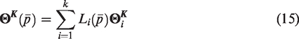
After all the reduced-order matrices projected, we can obtain the reduced-order model matrices at a new parameter point by matrix interpolation. As for the interpolation method, Lagrange interpolation could provide both enough accuracy and efficiency. Therefore, it is used in the online stage

$${\mathbf{\Theta }}_{\hspace{0.17em}}^{\mathit{K}}\left(\overline{p}\right)={\displaystyle \sum _{i=1}^k{L}_i\left(\overline{p}\right){\mathbf{\Theta }}_i^{\mathit{K}}}$$

(15)

where $L_i\left(\overline{p}\right)$ are the Lagrange basis functions. Then, we project $\Theta \left(\overline{p}\right)$ back to the original space by the exponential map

$${\mathit{K}}_r^{*}\left(\overline{p}\right)={\text{Exp}}_{{\mathit{K}}_{r,1}^{*}}\left[{\mathbf{\Theta }}^{\mathit{K}}\left(\overline{p}\right)\right]=\exp \left[{\mathbf{\Theta }}^{\mathit{K}}\left(\overline{p}\right)\right]{\mathit{K}}_{r,1}^{*}$$

(16)

Then, ${\mathit{D}}_r^{*}\left(\overline{p}\right),{\mathit{M}}_r^{*}\left(\overline{p}\right)$ can also be obtained by setting ${\mathit{D}}_{r,1}^{*},{\mathit{M}}_{r,1}^{*}$ as the reference matrix, respectively. As the reduced-order matrices are small in dimension, the logarithmic and exponential algorithms in equations (14) and (16) just cost little time and can be solved more easily.

In this way, we can obtain the reduced matrices and basis vectors and then calculate the order-reduced response ${\mathit{x}}_r^{*}\left(\overline{p}\right)$ and eigenvector ${\mathbf{\Phi }}_r^{*}\left(\overline{p}\right)$ by the use of ${\mathit{K}}_r^{*}\left(\overline{p}\right),{\mathit{M}}_r^{*}\left(\overline{p}\right),{\mathit{D}}_r^{*}\left(\overline{p}\right),{\mathit{F}}_r^{*}\left(\overline{p}\right)$ at this specific parameter value. They are then projected back to the original space to get the results expressed in real physical coordinate by the formula

$$\mathit{x}\left(\overline{p}\right)={\mathit{V}}^{*}\left(\overline{p}\right)\cdot {\mathit{x}}_r^{*}\left(\overline{p}\right)$$

(17)

$$\mathbf{\Phi }\left(\overline{p}\right)={\mathit{V}}^{*}\left(\overline{p}\right)\cdot {\mathbf{\Phi }}_r^{*}\left(\overline{p}\right)$$

(18)

The complete calculation procedure of PMOR method can be decomposed into offline and online steps. The calculation in the online stage includes only equations (14) to (16). But the focus of PMOR method is on the offline ROMs building steps. Thus, we summarize the offline ROMs generation algorithm of classical PMOR as follows:

Algorithm 1. Classical offline ROMs generation algorithm.

Input: Parameter domain $\Omega$ , sampling points numbers $N$

Output: Compatible ROMs ( ${\mathbf{\Theta }}_i^{\mathit{K}},{\mathbf{\Theta }}_i^{\mathit{M}},{\mathbf{\Theta }}_i^{\mathit{D}},{\mathit{F}}_{\mathit{ri}}^{\text{*}},{\mathit{V}}_i^{*}$ )

Uniformly select a set of $N$ candidate parameters

for i =1,…, N do

 Generate the corresponding matrices ${\mathit{K}}_i,{\mathit{M}}_i,{\mathit{D}}_i,{\mathit{F}}_i$

 Calculate ROBs ${\mathit{V}}_i^{\hspace{0.17em}}$ by use of the modified Arnoldi process.

 Construct the ROMs ( ${\mathit{K}}_{\mathit{ri}},{\mathit{M}}_{\mathit{ri}},{\mathit{D}}_{\mathit{ri}},{\mathit{F}}_{\mathit{ri}},{\mathit{V}}_i$ )

end for

Choose a ROB ${\mathit{V}}_1^{\hspace{0.17em}}$ as the reference basis.

for i =1,…, N do

 Calculate the transformation matrix ${\mathit{R}}_{i,0}^{*}$ at $p_i$

 Adjust the local ROMs and obtain ${\mathit{K}}_{\mathit{ri}}^{\text{*}},{\mathit{M}}_{\mathit{ri}}^{\text{*}},{\mathit{D}}_{\mathit{ri}}^{\text{*}},{\mathit{F}}_{\mathit{ri}}^{\text{*}},{\mathit{V}}_i^{*}$ at $p_i$

end for

Choose matrices ${\mathit{K}}_{r1}^{\text{*}},{\mathit{M}}_{r1}^{\text{*}},{\mathit{D}}_{r1}^{\text{*}}$ as the reference matrices respectively.

for i =1,…, N do

 Project the matrices onto the tangent space and obtain ${\mathbf{\Theta }}_i^{\mathit{K}},{\mathbf{\Theta }}_i^{\mathit{M}},{\mathbf{\Theta }}_i^{\mathit{D}}$ at $p_i$

end for

Conclusively, the entire calculation flow of classical PMOR method can be summarized as: generate the uniformly distributed compatible ROMs in the offline stage, calculate the new ROM and the reduced-order results for the given parameter value in the online stage, and project them back to the original physical coordinate.

The proposed adaptive sampling procedure

Although the classical PMOR method can achieve satisfactory accuracy, it cannot provide the error estimation, convergence rate, and termination criteria. Thus, the minimum number of sample points to satisfy the predefined error cannot be determined. Besides, with respect to the uniform sampling approach, one has to regenerate all the precomputed ROMs when adding a new sample point. Another drawback is that the orthonormal basis of the Krylov subspace achieved by Arnoldi process can match only limited moments. To guarantee the accuracy, the order of the ROB has to be high enough, which is relatively time-consuming. Therefore, we propose an adaptive PMOR procedure to sample the parameter space and generate the ROMs efficiently and accurately.

First, the ROB V in equation (5) can be set as the eigenvectors for the structural dynamic system. For the structural dynamic models in equation (2), the eigenvalues ${\mathit{\lambda }}_i$ and eigenvectors ${\mathbf{\Phi }}_i$ can be obtained by

$$\left({\mathit{K}}_i-{\mathit{\lambda }}_i{\mathit{M}}_i\right){\mathbf{\Phi }}_i=0$$

(19)

By selecting r modes vectors as the ascending order of the magnitude of the eigenvalues, we can obtain the first r columns eigenvectors ${\mathbf{\Phi }}_{i,r}$ and use them as ROBs. These eigenvectors should satisfy the following orthogonality condition

$${\mathit{V}}^{\text{T}}\mathit{V}=\mathit{I}\in {ℝ}^{r\times r}$$

(20)

Assume the orthogonal eigenvectors after a Gram–Schmidt procedure as ${\mathbf{\Phi }}_{i,r}^{\text{S}}$ , hence

$${\left({\mathbf{\Phi }}_{i,r}^{\text{S}}\right)}^{\text{T}}{\mathbf{\Phi }}_{i,r}^{\text{S}}=\mathit{I}\in {ℝ}^{r\times r}$$

(21)

Then, the order-reduced response and eigenvector defined in equations (17) and (18) can be replaced by the formula

$$\mathit{x}\left(\overline{p}\right)={\mathbf{\Phi }}^{\text{S}}\left(\overline{p}\right)\cdot {\mathit{x}}_r\left(\overline{p}\right)$$

(22)

$$\mathbf{\Phi }\left(\overline{p}\right)={\mathbf{\Phi }}^{\text{S}}\left(\overline{p}\right)\cdot {\mathbf{\Phi }}_r\left(\overline{p}\right)$$

(23)

The goal of the adaptive parameter sampling approach is to estimate, at each iteration N_iter, the parameter $u^{\max }$ maximizing the error indicator over the set ℂ. These full-order models with maximum error indicators are subsequently generated to evaluate the exact relative errors.

This approach proceeds in two phases. In the first phase, a candidate parameter set is chosen as

$$ℂ=\left\{u^1,\cdots ,u^{N_c}\right\}\subset \Omega$$

(24)

Then, we compute the error estimator over the set ℂ. To define the error indicator for fast estimation, we substitute the eigenvector $\mathbf{\Phi }\left(u^i\right)$ into the characteristic equation (19) and obtain the residual vector as

$$r\text{=}\left(\mathit{K}\left(u^i\right)-\mathit{\lambda }\mathit{M}\left(u^i\right)\right)\mathbf{\Phi }\left(u^i\right)$$

(25)

where $\mathbf{\Phi }\left(u^i\right)$ is calculated by equation (23), $\mathit{\lambda }$ and ${\mathbf{\Phi }}_r\left(u^i\right)$ in equation (23) is calculated by the use of the reduced order matrices ${\mathit{K}}_r^{*}\left(u^i\right)$ and ${\mathit{M}}_r^{*}\left(u^i\right)$ , these matrices together with the full order matrices $\mathit{K}\left(u^i\right),\mathit{M}\left(u^i\right)$ are all calculated through direct Lagrange interpolation. Thus, the cost of evaluating error indicator at multiple discrete parameter values could be relatively cheap.

To eliminate the accumulated error, we multiply the residual vector from the left by $\mathbf{\Phi }{\left(u^i\right)}^{\text{T}}$ and obtain the following error indicator

$${\epsilon }_{\text{1}}\text{=max}\left(\mathbf{\Phi }{\left(u^i\right)}^{\text{T}}\left(\mathit{K}\left(u^i\right)-\mathit{\lambda }\mathit{M}\left(u^i\right)\right)\mathbf{\Phi }\left(u^i\right)\right)$$

(26)

After this error indicator calculated for the parameter values $u^i,i=1,2\cdots ,N_c$ , we thereby build the following error pool to construct a surrogate model for the error ${\epsilon }_1^{\hspace{0.17em}}$ as a function of the parameter values

$$E=\left\{\left(u_{\hspace{0.17em}}^1,{\epsilon }_1^1\right),\left(u^2,{\epsilon }_1^2\right),\cdots ,\left(u^{N_c},{\epsilon }_1^{N_c}\right)\right\}$$

(27)

At each iteration N_iter of the adaptive sampling process, the parameter value $u^{\max }$ is chosen as the maximizer

$$u^{\max }=\underset{u\in \Omega }{\arg \mathrm{\hspace{0.17em}max}}E\left(u\right)$$

(28)

The parameter values are then used in the next phase to generate corresponding full-order matrices. After these matrices are reduced, the overall exact errors between the HDM and the ROM are evaluated and applied to monitor the convergence of the algorithm and terminate the procedure automatically. The exact errors of frequencies and modal shapes are defined as

$${\epsilon }_2\text{=}\frac{\left|\sqrt{{\mathit{\lambda }}_{u^{\max }}}-\sqrt{\mathit{\lambda }\left(u^{\max }\right)}\right|}{\sqrt{{\mathit{\lambda }}_{u^{\max }}}}$$

(29)

$${\epsilon }_3\text{=}\frac{\max \left|\left|{\mathbf{\Phi }}_{u^{\max }}^{\text{N}}\right|-\left|{\mathbf{\Phi }}^{\text{N}}\left(u^{\max }\right)\right|\right|}{\max \left|{\mathbf{\Phi }}_{u^{\max }}^{\text{N}}\right|}$$

(30)

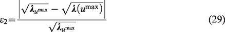
It should be noted that the subscripts $u^{\max }$ and $u^{\max }$ in brackets represent the results calculated using the exact model and the PMOR method at parameter value $u^{\max }$ , respectively. The time-consuming calculation of the exact error is only performed at the parameter value where the error indicator is max. The regularized modal shape vectors ${\mathbf{\Phi }}_{u^{\max }}^{\text{N}}$ and ${\mathbf{\Phi }}^{\text{N}}\left(u^{\max }\right)$ satisfy the following orthogonality condition

$${\left({\mathbf{\Phi }}_{u^{\max }}^{\text{N}}\right)}^{\text{T}}{\mathit{M}}_{u^{\max }}{\mathbf{\Phi }}_{u^{\max }}^{\text{N}}=\mathit{I}$$

(31)

$${\left({\mathbf{\Phi }}^{\text{N}}\left(u^{\max }\right)\right)}^{\text{T}}\mathit{M}\left(u^{\max }\right){\mathbf{\Phi }}^{\text{N}}\left(u^{\max }\right)=\mathit{I}$$

(32)

where ${\mathit{M}}_{u^{\max }}$ and $\mathit{M}\left(u^{\max }\right)$ are the exact and interpolated mass matrices at parameter $u^{\max }$ .

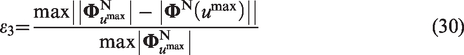
In order to obtain the regularization form of the modal shape vectors, we should regularize them columnwise. For the kth column of ${\mathbf{\Phi }}_{u^{\max }}^{\hspace{0.17em}}$ , the regularization equation can be described as

$${\mathbf{\Phi }}_{u^{\max },k}^{\text{N}}=\frac{{\mathbf{\Phi }}_{u^{\max },k}^{\hspace{0.17em}}}{\sqrt{{\mathbf{\Phi }}_{u^{\max },k}^{\text{T}}{\mathit{M}}_{u^{\max }}{\mathbf{\Phi }}_{u^{\max },k}^{\hspace{0.17em}}}}$$

(33)

And ${\mathbf{\Phi }}_{u^{\max }}^{\text{N}}$ can be obtained after all the columns regularized. As equation (25), the exact error of response is defined as the maximum of the low-dimensional residual

$$\begin{array}{l}{\epsilon }_4\text{=max}|\mathbf{\Phi }{\left(u^{\max }\right)}^{\text{T}}{\mathit{M}}_{u^{\max }}\mathbf{\Phi }\left(u^{\max }\right)\cdot \ddot{\mathit{x}}\left(u^{\max }\right)+\mathbf{\Phi }{\left(u^{\max }\right)}^{\text{T}}{\mathit{D}}_{u^{\max }}\mathbf{\Phi }\left(u^{\max }\right)\cdot \dot{\mathit{x}}\left(u^{\max }\right)\\ +\mathbf{\Phi }{\left(u^{\max }\right)}^{\text{T}}{\mathit{K}}_{u^{\max }}\mathbf{\Phi }\left(u^{\max }\right)\cdot \mathit{x}\left(u^{\max }\right)-\mathbf{\Phi }{\left(u^{\max }\right)}^{\text{T}}{\mathit{F}}_{u^{\max }}|\end{array}$$

(34)

where ${\mathit{K}}_{u^{\max }},{\mathit{M}}_{u^{\max }},{\mathit{D}}_{u^{\max }},{\mathit{F}}_{u^{\max }}$ are the exact stiffness, mass, damping, and force matrices generated at the specific parameter $u^{\max }$ .

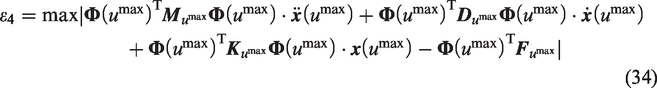
After exploring the parameter space and identifying the sampling points with maximum error indicators, we subsequently insert new parameter samples at these locations. In this paper, the regular parameter grid is used. The corresponding parameter points of a regular grid with dimension d have a certain structure which must be preserved during the inserting procedure. For one-dimensional parameter space as shown in Figure 1(a), we directly place a new sample in the space and utilize the interpolation method as equation (15). While for multi-dimensional case, it is a little more complicated. In addition to the point with maximum errors, we have to insert more points to preserve the structure of regular grids. Consider a two-dimensional grid as shown in Figure 1(b), the new inserted points are denoted by red circles, and the point with the maximum error indicator is indicated with a blue cross.

Figure 1.

Points insertion for regular grids: (a) one-dimensional grid and (b) two-dimensional grid.

To construct the interpolants for the multi-dimensional parameter grid, we have to extend the one-dimensional interpolation formula. Assume that the nodes are given by the regular grid

$$P_k=\left\{p_0^k,\cdots ,p_{n_k}^k\text{|}{a}_k\le p_0^k<p_1^k<\cdots <p_{n_k}^k\le b_k\right\}$$

(35)

where $P_k$ denotes the kth dimensional parameter set and $p_0^k,\cdots ,p_{n_k}^k$ are the n_k separate parameter values. Then, the d-variate lagrange interpolation formula of the matrices in equation (15) is expressed as

$$\mathbf{\Theta }\left({\overline{p}}_{\text{1}},\cdots ,{\overline{p}}_d\right)={\displaystyle \sum _{j_1=1}^{n_1}\cdots {\displaystyle \sum _{j_d=1}^{n_d}{L}_{j_1}\left({\overline{p}}_1\right)}\cdots L_{j_d}\left({\overline{p}}_d\right){\mathbf{\Theta }}_{j_1,\cdots ,j_d}}$$

(36)

where $L_{j_k}\left({\overline{p}}_k\right)$ is the Lagrange basis function of the kth dimension.

By introducing the regular parameter grid and the d-variate lagrange interpolation formula, we can apply the proposed adaptive sampling procedure to the multi-dimensional case. The adaptive offline ROMs generation approach algorithm is summarized as follows:

Algorithm 2. Adaptive offline ROMs generation algorithm.

Input: Parameter domain $\Omega$ , maximum number of iterations $N_{\hspace{0.17em}}^{\max }$ , maximum number of candidates $\mathit{Nc}$ , maximum error tolerance $E_{\hspace{0.17em}}^{\max }$

Output: Compatible ROMs ( ${\mathbf{\Theta }}_i^{\mathit{K}},{\mathbf{\Theta }}_i^{\mathit{M}},{\mathbf{\Theta }}_i^{\mathit{D}},{\mathit{F}}_{\mathit{ri}}^{\text{*}},{\mathit{V}}_i^{*}$ )

Choose the start and end points of the parameter domain $\Omega$ as initial parameter samples.

Generate the full-order matrices ${\mathit{K}}_i,{\mathit{M}}_i,{\mathit{D}}_i,{\mathit{F}}_i$ at these initial parameter values.

Calculate the corresponding eigenvectors and obtain the orthogonal basis vectors through the Gram–Schmidt procedure.

Build the offline ROMs database.

Choose the ROB ${\mathit{V}}_1^{\hspace{0.17em}}$ as the reference basis

Calculate the transformation matrix ${\mathit{R}}_{i,0}^{*}$ for parameter $p_i$ and adjust the local ROMs to obtain ${\mathit{K}}_{\mathit{ri}}^{\text{*}},{\mathit{M}}_{\mathit{ri}}^{\text{*}},{\mathit{D}}_{\mathit{ri}}^{\text{*}},{\mathit{F}}_{\mathit{ri}}^{\text{*}},{\mathit{V}}_i^{*}$

Choose matrices ${\mathit{K}}_{r1}^{\text{*}},{\mathit{M}}_{r1}^{\text{*}},{\mathit{D}}_{r1}^{\text{*}}$ as the reference matrices, respectively, and project the matrices onto the tangent space and obtain ${\mathbf{\Theta }}_i^{\mathit{K}},{\mathbf{\Theta }}_i^{\mathit{M}},{\mathbf{\Theta }}_i^{\mathit{D}}$

for i = 1,…, $N_{\hspace{0.17em}}^{\max }$ do

 Randomly select a set of $\mathit{Nc}$ candidate parameters $ℂ=\left\{u^1,\cdots ,u^{N_c}\right\}\subset \Omega .$

 for k = 1,…, $\mathit{Nc}$ do

  Compute $\mathit{K}\left(u^k\right),\mathit{M}\left(u^k\right),\mathit{D}\left(u^k\right),\mathit{F}\left(u^k\right),{\mathbf{\Theta }}^{\mathit{K}}\left(u^k\right),{\mathbf{\Theta }}^{\mathit{M}}\left(u^k\right),{\mathbf{\Theta }}^{\mathit{D}}\left(u^k\right),{\mathit{F}}_r^{\text{*}}\left(u^k\right)$ with Lagrange interpolation method.

  Compute the reduced-order eigenvector ${\mathbf{\Phi }}_r\left(u^k\right)$ and project it to the physical coordinate to get $\mathbf{\Phi }\left(u^k\right)$ .

    Compute the associated posteriori error indicator ${\epsilon }_{\text{1}}\left(u^k\right)$

 end for

 Construct a surrogate model $E\left(u\right)$ and calculate $u^{\max }=\arg {\max }_{u\in \Omega }\left(E\left(u\right)\right)$ .

 Compute ${\mathbf{\Theta }}_{\hspace{0.17em}}^{\mathit{K}}\left(u^{\max }\right),{\mathbf{\Theta }}_{\hspace{0.17em}}^{\mathit{M}}\left(u^{\max }\right)$ and the modal eigenvectors ${\mathbf{\Phi }}_r\left(u^{\max }\right),\mathbf{\Phi }\left(u^{\max }\right),{\mathbf{\Phi }}^{\text{N}}\left(u^{\max }\right)$ by the use of Lagrange interpolation method.

 Generate the full-order matrices at $u^{\max }$ .

 Compute the exact eigenvector ${\mathbf{\Phi }}_{u^{\max }}$ and the corresponding regularized modal shape vectors ${\mathbf{\Phi }}_{u^{\max }}^{\text{N}}$

 Compute the exact error of modal shape vectors ${\epsilon }_3\left(u^{\max }\right)$

 if ${\epsilon }_3\left(u^{\max }\right)<E_{\hspace{0.17em}}^{\max }$ then

  Break

 end if

 Orthogonalize the modal shape vector ${\mathbf{\Phi }}_{u^{\max }}$ through the Gram–Schmidt procedure.

 Compute the corresponding ROM and transformation matrix.

  Adjust the local ROM, project the matrices onto the tangent space and update the offline ROMs database.

end for

To sum up, the proposed adaptive PMOR method can sample the parameter space according to the error indicator and terminate the procedure automatically when the maximum actual error becomes smaller than a specified tolerance. This approach can provide a better performance with smaller relative errors and cheaper offline computational cost. However, as the dimension increases, the number of needed parameter samples quickly grows. Therefore, the method in this research is confined to cases with relatively low parameter dimensions.

Numerical example

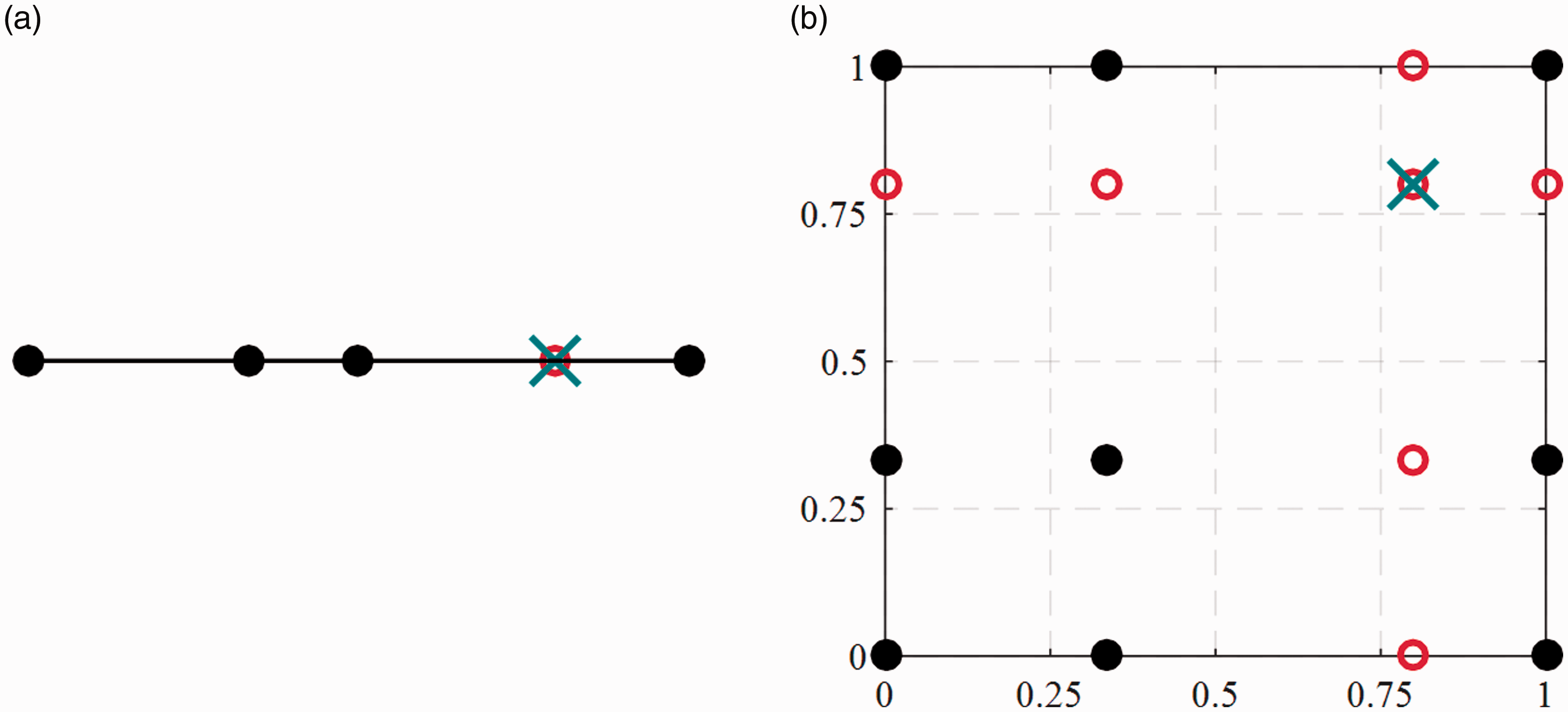
The adaptive PMOR approach proposed in previous sections is subsequently illustrated with its application to the moving coil of electrical-dynamic shakers. Because the geometric model has perfect cyclic symmetry property, it can be simplified to one over 16 of the entire model as shown in Figure 2. The finite element model consists of 15,608 SOLID elements and 21,246 nodes. The number of the full DOFs is 59,487.

Figure 2.

The moving coil of electrical-dynamic shakers: (a) the entire geometric model; (b) the simplified FE model.

First, we import the simplified geometry model into HYPERMESH and generate the original regular mesh. Then we utilize the HYPERMORPH module to parameterize the mesh without changing the underlying topology. Several FE models corresponding to the initial parameter sets are generated, respectively. Their nodes coordinates are exported for the use of generation of new FE model in ANSYS. The boundary condition and excitation condition are also initialized in HYPERMESH. At the position shown in Figure 2(b), only axial displacement is permitted, and the normal displacement at the symmetric boundary is zero. The model is excited by 1 g base acceleration imposed on the drive coil.

The sampling scheme is automatically implemented in MATLAB including calling ANSYS to generate FE model and corresponding matrices, reading the matrices files, and conducting the classical and proposed adaptive PMOR methods.

This research is applicable to multi-dimensional cases. In this application, we consider a two-dimensional parameter space, which is spanned by the thickness of stiffener plates T, changing from 10 to 32 mm, and the radius of the table R, changing from 460 to 510 mm. The original parameter configuration is T = 18 mm and R = 485 mm.

Three different offline sampling procedures and ROMs generation methods are compared. The first one is the classical procedure outlined in Algorithm 1 in which the candidate set is uniformly selected (referred to as “Uniform + Krylov”). A modified Arnoldi algorithm ¹⁸ is applied to build the 30-order basis spanning the Krylov subspace. The second one is a variation of the classical algorithm in which the ROBs are built by 20-order orthogonal eigenvectors after a Gram–Schmidt process (referred to as “Uniform + Modal”). The third approach is the proposed adaptive procedure summarized in Algorithm 2 (referred to as “Adaptive + Modal”). The random candidates are selected by Latin hypercube sampling. The maximum number of random candidates is set to Nc = 30 for the adaptive procedure.

The performance of each approach is assessed by monitoring the maximum errors of frequency, modal shape, and response between the HDM and interpolated ROM. As the iteration increases, the number of corresponding parameter sampling points grows exponentially. With four initial points, a total of 49 parameter samples are added after six iterations.

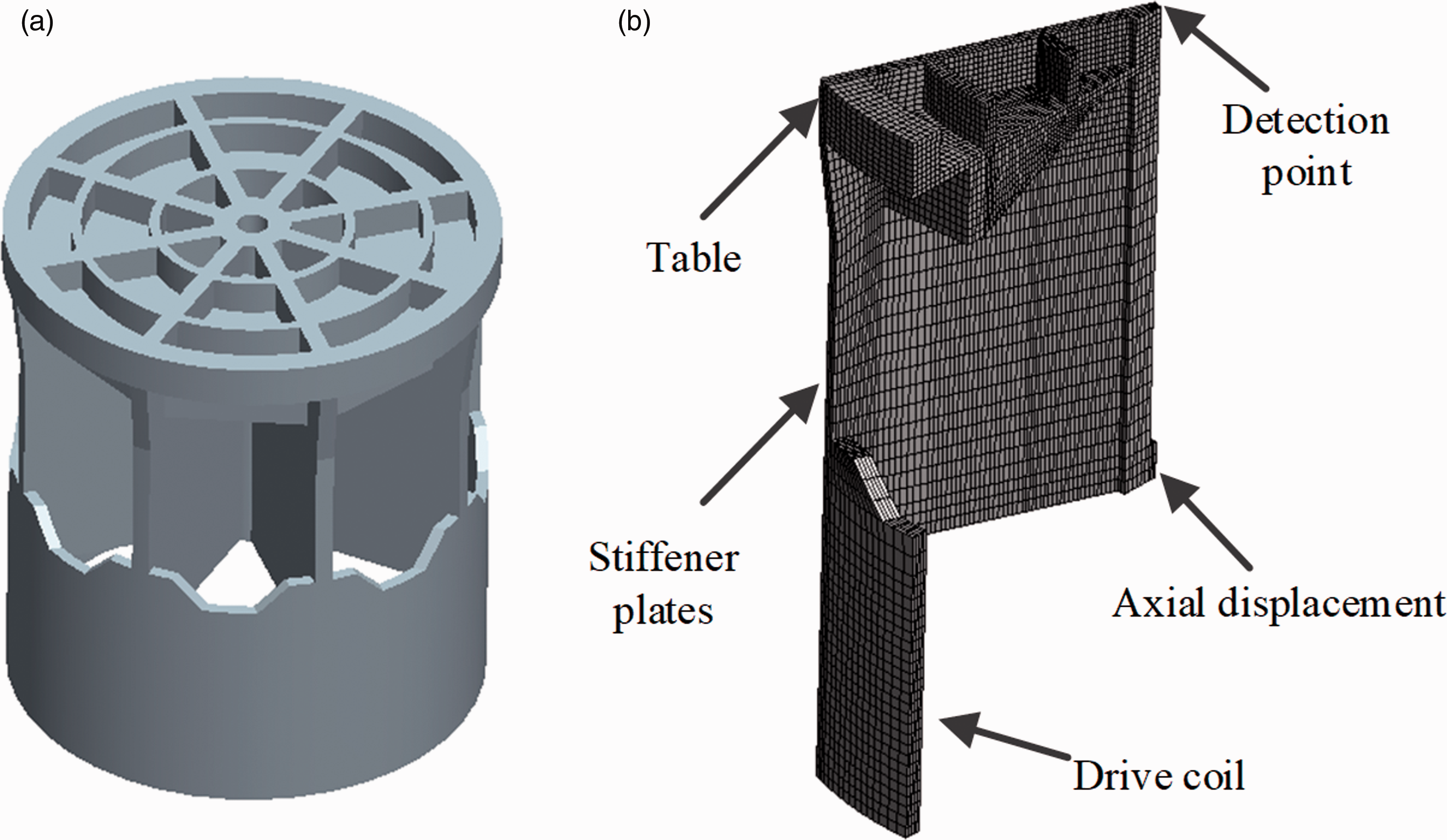
Figure 3 reports the evolution of the maximum errors. It can be observed that the maximum errors decrease a lot as the parameter sample points increase. Compared with frequency, the modal shape and response have larger errors and consequently can be used as the most rigorous criteria. In other words, once the error of modal shape or response match the specified tolerance, the underlying model should be accurate enough.

Figure 3.

Error evolutions for different PMOR methods. (a) Frequency, (b) Modal shape and (c) Response.

One can also observe the superiority of the modified ROB over the regular Krylov-subspace based ROB. Take the errors of response for example, with the same 49 evenly distributed sample parameters, the PMOR approach with classical Krylov ROBs can only decrease the maximum relative error from 4.72 to 0.11%. While the one with modified modal ROBs achieves an asymptotic error of 0.007%. It means that the sampling approach can reach the same level of maximum error with fewer sample points by use of modified ROBs.

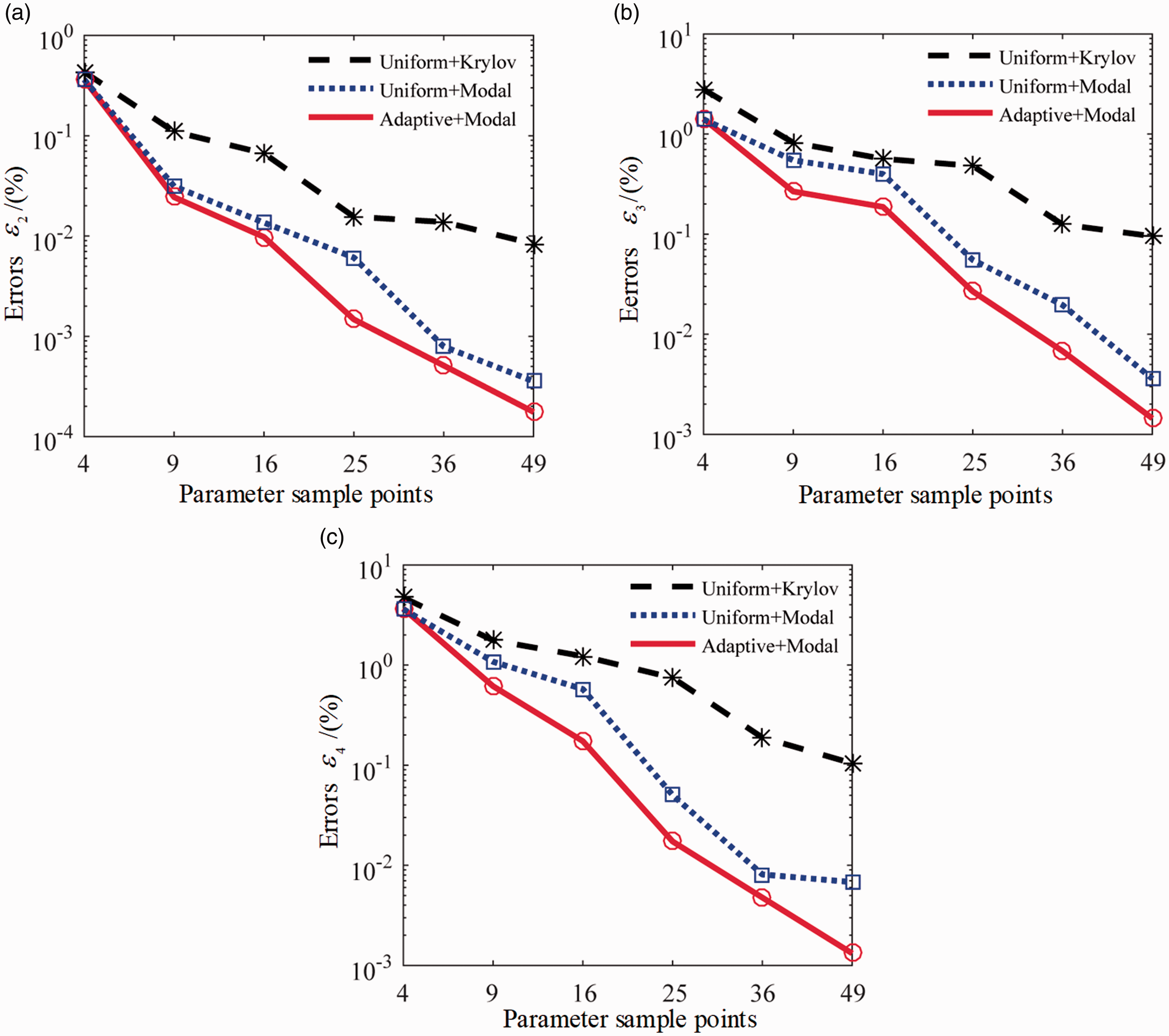
In contrast, the adaptive approach achieves a smaller error of 0.0013%. As a matter of fact, the adaptive approach outperforms the modified classical method in all the three errors, with the frequency error decreasing from 3.56 × 10⁻⁴ to 1.76 × 10⁻⁴%, the modal shape error from 0.0036 to 0.00144%, and the response error from 0.0068 to 0.0013%, after 49 points sampled. Compared with the uniform sampling procedure, the adaptive approach is more suitable for the models with relatively strong parameter dependency at a certain area of the parameter space. In this application, the proposed sampling procedure captures the nonlinear parameter dependence in the dimension of table radius R and refines the corresponding area adaptively, thus leading to more accurate PROMs. The final uniform and adaptive sample grids are shown in Figure 4. The parameter domain is normalized to [0, 1] × [0, 1] for the sake of an easier presentation.

Figure 4.

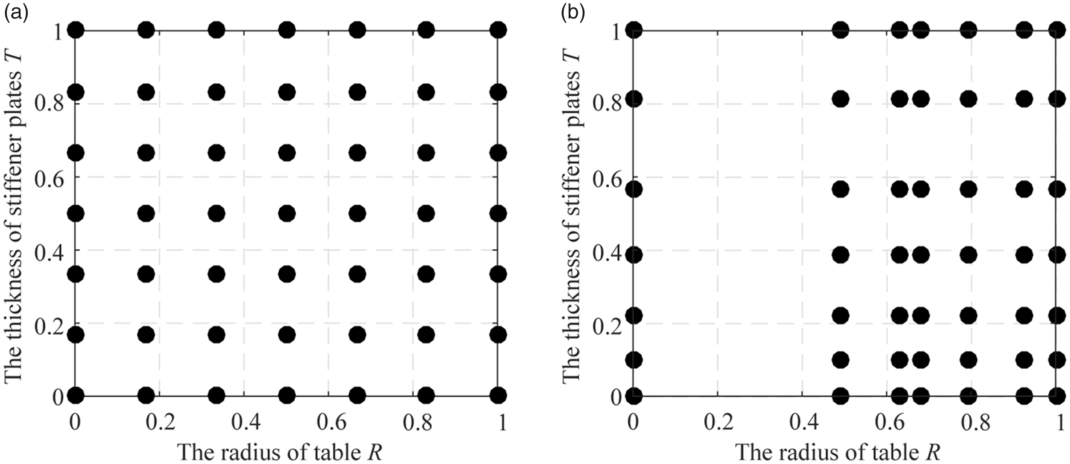
The final parameter samples of uniform and adaptive methods: (a) uniform method; (b) adaptive method.

In order to comprehensively evaluate the performance of the proposed methods, we compare the calculation time of the three algorithms and present the results in Figure 5. As for the uniform sampling methods, the distribution of the parameter samples changes as the iteration increases. Therefore, the calculation time of the final iteration with 49 samples is considered. The total time includes FE model generation and reduction time, together with the extra exploration time for the adaptive procedure.

Figure 5.

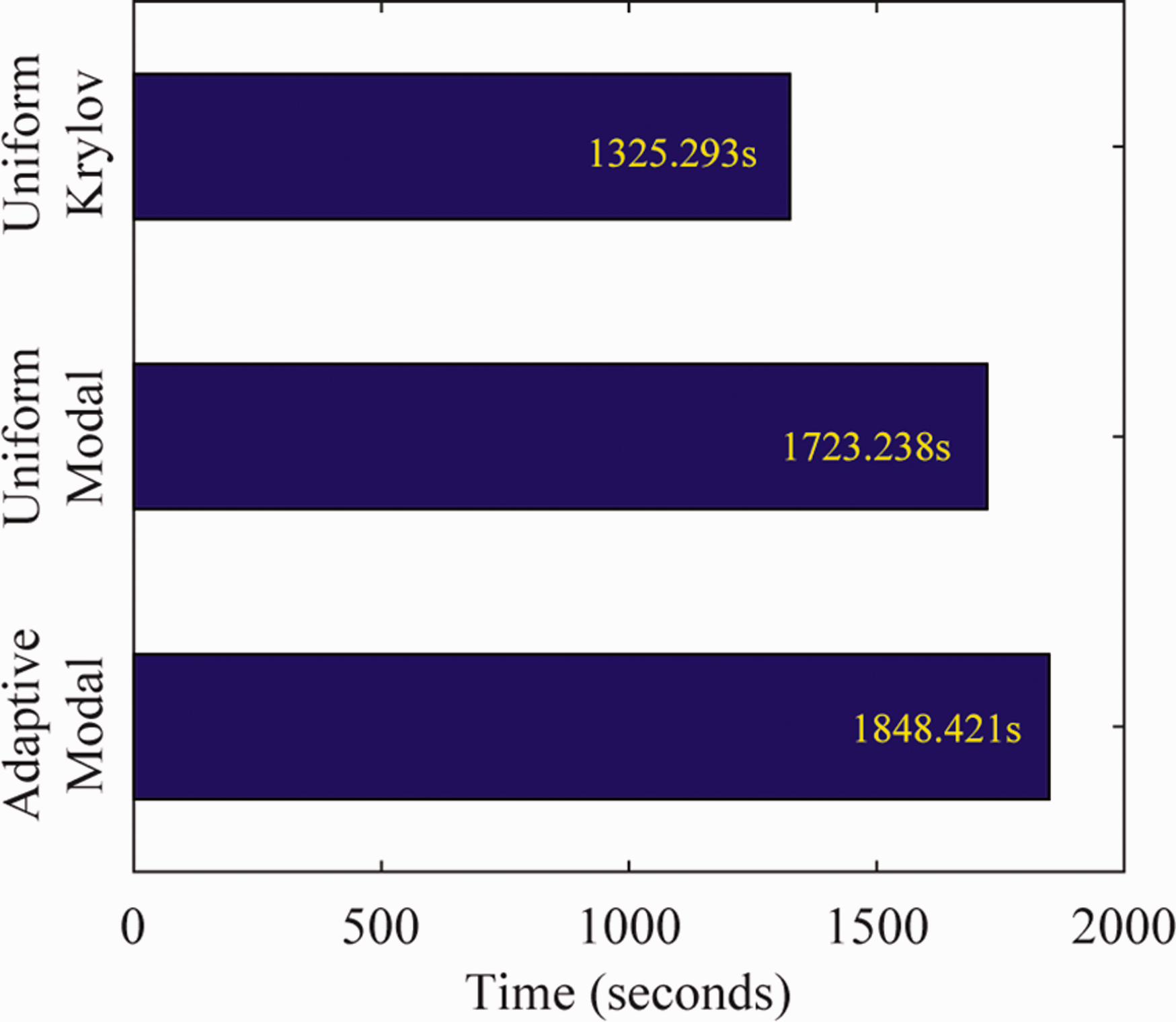
The calculation time of the three algorithms.

As shown in Figure 5, costs for the two modal basis-based approaches are comparable, which implies that the adaptive procedure carries no much extra computational cost compared with the uniform sampling method. While the calculation time of Krylov subspace-based method is nearly one-quarter smaller than its counterpart computed with modal basis. This is due to the fact that computing the eigenvectors requires more computational resources than calculating the Krylov basis. However, the modal basis could provide more accurate ROMs compared to the latter.

The convergence performance of the proposed approach is also considered. There is no guaranty that adding a parameter sample point will necessarily lead to a monotonic decrease of maximum errors. But in practice, the maximum error will decrease for most additional sample points due to the convergence property of Lagrange interpolation method exploited in our approach.

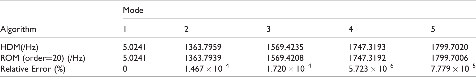
Furthermore, in order to validate the error indicator and display the intuitionistic comparison between the HDM and ROM constructed with adaptive PMOR approach, we compare the first five orders frequencies and the fourth-order modal shape after seven parameter points have been sampled. The query point is T = 24.93 mm and R = 472.44 mm at which the error indicator reaches the maximum.

It should be noted that these results are presented to validate the proposed PMOR method, not to illustrate the superiority. Therefore, the results of classical PMOR method are not included.

The results shown in Table 1 and Figure 6 reveal that the interpolated ROB after six sampling iterations is capable of reproducing very accurately the HDM solution with almost negligible errors.

Table 1.

Comparison of nature frequencies between HDM and ROM.

Algorithm	Mode
	1	2	3	4	5
HDM(/Hz)	5.0241	1363.7959	1569.4235	1747.3193	1799.7020
ROM (order=20) (/Hz)	5.0241	1363.7939	1569.4208	1747.3192	1799.7006
Relative Error (%)	0	1.467 × 10–4	1.720 × 10–4	5.723 × 10–6	7.779 × 10–5

Figure 6.

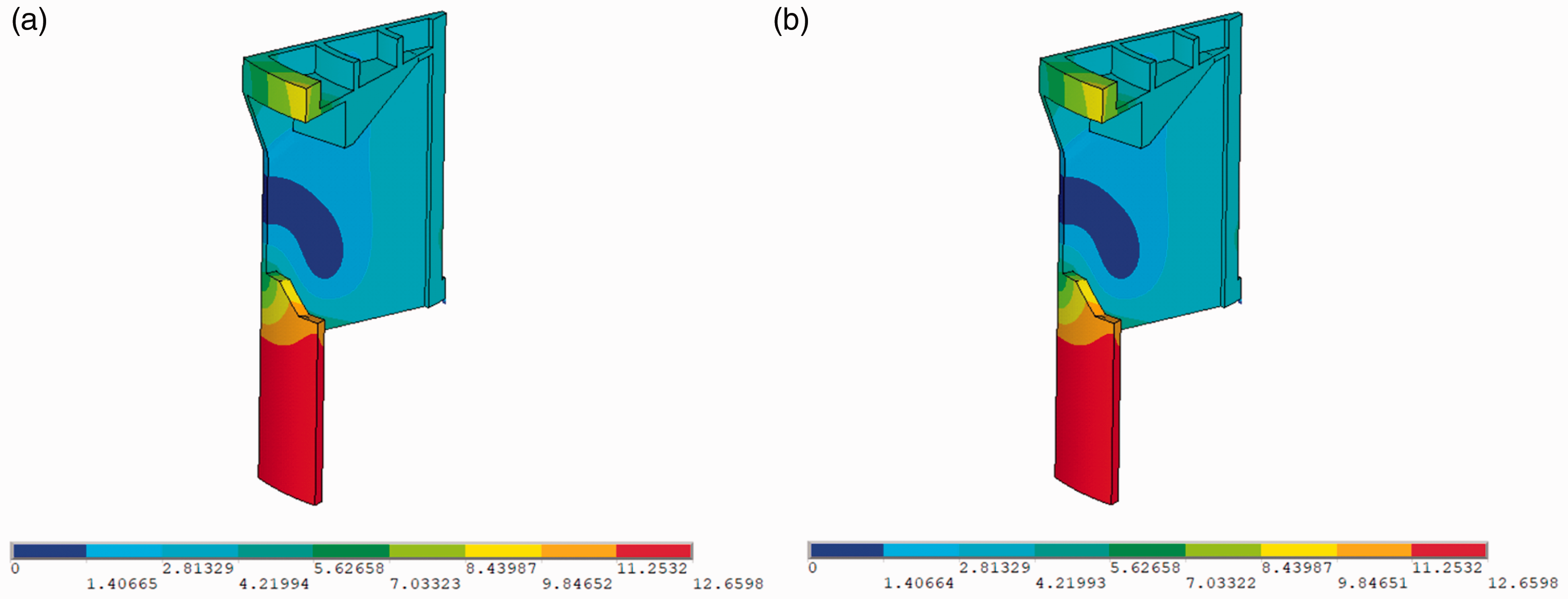
Comparison of the second order modal shape between HDM and ROM: (a) HDM and (b) ROM.

The harmonic response for the HDM and ROM is subsequently compared in the frequency range of 0–1850 Hz with the interval 0.1 Hz. The detecting point locates at the center of top surface as shown in Figure 2(b). Rayleigh damping coefficient is adopted in the harmonic response analysis (α= 2.5, β = 9 × 10⁻⁵). For clarity, the results between 0 and 1550 Hz are plotted using a base 10 logarithmic scale for the x-axis and a linear scale for the y-axis as shown in Figure 7(a). While for the range of 1550–1850 Hz, linear scales are used for both the x-axis and y-axis as shown in Figure 7(b).

Figure 7.

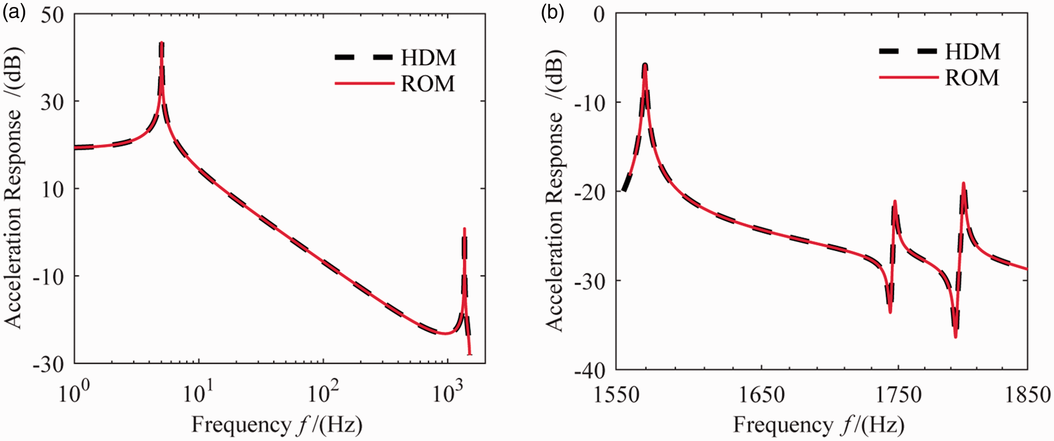
Comparison of harmonic responses between HDM and ROM: (a) frequency range: 0–1550 Hz; (b) frequency range: 1550–1850 Hz.

As illustrated in Figure 7, the harmonic response predicted by the ROM is almost indistinguishable from its HDM counterpart. A perfect level of accuracy is observed in the full frequency range, validating the proposed framework.

To investigate exact errors and assess the accuracy of these PROMs, the first five orders resonance responses are compared in Table 2.

Table 2.

Comparison of resonance responses between HDM and ROM.

Algorithm	Mode
	1	2	3	4	5
HDM (/dB)	43.8517	0.8156	–5.8489	–21.1953	–19.0978
ROM (order=20) (/dB)	43.8517	0.8157	–5.8487	–21.1957	–19.0975
Relative Error (%)	0	1.226 × 10–2	3.419 × 10–3	1.887 × 10–3	1.571 × 10–3

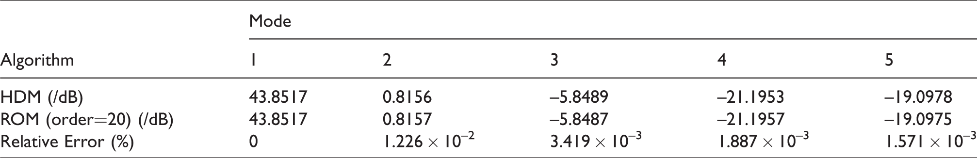
The results reported in Table 2 reveal that the relative errors are below 0.02%, and very good predictions are obtained with the ROM. It indicates that the proposed adaptive PMOR procedure can be exploited to generate high-precision surrogate ROMs for fast simulation of the complex FE models.

Conclusions

This paper presents an automatic adaptive sampling procedure for PMOR by matrix interpolation. The procedure is based on the definition of error indicator developed in this research as a measure of the need for a new sample point. The proposed approach combines the benefits of matrix interpolatory PMOR and those of adaptive sampling parameters procedure. The outlined scheme can be applied to the models with arbitrary parametric dependency and can adaptively determine the minimum parameter sample points to satisfy the predefined error. In addition, by utilizing the orthogonal eigenvectors as the ROB, this approach shows great superiority over the classical PMOR method. Numerical experiments illustrate that the ROM can provide perfect predictions of frequencies, modal shapes, and responses. This automatic adaptive method can be used for order reduction of realistic complex FE models.