Stacked sparse autoencoder in cavitation noise signal data classification of hydro turbine based on power spectrum

Abstract

Cavitation is a phenomenon that occurs during the continuous operation of a hydro turbine that directly affects the efficiency and working capacity of the unit. This paper proposes an innovative classification paradigm that uses deep learning-based methodologies in order to identify both cavitation noise signal and non-cavitation noise signal that will help prevent the damage or breakage in the earliest possible time to avoid more irreversible and irreparable damage to the hydro turbine. The stacked sparse autoencoder (SSA) nuclear framework is utilized to learn more abstract and invariant high-level features from the multiple feature sets. Then, the method on minimum redundancy maximum relevance (mRMR) selection is used to evaluate and sort out all the characteristics found by the stacked sparse autoencoder. Finally, the random forest (RF) classifier algorithm is employed to perform supervised fine-tuning and classification. The traditional supervised learning models such as support vector machine, logistic regression, and sparse representation classification are chosen to be used as contrast algorithms. SSA-mRMR-RF generally produces a better performance than the support vector machine, logistic regression and sparse representation classification when used in the same set of features. The SSA-mRMR-RF produced the highest overall average accuracy since it reached 93.18%. The SSA-mRMR-RF offers a 3.85% higher overall accuracy than the support vector machine. It also offers a 2.44% higher overall accuracy than logistic regression. In addition, it also offers a 20.30% higher overall accuracy than the sparse representation classification on the average. When the signals are divided into three categories, the highest overall accuracy decreased to 71.88%, and the classification accuracy of incipient noise signals is very low. Therefore, this paper proposes the models of power spectral-SSA-mRMR-RF and fast Fourier transform-SSA-mRMR-RF to be used, and these discoveries are based on the frequency characteristics of the cavitation noise signal. The highest overall accuracy rebound went back to 88.97% based on the power spectrum, and 96.05% based on fast Fourier transform. The corresponding experimental results found on the four data sets of the different operating conditions demonstrate that the proposed methods for discovering the extent of cavitation outperforms these traditional alternatives.

Introduction

As the years pass, electrical power or energy has always been in great demand. And because of the diversification of industrial and domestic power consumption in large cities, the stability of power supply, power generation capacity, as well as power generation methods has attracted constantly increasing attention. ¹ People realized that constructing a safe, economical, and clean electric power system is essential and indeed significant for the sustainable development of the human society. ² Nowadays, global energy crisis and environmental pollution problems have already adversely affected human lives. Therefore, since it is the most mature and reasonable source of clean energy in both technology and economy, hydroelectric power generation has received great attention and utilization. The cavitation of the hydro turbine is the most important factor that affects the efficiency of hydropower generation and the safety of the energy or power generating units. ³ During the continuous rotation in a hydro turbine operation, if serious cavitation occurs, the stability of the water body that passes will be changed and the rotation of the turbine will be affected. This will definitely result in severe vibration of the turbine; then the operating efficiency of the turbine will be greatly reduced. If severe cavitation frequently happens, cavitation erosion will occur on turbine blades. ⁴ If the maintenance of these turbine blades is not regular and timely, it will cause serious accidents. So, it is particularly essential to monitor the degree of cavitation on the turbine. Because the turbine blades are located in a closed spiral case, ⁵ difficulties are always present in monitoring the cavitation state of the turbine. This is why it is very important to study the cavitation of the hydro turbine before it becomes inefficient in generating essential energy.

Currently, more and more researchers are trying to solve the problem of cavitation by using a variety of methods. Ghorbani et al. ⁶ presented visualization and image processing of the spray structure affected by cavitation bubbles and cavitating flow patterns. They tried to find the extent of cavitation through the image in order to generate a better understanding of cavitation as well as the resulting flow regimes. This attempt cannot fundamentally solve the problem regarding the reduction of unit efficiency which was caused by cavitation. Also, this type of processing can only be done in the laboratory, and it cannot be used in an actual hydropower station. This is because of the location of the turbine which is always in an airtight volute, and it is really impossible to take a photograph or even acquire a clear image. On the other hand, Grewal et al. ⁷ attempted to reverse cavitation erosion by utilizing surface modification techniques. In their study, a novel attempt has been made to modify the surface properties of the hydro turbine steel with the aid of friction stir processing. By using this method, processed steel became harder by 160% in comparison to unprocessed steel. It was realized that this method can only delay the corrosion time of turbine blades. It does not take into account the problem on the generation efficiency reduction when cavitation occurs, and it also requires a large amount of cost. Roy ⁸ proposed a method to identify the pressure field that could generate individual pits, as observed experimentally on eroded samples of Aluminum alloy 7075-T651. This method gives access to the load distributions, relevant to the flow aggressiveness of the cavitation test. This research focuses on the damage on the wheel blades caused by cavitation. In our case, our ultimate goal is to adjust the operation conditions of the hydraulic turbines before cavitation becomes very serious, reduce the intensity of cavitation, improve the efficiency of the operation of the hydro turbines, and delay the process of wheel loss. So, our proposal is more on prevention and extending the work life of the hydro turbines.

Cavitation noise detection is an effective method for investigating cavitation caused when bubbles generate, collapse, and rebound and these usually accompany the noise. Analyzing the cavitation noise signals can assist in finding the cavitation characteristics. The conventional power spectrum analysis of an acoustical measurement is normally employed for an inception criterion.^9,10 It was realized that the presence of increase within a certain frequency band of the power spectrum in comparison with a non-cavitation condition can be a sign when the cavitation happened. Lee et al. employed the short-time Fourier transform analysis and the Detection of Envelope Modulation On Noise spectrum analysis, both of which are appropriate in finding such a repeating frequency. This approach can be practical if the acoustical signature is pre-identified in various cavity patterns, which is not true in the majority of cases. In addition, when the work environment becomes complicated, the structure of the equipment becomes more and more complex; therefore, it can be confusing to detect the cavitation phenomenon. ¹¹

Noise classification is an issue of great significance when it is used to detect the cavitation noise. ¹² Jiang et al. first put forward the method of classification algorithm used to identify the cavitation noise signal and the non-cavitation noise signal during the academic conference of the third International Conference on Computer Science and Network Technology. By using the support vector machine (SVM) to distinguish both the cavitation noise signal and the non-cavitation noise signal, the recognition rate is 81.24%, a near-perfect result. But when you add the incipient-cavitation noise signal, the recognition rate of this method is poor.

This paper proposes an innovative classification method for cavitation noise signal by using deep learning-based methodologies. First, the stacked sparse autoencoder (SSA) is utilized to learn the more abstract and invariant high-level features from the multiple feature sets. Then, the method of minimum redundancy maximum relevance (mRMR) algorithm is used to evaluate and sort all the characteristics found by the SSA. Finally, the random forest (RF) classifier is employed to perform supervised fine-tuning and classification. The traditional classification method such as SVM, logistic regression (LR), and sparse representation classification (SRC) are chosen to be used as the contrast algorithm.

The uniqueness of this method is that, after the stacked sparse autoencoder is used to find the characteristics of the signals by aiming at the complex characteristics of the hydro turbine cavitation noise signal, then a feature selection process is added, and the RF classifier is used to sidestep the appearance of the local optimum phenomenon. The method proposed in this paper can clearly identify the occurrence of cavitation more effectively, and then guide the hydroelectric power station when to adjust its operating conditions (OCs) in time. This will help reduce the impact of cavitation erosion on the blades, improve the operation efficiency of the turbine and consequently save a substantial amount in the maintenance and repair cost of the hydroelectric power station.

Methodologies

Sparse autoencoder and SSA

A deep learning (DL) network method learns multilayer features by stacking unsupervised modules on top of each other. One of the major branches of DL models is sparse autoencoder (SA); it is a bioinspired hierarchical neural network that has an intrinsic ability to extract more abstract features from the data which contains one input layer, one hidden layer, and one reconstruction layer. Commonly, the previous layer of neurons is connected to the next layer of neurons, but no connections exist among the same layer of neurons. ¹³

Basically, a shallow autoencoder consists of two steps: these are encoding and decoding, comprised of one visible layer, one hidden layer, and one reconstruction layer as shown in Figure 1. In the encoding stage, the autoencoder is able to give a concise representation of the input through connections between the input and hidden nodes. In the decoding stage, the autoencoder aims to reconstruct the input from the extracted feature representation in an unsupervised pattern. To this end, the DL model is able to learn a concise representation of the input, given that the number of hidden neurons is less than the dimension of raw input.

Figure 1.

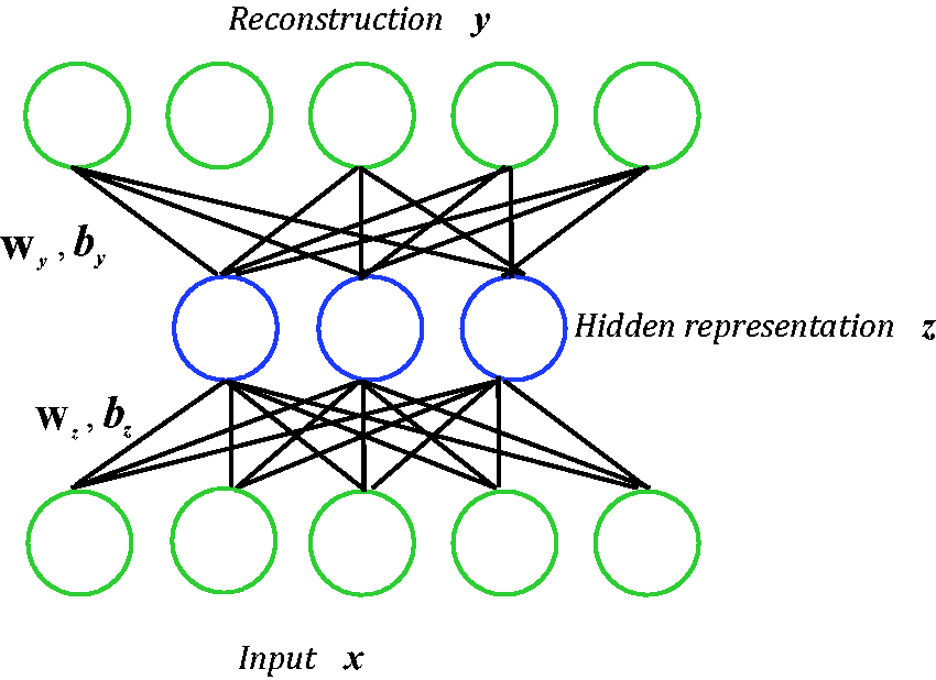
Schematic diagram of single-layer autoencoder architecture.

In addition, in the autoencoder framework, neurons between two adjacent layers are completely connected and trained, which means that the neurons in the previous layer are beneficial to the nodes in the next layer. In this way, the DL network needs to train a lot of parameters. This results to a considerable amount of time to optimize the parameters and is considered as an undesirable factor. To address this issue, a biologically inspired autoencoder model is first introduced into the data classification, which is performed by employing the LRF（local receptive field） concept in neuroscience. A locally dense connection instance of two adjacent layers is shown in Figure 2, where the connections of neurons between a previous layer and a subsequent layer are randomly produced according to some conditional probability distributions. Concretely, the major intention of the local receptive field-based autoencoder is to conduct a locally dense connection between the previous layer and the next layer. This strategy is promising since it can further enhance the classification performance and reduce the training time, compared with the fully connected autoencoder architecture.

Figure 2.

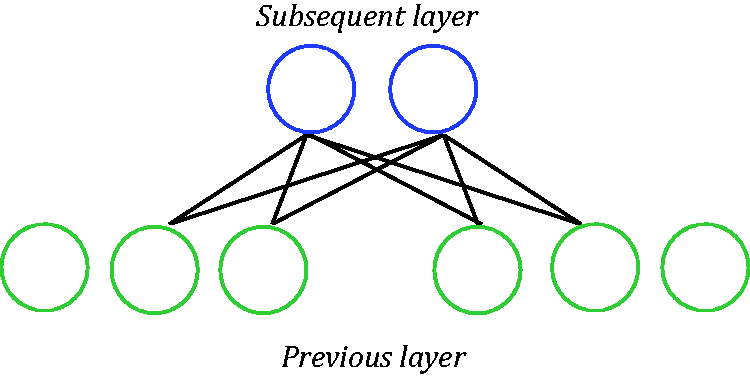
A locally dense connection instance of neurons between the previous layer and subsequent layer.

During training, the encoder of SA which transforms the input vector $\mathit{x}\in {\Re }^D$ into the hidden representation $\mathit{z}\in {\Re }^S$ by linear mapping and a nonlinear activation function, and $\mathit{z}$ can be considered as a new feature representation of the raw input

$$\mathit{z}=f({\mathbf{W}}_{\mathit{z}}\mathit{x}+{\mathit{b}}_{\mathit{z}})$$

(1)

Here, $D$ is the dimension of input data and $S$ is the number of hidden neurons, ${\mathbf{W}}_{\mathit{z}}\in {\Re }^{S\times D}$ 、 ${\mathit{b}}_{\mathit{z}}\in {\Re }^{S\times 1}$ represent the weight matrix and offset vector of the input layer to the hidden layer, respectively. The logistic sigmoid function $f(x)={(1+\exp (-x))}^{-1}$ is used in the encoding and decoding structures. The obtained hidden representation $\mathit{z}$ is further mapped to reconstruct an approximation of the $\mathit{y}$ value of the raw input using a decoding function

$$\mathit{y}=f({\mathbf{W}}_{\mathit{y}}\mathit{z}+{\mathit{b}}_{\mathit{y}})$$

(2)

Where ${\mathbf{W}}_{\mathit{y}}$ is a $D\times S$ decoding matrix and ${\mathit{b}}_{\mathit{y}}$ is the offset vector of dimensionality $D$ . By employing the back-propagation algorithm, features in the data are extracted by minimizing the difference between input and its reconstruction. Then the features are encapsulated in the weight matrix $\mathbf{W}$ and bias vector $\mathit{b}$ . To fulfill this, the objective function of the SA architecture with a weight decay term and a sparsity constraint term is defined as

$$J_{\mathrm{SA}}(\mathbf{W},\mathit{b})=\frac{1}{\mathrm{M}}{\displaystyle \sum _{i=1}^{\mathrm{M}}\left(\frac{1}{2}{\Vert {\mathit{y}}_i-{\mathit{x}}_i\Vert }_2^2\right)}+\frac{\lambda }{2}{\displaystyle \sum _l{\displaystyle \sum _i{\displaystyle \sum _j{\left(W_{i,j}^{(l)}\right)}^2}}}+\eta {\displaystyle \sum _{j=1}^S\mathit{KL}(r||{\overline{r}}_j)}$$

(3)

where $\lambda$ is a weight decay parameter, and $W_{i,\hspace{0.17em}j}^{(l)}$ stands for the connection between the ith neuron in layer $l-1$ and the jth neuron in layer $l$ ; $\eta$ is the weight of the sparsity penalty; $r$ is the sparsity parameter with a small proper value; and ${\overline{r}}_j$ is the average activation of the hidden unit $j$ . Moreover, $\mathit{KL}(r\text{||}{\overline{r}}_j)$ is a Kullback-Leibler divergence between $r$ and ${\overline{r}}_j$

$$\mathit{KL}\left(r\left|\right|{\overline{r}}_j\right)={\displaystyle \sum _{j=1}^S\left(r\log \frac{r}{{\overline{r}}_j}+(1-r)\log \frac{1-r}{1-{\overline{r}}_j}\right)}$$

(4)

The cost function $J_{\mathrm{SA}}(\mathbf{W},\mathit{b})$ with parameters $\theta =\{{\mathbf{W}}_{\mathit{z}},{\mathbf{W}}_{\mathit{y}},{\mathit{b}}_{\mathit{z}},{\mathit{b}}_{\mathit{y}}\}$ can be optimized via stochastic gradient descent algorithm and backpropagation algorithm. Afterwards, $J_{\mathrm{SA}}(\mathbf{W},\mathit{b})$ is expected to produce a considerably small value which prompts the SA to learn abstract features from the original data by using a forward passing step.

The SSA is a layer-wise encoding neural network in which multiple layers of shallow sparse autoencoders are stacked up, which can then be pre-trained via greedy methods layer by layer. ¹⁴ An example of a SSA architecture which consists of two basic SA is shown in Figure 3, where the decoder parts of each SA is not provided for simplicity. Commonly, this stacked network can be illustrated by the following steps: first, a SA on the raw input $\mathit{x}$ is trained to learn the first-order feature representation ${\mathit{z}}^{(1)}=f_{{\theta }_1}(\mathit{x})$ . Then, the low-level representation ${\mathit{z}}^{(1)}$ is fed as the “original input” into the next shallow SA for extracting the second-order feature representation ${\mathit{z}}^{(2)}=f_{{\theta }_2}(\hspace{0.17em}{f}_{{\theta }_1}(\mathit{x}))$ . Following this, the lth level representation ${\mathit{z}}^{(l)}=f_{{\theta }_l}(\hspace{0.17em}{f}_{{\theta }_{l-1}}(\dots f_{{\theta }_1}(\mathit{x})))$ can be learned by a recursive forward propagation learning rule. Finally, to achieve a better classification performance, a RF classifier is employed to further fine-tune the whole pre-trained network and determine the corresponding class label for each sample.

Figure 3.

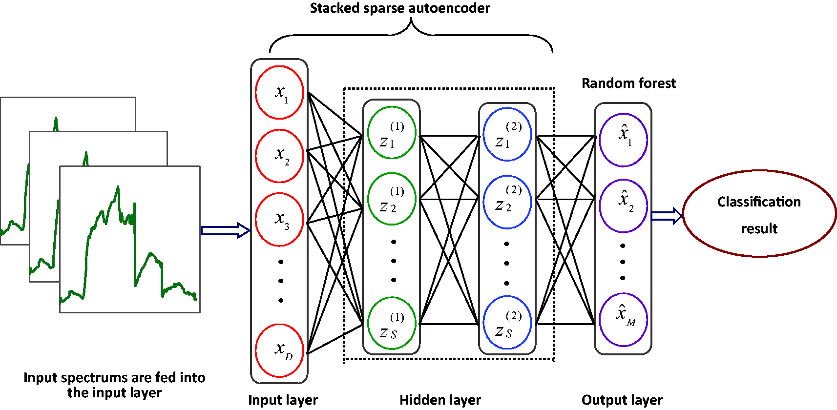
A stacked sparse autoencoder connected with a random forest classifier for data classification.

Feature selection based on mRMR

If we input all the cavitation noise characteristics obtained by the SSA into the classifier for recognition, the recognition efficiency and accuracy will be reduced. Therefore, we need to find a suitable evaluation index to evaluate and sort all the characteristics found. The method of mRMR uses the correlation between the information as an evaluation index, which can then find the optimal characteristic subset. ¹⁵

Assuming that an m-dimensional fault sample space with $c$ fault characteristics and $n$ fault samples, the mRMR can select an optimal subsample space $S$ with p-dimension $(p\le m)$ from the original sample space. In the subsample space S, the redundancy of repeated information between each fault feature is the smallest, and the correlation between the features and the faults is the largest.

$p(x)$ and $p(y)$ are defined as the probability of $X$ and $Y$ . $p(x,y)$ is the joint probability of $X$ and $Y$ . $I(X;Y)$ is defined as the mutual information of $X$ and $Y$

$$I(X;Y)={\displaystyle \sum _{x\in X}{\displaystyle \sum _{y\in Y}p(x,y)\log \frac{p(x,y)}{p(x)p(y)}}}$$

(5)

$I(X;c)$ is defined as the mutual information between the feature $x_i$ and the fault class $c$ in the subspace feature $S$ . Then the principle of maximum relevance is defined as

$$\max \hspace{0.17em}D(S,c),D=\frac{1}{\left|S\right|}{\displaystyle \sum _{x_i\in S}I(x_i;c)}$$

(6)

where $\left|S\right|$ is the dimension of characteristic space. $I(x_i;x_j)$ is defined as the mutual information between the feature $x_i$ and the feature $x_j$ in the subspace feature $S$ . Then the principle of minimum relevance is defined as

$$\min R(S),R=\frac{1}{{\left|S\right|}^2}{\displaystyle \sum _{x_i,x_j\in S}I\left(x_i;x_j\right)}$$

(7)

Equations (8) and (9) are the feature evaluation criteria of mRMR, which is defined as

$$\max \Phi (D,R),\Phi =D-R$$

(8)

$$\max \Phi (D,R),\Phi =D/R$$

(9)

Equations (10) and (11) are mutual information gap standards and mutual information quotient standards. In the process of optimization, the incremental optimization algorithm is used to get the optimal subset of the fault features, thus realizing the feature optimization. Supposing that $k-1$ features have been selected, and the feature subspace $S_{k-1}$ has been constructed, the following criteria should be followed when selecting the kth feature from the remaining feature space $\left\{X-S_{k-1}\right\}$

$$\underset{x_j\in X-S_{k-1}}{\max }\left[I(x_j;c)-\frac{1}{k-1}{\displaystyle \sum _{x_i\in S_{k-1}}I\left(x_j;x_i\right)}\right]$$

(10)

$$\underset{x_j\in X-S_{k-1}}{\max }\left[I(x_j;c)/\frac{1}{k-1}{\displaystyle \sum _{x_i\in S_{k-1}}I\left(x_j;x_i\right)}\right]$$

(11)

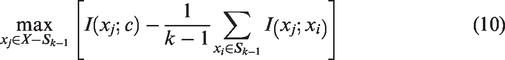
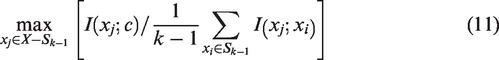
When there is need for a new feature to be selected, after some features have been selected, the remaining features need to be recalculated according to equations (10) and (11). And then, the feature which satisfied the two conditions of equations (10) and (11) can be selected as the next feature.

In this paper, a feature selection algorithm based on the mRMR is used to find the optimal feature subset, which was then used as the input into the classifier for training and testing, so as to realize the recognition of cavitation noise types.

RF classifier

The RF classifier is a soft classifier of decision tree-based ensemble methods. ¹⁶ The model is a majority vote mechanism of decision tree predictors where each tree is formed by using the resampling technique with replacement. Consequently, the different subsets from the original training sets are adopted to form each tree (in-bag set). Meanwhile, the remaining subset is used in the decision tree to construct a test classification (out-of-bag set). Furthermore, the best splits are selected among random subsets of the predictor variables, where a terminal node occurs. To classify the out-of-bag dataset in the RF classifier, the vector is run down in each of the trees in the forest. Finally, the assignment of class label of an unknown instance is then determined by a majority vote. Basically, the RF algorithm is based on the Gini index minimum principle, and the Gini index is described by

$$\mathit{Gini}(s)={\displaystyle \sum _{i=1}^K{p}_{n_i}}\left(1-p_{n_i}\right)$$

(12)

where $K$ is the number of classes, and $P_{n_i}$ is the probability of being classified into the corresponding land cover class $n_i$ at node $s$ , is defined as

$$p_{n_i}=\frac{l_{n_i}}{l}$$

(13)

where $l_{n_i}$ is the number of trees belonging to class $n_i$ , and $l$ is the total number of classification trees.

There are several reasons why the RF is regarded as one of the most successful tree-based ensemble tools for classification better than the traditional softmax classifier: (1) the RF method can effectively handle the problems caused by dimensionality and it helps avoid over-fitting the model with less sensitivity toward noisy data; (2) RF can produce an unbiased data imputation mechanism when prediction trees are correlated, and this can effectively determine a nonlinear model between the predictors and the outcomes of interest; and (3) the RF has hardly any parameters to adjust, thereby assisting in having minimized assumptions of the dataset.

Experiments on cavitation noise signal

In this paper, an innovative classification method for capturing cavitation noise signal using DL-based methodologies is proposed. First, the SSA is utilized to learn more abstract and invariant high-level features from the cavitation noise signals. Second, mRMR is used to evaluate and sort all the characteristics found by the SSA. Afterwards, the secondary characteristics are discarded, and then the important features are transported to the RF classifier to perform supervised fine-tuning and classification.

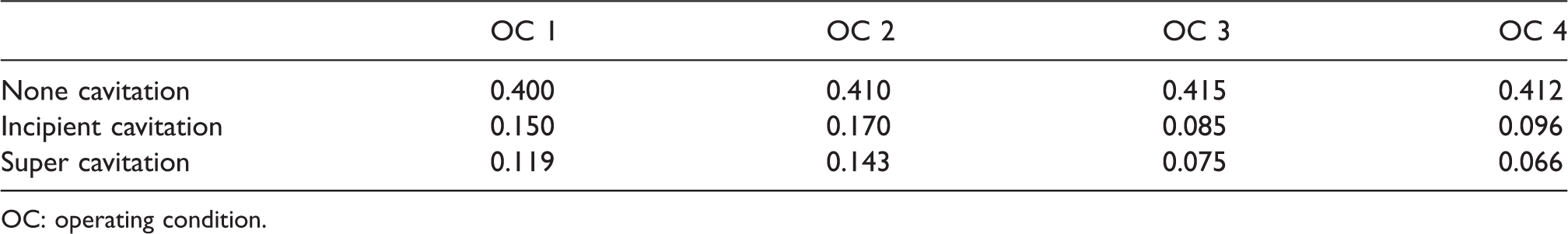
The data in this paper were obtained from the hydraulic turbine model test bench of Harbin electric machine factory. Here, we chose a total of four different OCs. In each of the operating conditions, when the unit started to run, we adjusted the $\sigma$ by controlling the pressure of the draft tube. This was done by using the stroboscope to monitor the occurrence of non-cavitation, incipient cavitation, and super cavitation. Then, we used the hydrophone to collect the mixed acoustic signal. We chose about 15 monitoring positions (different values of $\sigma$ ) to record the data for about 10 s in every operating conditions repeatedly. The monitoring positions near the incipient cavitation should be chosen more in order to find the different characteristics of the incipient cavitation from the others.

A set of experiments composed of the cavitation noise signal data collected from four different operating conditions is performed to evaluate the effects of the different number of training samples to the classification approaches, and this is regarded as a critical variable in the classification tasks. To this end, the training size is changed from 5% per class to 25%, and the remaining samples as testing ones. The average overall accuracies for the different classification approaches with the different number of training samples are shown in Figure 4. It is clear that the performances of the proposed method and other approaches compared gradually improved with the increase of training samples except for the SRC. When the percentage of the training size of SRC method is increased, the overall accuracy (OA) went up and down and did not monotonically increase. When the percentage of the training size is increased from 20% to 25%, the increase in the OA is not obvious; there were even times when the OA decreased. Therefore, choosing 20% of the training size of the cavitation noise signal for classification is the best. Moreover, the SVM method can consistently exceed other approaches even when the number of training samples is insufficient. When there is a 5% increase in the size of the training samples in Figure 4(c) and (d), the OA of the SVM went even higher than the LR and the stacked sparse autoencoder random forest (SSARF). Generally speaking, these results prove that the number of training samples is a vital factor for the accurate classification of cavitation noise signals, especially for the method of SSARF.

Figure 4.

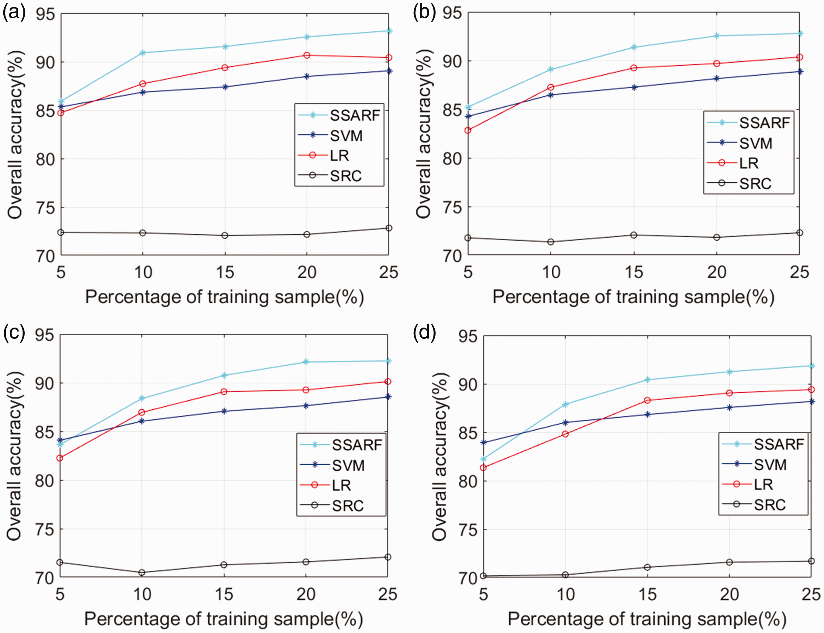
Average overall accuracy with different percentages of training samples: (a) OC 1, (b) OC 2, (c) OC 3, and (d) OC 4. SSARF: stacked sparse autoencoder random forest; SVM: support vector machine; LR: logistic regression; SRC: sparse representation classification.

First, we divide the signal into two categories: class 1 is the non-cavitation noise signals, while class 2 is the cavitation noise signals. Next, we choose a total of 150 samples as the simulation set in each of the operating conditions, and then 20% of the samples from each class are randomly chosen as the training set, and the remaining samples as the testing ones. The classification accuracy levels of the proposed approach and other compared methods are represented in Table 1. The SSA-mRMR-RF largely generated a better performance than SVM, LR, and SRC for the same feature set. The highest OA reached 93.18%. SSA-mRMR-RF shows a 3.85% higher OA compared to SVM. It also shows a 2.44% higher OA than the LR. In addition, it shows a 20.30% higher OA than the SRC on the average. The SSA-RF-based classification approaches turned out to be very effective for the classification of cavitation noise signals.

Table 1.

Class accuracies (%), overall accuracy (OA), and Kappa coefficient (κ) of two classifications.

	Class 1	Class 2	OA	κ
OC 1
SSA-mRMR-RF	90.33	95.23	92.78	0.8577
SVM	79.53	98.20	88.87	0.7773
LR	83.00	97.60	90.35	0.8070
SRC	55.83	88.77	72.30	0.4460
OC 2
SSA-mRMR-RF	90.87	95.50	93.18	0.8637
SVM	79.90	98.20	89.05	0.7810
LR	82.37	98.47	90.42	0.8083
SRC	57.43	88.20	72.82	0.4563
OC 3
SSA-mRMR-RF	88.78	94.94	91.86	0.8372
SVM	77.90	98.47	88.18	0.7637
LR	80.77	98.03	89.40	0.7880
SRC	55.97	87.43	71.70	0.4340
OC 4
SSA-mRMR-RF	89.27	95.20	92.23	0.8447
SVM	78.73	98.30	88.52	0.7703
LR	82.10	98.13	90.12	0.8023
SRC	57.07	87.10	72.08	0.4417

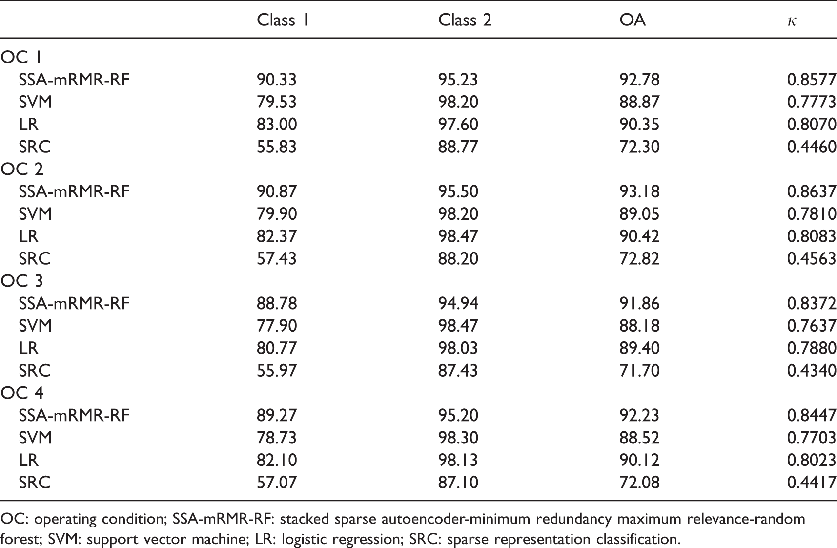
OC: operating condition; SSA-mRMR-RF: stacked sparse autoencoder-minimum redundancy maximum relevance-random forest; SVM: support vector machine; LR: logistic regression; SRC: sparse representation classification.

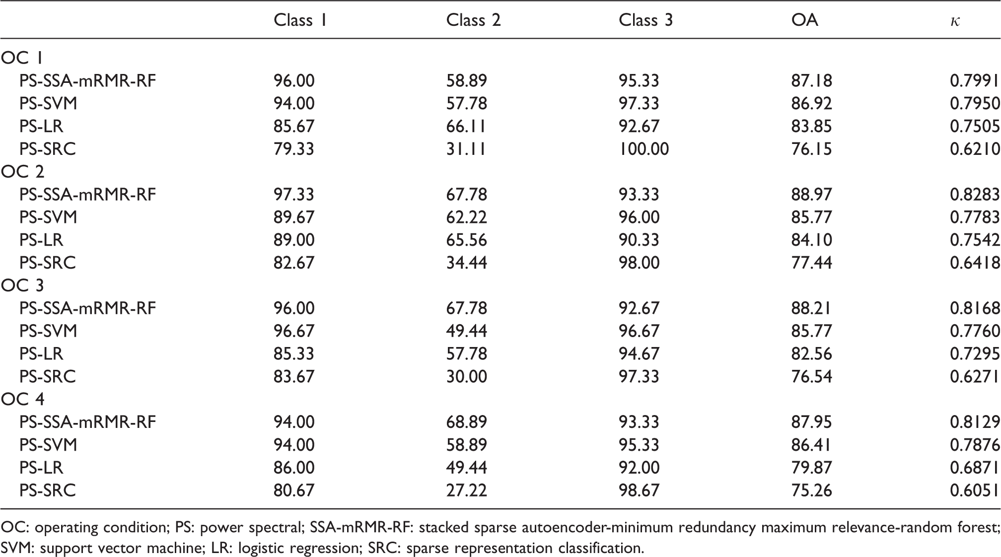
Next, we divide the signal into three categories: class 1 for the non-cavitation noise signals, class 2 for the incipient-cavitation noise signals, and class 3 for the super-cavitation noise signals. We still chose 150 samples as the simulation set in each of the operating conditions, and then 20% of the samples from each class are randomly chosen as training set, and the remaining samples as testing ones. The classification of the accuracy levels of the proposed approach and other compared methods is represented in Table 2. Although the SSA-mRMR-RF generates a better performance than the SVM, LR, and the SRC for the same feature set, the highest OA only reached 71.88%. In addition, the classification accuracy of the incipient noise signals is very low. The SSA-mRMR-RF-based classification approaches turned out to be ineffective for the classification of the incipient-cavitation noise signals.

Table 2.

Class accuracies (%), overall accuracy (OA), and Kappa coefficient (κ) of three classifications.

	Class 1	Class 2	Class 3	OA	κ
OC 1
SSA-mRMR-RF	75.13	36.28	88.03	71.13	0.5514
SVM	67.20	32.50	95.97	70.26	0.5343
LR	65.27	32.72	96.23	69.67	0.5257
SRC	48.13	44.89	42.33	45.15	0.1778
OC 2
SSA-mRMR-RF	76.63	35.44	89.00	71.88	0.5627
SVM	66.03	34.28	96.93	70.59	0.5401
LR	68.47	32.61	96.50	70.97	0.5452
SRC	46.83	44.17	44.73	45.41	0.1808
OC 3
SSA-mRMR-RF	67.90	33.33	96.93	71.09	0.5474
SVM	69.60	37.94	88.10	69.41	0.5267
LR	73.20	35.17	87.90	70.08	0.5350
SRC	46.73	45.67	44.67	45.69	0.1854
OC 4
SSA-mRMR-RF	73.73	36.72	87.20	70.37	0.5400
SVM	67.30	29.56	97.17	69.98	0.5300
LR	67.73	31.39	95.83	70.15	0.5321
SRC	46.87	42.67	46.03	45.58	0.1826

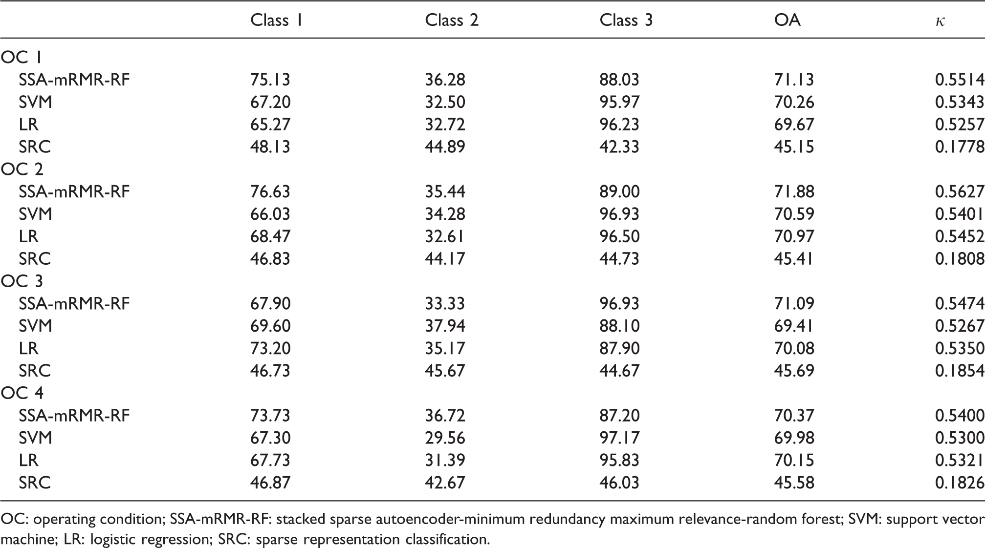
OC: operating condition; SSA-mRMR-RF: stacked sparse autoencoder-minimum redundancy maximum relevance-random forest; SVM: support vector machine; LR: logistic regression; SRC: sparse representation classification.

The power spectral (PS) density indicates the change of the signal power with frequency. The PS density of the four different operating conditions is shown in Figure 5. After obtaining the PS density curves of the different values of σ, we have found that some of the curves nearly coincide. This shows that the similar state of cavitation has similar curves, and this can distinguish the different states of cavitation. The same color is used in Figure 5 to stamp the curve where the cavitation conditions are similar. Then we can use the characteristic of the PS density to judge whether the incipient cavitation occurs.

Figure 5.

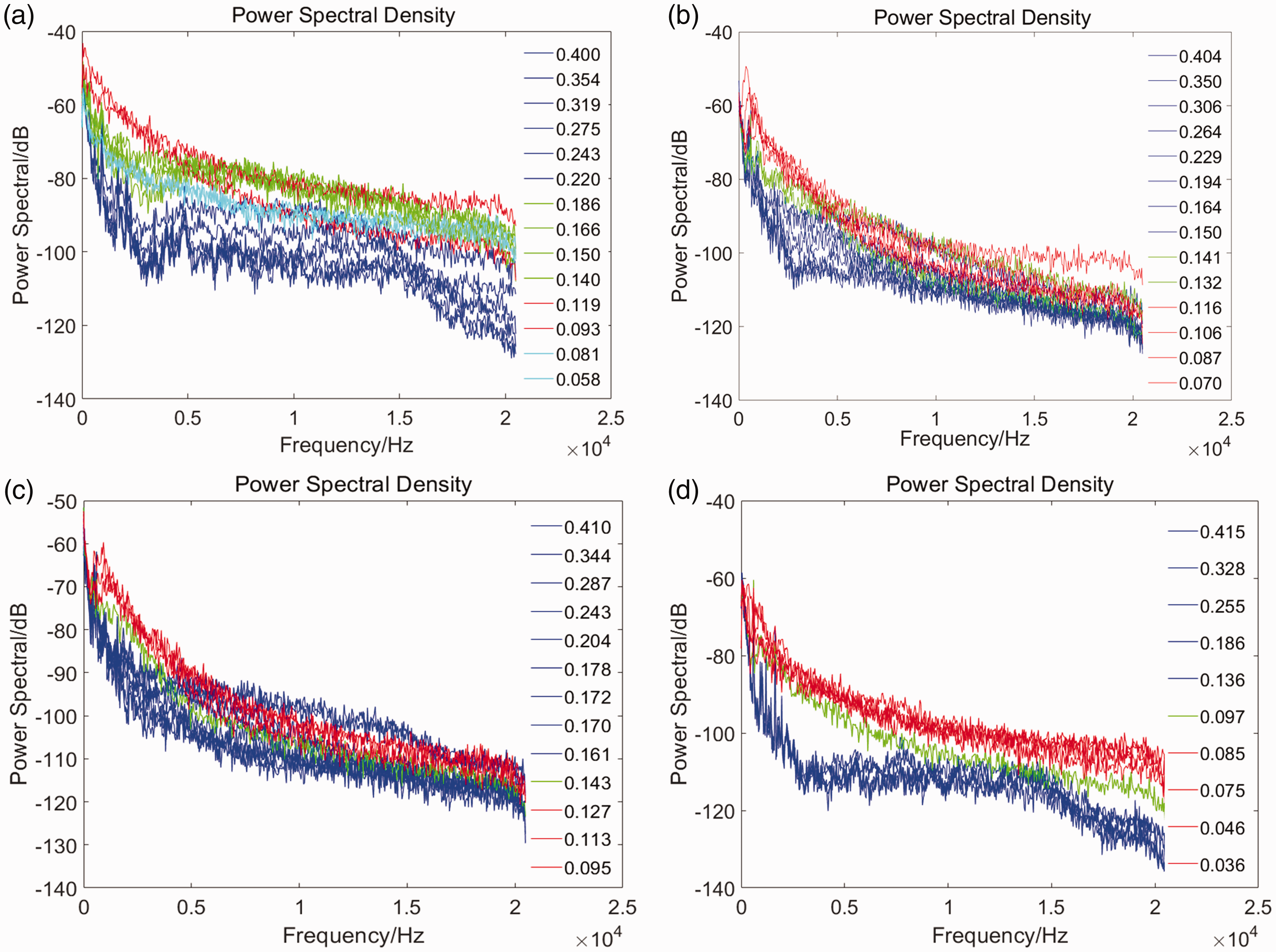
Power spectral density of the noise signals: (a) OC 1, (b) OC 2, (c) OC 3, and (d) OC 4.

The wavelet time–frequency analysis of the noise signals is shown in Figure 6. We chose the Morlet wavelet basis here. The range of the abscissa in Figure 6 is 0–10 s. The range of ordinate in Figure 6 is 0–20 kHz. Each column in the figure has the same operating condition, and each row in the figure has the same cavitation state. The detailed value of $\sigma$ for each subgraph in Figure 6 is shown in the corresponding Table 3.

Figure 6.

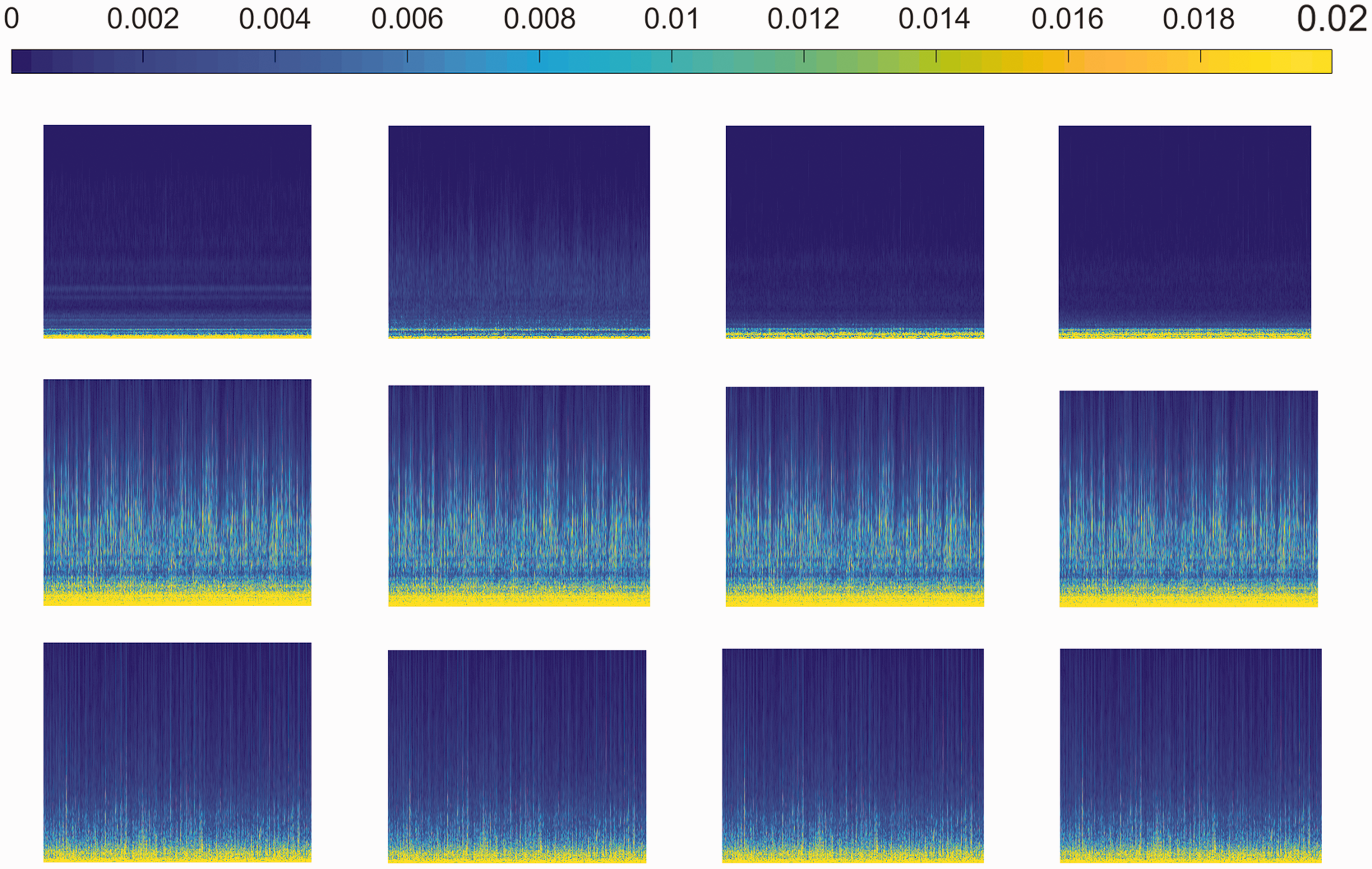
The wavelet time–frequency analysis of the noise signals for hydrophone.

Table 3.

The detailed value of $\sigma$ for each subgraph.

	OC 1	OC 2	OC 3	OC 4
None cavitation	0.400	0.410	0.415	0.412
Incipient cavitation	0.150	0.170	0.085	0.096
Super cavitation	0.119	0.143	0.075	0.066

OC: operating condition.

From Figure 6, it can be noted that in the absence of cavitation, the frequency value of the four operating conditions are all below the 0.4 kHz during the entire period, and it is the typical frequency of the hydraulic turbine ambient noise when there is no cavitation. The state of incipient cavitation has the frequency value which ranges from 0 kHz to 20 kHz. When it reached super cavitation, lots of bubbles appear and collapse, and the frequency energy becomes stronger. The time for bubbles to collapse is very short, usually in nanoseconds only, and can be seen as a narrow peak sound pressure pulse. When the cavitation is strong, the characteristic frequency spectrum of the cavitation shifted to low frequency and the value of the peak will increase. This explains the phenomenon of incipient cavitation reasonably. Above all, the wavelet time–frequency analysis of the noise signals can distinguish the different operating conditions, and it can also discriminate between the occurrence of incipient cavitation and the other states of cavitation.

In summary, we strongly suggest the frequency characteristics of the cavitation noise signal as a basis for classification, and we also propose the PS-SSA-mRMR-RF and the fast Fourier transform (FFT)-SSA-mRMR-RF models to be used. The classification of the accuracy levels of the proposed approach and other compared methods based on PS density is well represented in Table 4. The accuracy of non-cavitation noise signals and super-cavitation signals are high as shown in Table 4. The non-cavitation noise signals and the super-cavitation signals are more similar than the incipient-cavitation signals. This shows that the characteristics of the non-cavitation noise signals and the super-cavitation signals are more uniform or similar; this also shows that the accuracy is high. But the OA of our method is higher than others, and we have just divided signals into three categories. There are also two kinds of signals with high classification accuracy, and the rest of the signals are naturally separated. The classification accuracy levels of the proposed approach and the other compared methods based on the FFT are represented in Table 5. The SSA-mRMR-RF still largely generates a better performance than the SVM, LR, and the SRC for the same feature set. The highest OA reached 88.97% in Table 4 and 96.05% in Table 5. The SSA-mRMR-RF based on frequency characteristics classification approaches turned out to be very effective for the accurate classification of cavitation noise signal.

Table 4.

Class accuracies (%), overall accuracy (OA), and Kappa coefficient (κ) of three classifications based on power spectral.

	Class 1	Class 2	Class 3	OA	κ
OC 1
PS-SSA-mRMR-RF	96.00	58.89	95.33	87.18	0.7991
PS-SVM	94.00	57.78	97.33	86.92	0.7950
PS-LR	85.67	66.11	92.67	83.85	0.7505
PS-SRC	79.33	31.11	100.00	76.15	0.6210
OC 2
PS-SSA-mRMR-RF	97.33	67.78	93.33	88.97	0.8283
PS-SVM	89.67	62.22	96.00	85.77	0.7783
PS-LR	89.00	65.56	90.33	84.10	0.7542
PS-SRC	82.67	34.44	98.00	77.44	0.6418
OC 3
PS-SSA-mRMR-RF	96.00	67.78	92.67	88.21	0.8168
PS-SVM	96.67	49.44	96.67	85.77	0.7760
PS-LR	85.33	57.78	94.67	82.56	0.7295
PS-SRC	83.67	30.00	97.33	76.54	0.6271
OC 4
PS-SSA-mRMR-RF	94.00	68.89	93.33	87.95	0.8129
PS-SVM	94.00	58.89	95.33	86.41	0.7876
PS-LR	86.00	49.44	92.00	79.87	0.6871
PS-SRC	80.67	27.22	98.67	75.26	0.6051

OC: operating condition; PS: power spectral; SSA-mRMR-RF: stacked sparse autoencoder-minimum redundancy maximum relevance-random forest; SVM: support vector machine; LR: logistic regression; SRC: sparse representation classification.

Table 5.

Class accuracies (%), overall accuracy (OA), and Kappa coefficient (κ) of three classifications based on FFT.

	Class 1	Class 2	Class 3	OA	κ
OC 1
FFT-SSA-RF	88.40	88.17	98.07	95.91	0.9370
FFT-SVM	99.30	81.39	97.13	94.33	0.9123
FFT-LR	98.40	81.89	96.60	93.90	0.9057
FFT-SRC	69.10	36.78	94.97	71.59	0.5508
OC 2
FFT-SSA-RF	99.33	87.61	97.83	96.05	0.9391
FFT-SVM	99.07	83.22	95.93	94.21	0.9106
FFT-LR	98.60	82.44	97.60	94.49	0.9148
FFT-SRC	69.80	37.44	94.90	71.99	0.5568
OC 3
FFT-SSA-RF	98.60	86.06	98.10	95.51	0.9307
FFT-SVM	98.27	82.39	96.60	93.96	0.9068
FFT-LR	98.33	78.78	97.67	93.56	0.9003
FFT-SRC	71.77	38.67	95.17	73.13	0.5749
OC 4
FFT-SSA-RF	98.40	88.22	98.27	96.00	0.9383
FFT-SVM	98.40	83.00	96.80	94.23	0.9109
FFT-LR	99.07	79.22	96.93	93.67	0.9019
FFT-SRC	69.57	36.44	94.23	71.41	0.5479

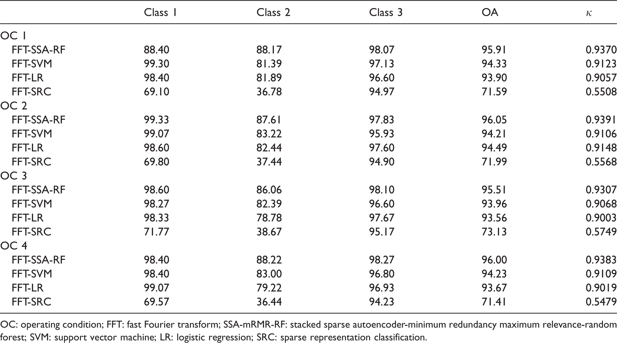
OC: operating condition; FFT: fast Fourier transform; SSA-mRMR-RF: stacked sparse autoencoder-minimum redundancy maximum relevance-random forest; SVM: support vector machine; LR: logistic regression; SRC: sparse representation classification.

Conclusion

In this paper, a method based on the SSA-mRMR-RF has been proposed to extract multiple features for the classification of the cavitation noise signal data. First of all, the SSA-mRMR-RF largely generates a better performance than the SVM, LR, and SRC for the same feature set. The highest overall accuracy reached 93.18%. SSA-mRMR-RF generated a 3.85% higher overall accuracy than SVM. It also shows a 2.44% higher overall accuracy than the LR. In addition, it shows a 20.30% higher overall accuracy than the SRC on the average. When we divide the signal into three categories, the highest overall accuracy decreased to 71.88%, and this showed that the classification accuracy of the incipient noise signals is very low. Then, we suggest the frequency characteristics of the cavitation noise signal as a basis for classification of cavitation. We also propose the use of the PS-SSA-mRMR-RF and FFT-SSA-mRMR-RF models. The highest overall accuracy rebound went back to 88.97% based on the power spectrum, and 96.05% based on the FFT. Above all, the SSA-mRMR-RF based on frequency characteristics classification approaches turned out to be very effective for the accurate classification of cavitation noise signal.

This method also has limitations and shortcomings, for example, it must satisfy a certain number of training samples so that the classification accuracy can meet the requirements. However, the methods proposed in this paper were proven to improve the identification rate of cavitation occurrence and guide the monitoring of the hydro turbine cavitation occurrence in hydroelectric power plants. It will also help prevent the damage on turbine blades caused by cavitation and improve the power generation efficiency to a certain extent. These findings show that this paper indeed has significant and practical benefits for the hydroelectric power stations that we currently have.