
Abstract
Grinding wheel condition is considered as the key factor affecting grinding performance, and therefore, accurate monitoring of wheel wear is necessary to prevent the deterioration of part quality. An intelligent wheel wear monitoring system is introduced in this article to realize processing of grinding signal, extraction of signal features, selection of optimal feature subset, and prediction of wheel wear. Physical information generated during the grinding of C-250 maraging steel is collected by a dynamometer, accelerometer, and acoustic emission sensor, and a large quantity of features in time domain and frequency domain are extracted from the processed grinding signals. To reduce feature redundancy and increase relevancy of feature to wheel wear, a two-stage feature selection approach combining filter and wrapper framework is proposed. The filter preselects individual features by minimum Redundancy Maximum Relevance method, while the wrapper evaluates different feature subsets by the model performance. A deep learning network structure named Long Short-Term Memory network is adopted to develop the wheel wear monitoring model and is compared with a conventional machine learning algorithm, Random Forest. The results have shown that the two-stage feature selection method is able to provide the globally optimal feature subset for the model. Long Short-Term Memory model achieves an R2 of 0.994 and a root-mean-square error of 0.240 with four features, while Random Forest model obtains an R2 of 0.980 and a root-mean-square error of 0.463 with seven features, which indicates that Long Short-Term Memory model is capable of predicting wheel wear more accurately even with less features.
Keywords
Introduction
C-250 maraging steel is widely used in the manufacturing of automobile, medical apparatus, and aerospace equipment because of their ultra-high strength and excellent malleability. However, maraging steels are a class of difficult-to-machine materials and require grinding as a final machining process to achieve good surface finish and low residual stress. In grinding, an abrasive wheel rotates at a high speed to remove material from the surface of a manufactured part. Wheel wear inevitably occurs during the grinding process, leading to a dull grinding wheel, and could result in a rough surface finish, surface thermal damage, or chatter marks on the parts.1–6 Considering the high demands in the machining of C-250 maraging steel, the grinding wheel must be inspected periodically to prevent deterioration of the part quality. Dressing or truing should be applied to achieve favorable abrasiveness of the wheel when wear is severe. Thus, monitoring of wheel wear in grinding process is essential to detect these issues in advance and avoid manufacturing defective parts.
Various wheel wear monitoring techniques, which can be divided into direct and indirect approaches, have been presented in the literature. The utilization of charge-coupled device (CCD) cameras and microscopes7–9 provides a visualized inspection of wheel wear directly, whereas these instruments are not feasible to be implemented online due to the cost of capital and time. Thus, some indirect methods are adopted to estimate or predict wheel wear by means of collecting and studying diverse physical phenomena during grinding process with various sensors. Several signal features, such as mean values of the power 10 and force 11 signal, the mean value, root mean square (RMS), and amplitude of the frequency spectrum11,12 in acceleration signal, are commonly selected to detect the wheel condition. In addition, features in acoustic emission (AE) signal, for example, RMS,12–14 amplitude, 15 and power spectral density (PSD)10,13,15, have been proved to be the effective tools to monitor wheel wear.
With the widespread use of machine learning in grinding process in the past decade, physical-based models that require profound understandings of comprehensive grinding mechanisms9,16,17 have been gradually replaced by intelligent data-driven monitoring systems due to the complex underlying physics and a lack of generalization modeling approaches. Liao et al. 10 introduced a clustering method that involves extracting features from AE signals based on discrete wavelet decomposition to predict wheel condition. The results indicated that the proposed methodology could achieve clustering accuracies of 97%, 86.7%, and 76.7% for the high material removal rate condition, low material removal rate condition, and combined grinding conditions, respectively. Yang and Yu 14 proposed a grinding wheel wear monitoring system based on discrete wavelet decomposition and support vector machine classification. A classification accuracy of 99.39% with a cut depth of 10 µm and a classification accuracy of 100% with a cut depth of 20 µm could be obtained by the proposed system. A virtual sensor based on an artificial neural network for wheel wear monitoring was presented by Arriandiaga et al. 18 and achieved an accuracy of approximately 80% under known grinding conditions. To build an intelligent wheel wear monitoring system, Nakai et al. 19 composed four types of neural networks: multilayer perceptron (MLP), a radial basis function neural network (RBFNN), a generalized regression neural network (GRNN), and an adaptive neuro-fuzzy inference system (ANFIS). The best result was a success rate of 95.8% for the high material removal rate condition using the RBFNN and a 96.2% success rate for the low material removal rate condition using MLP.
Deep learning, as an extension of machine learning, has been adopted to deal with image classification, speech recognition, and text processing tasks in these years. Four prevalent architectures of deep learning algorithms, namely, Convolutional Neural Network (CNN), Recurrent Neural Network (RNN), Restricted Boltzmann Machine (RBM), and Autoencoder, have shown overwhelming advantages in model performance over conventional machining learning algorithms. 20 The study of deep learning in manufacturing currently focuses on fault diagnosis,21–24 whereas there is less research in tool condition monitoring. Zhao et al. 25 proposed a deep neural network structure named Convolutional Bi-directional Long Short-Term Memory (CBLSTM) networks to predict tool wear in dry milling. The CBLSTM was compared with RNN and its variant models, and showed least mean absolute error and root-mean-square error (RMSE) among all the models.
The aforementioned review of literature demonstrates that the monitoring of wheel wear has been more scientific with the aids of signal processing techniques and machining learning approaches. However, features related to the wheel wear are typically chosen empirically in most research and the accuracy of monitoring model could be further improved. In order to address these two issues, this study focuses on the establishment of an intelligent wheel wear monitoring system. The system collects force, acceleration, and AE signals during the grinding of C-250 maraging steel and extracts numerous time-domain and frequency-domain features from processed signals. A two-stage feature selection approach is proposed to preselect features with low redundancy and high relevancy to the wheel wear at first and then choose the optimal feature subset for the monitoring model in order to achieve best prediction accuracy. Considering that the grinding signals can be expressed in a time-series form, a sequential deep learning framework, Long Short-Term Memory (LSTM) network, is employed to develop the monitoring model and the results are compared with those of a model based on a conventional machining learning algorithm.
Methodology
Signal processing
The information from the original signals is limited; therefore, diverse signal processing techniques are utilized to capture more characteristics of the signals for further feature extraction.
Wavelet packet decomposition
Wavelet packet decomposition (WPD) is a generalized form of wavelet decomposition that offers a full range of frequency band for the signal analysis. The original signal passes through a low-pass filter and a high-pass filter, and is split into an approximation coefficient and a detail coefficient at each node.26,27 The basis of WPD is wavelet, which can be calculated from
where aw is the scaling parameter and bw is the translation parameter.
The wavelet packet coefficient cw, relating to the original signal x(t), is given by
In order to calculate the wavelet packet coefficient with computer, dyadic discretization is the most common method to transform signals from continuous domain to discrete domain by replacing aw and bw with 2n and k2n, where n is the decomposition level.
Ensemble empirical mode decomposition
Huang et al. 28 introduced empirical mode decomposition (EMD) as an adaptive time-frequency analysis method representing nonlinear signals as sums of simpler components with amplitude and frequency modulated parameters. The EMD decomposes signals into several intrinsic mode functions (IMFs), and each IMF component contains the local characteristic signal of the original signal at different time-frequency scales, as expressed by
where ci(t) is the ith IMF and rn(t) is the residual function after n IMFs are extracted.
The EMD method automatically generates a collection of IMFs by satisfying two conditions:
In a complete dataset, the number of extrema and the number of zero-crossings must either be equal or differ not more than by one.
At any point, the mean value of the envelope defined by the local maxima and the envelope defined by the local minima is zero.
Although the EMD is widely applied to decompose nonstationary signals, it has a major drawback of mode mixing. Mode mixing is defined as a single IMF either consisting of signals of widely disparate scales or a signal of a similar scale residing in different IMF components. 29 To overcome this issue, Wu and Huang 30 proposed the ensemble empirical mode decomposition (EEMD) by adding white noise to the original signal. Then, the EEMD is developed as follows:
Decompose the data with added white noise into IMFs using EMD;
Repeat Step 1 with different white noise each time;
Acquire the ensemble means of corresponding IMFs of the decompositions.
Feature extraction
In this step, various features in time domain and frequency domain will be extracted from processed signals in order to provide a large amount of preliminary features for feature selection. For all the original signals and their decomposed signals, the time-domain features include the RMS, mean, standard deviation (SD), skewness, kurtosis, peak-to-peak value, crest factor, and entropy. The frequency-domain features, which are calculated with PSD estimated by the Welch method, 31 include mean, SD, skewness, kurtosis, peak value, peak frequency, crest factor, and frequency centroid of the PSD. The definitions of all the features are listed in Table 1.
Features in time domain and frequency domain.
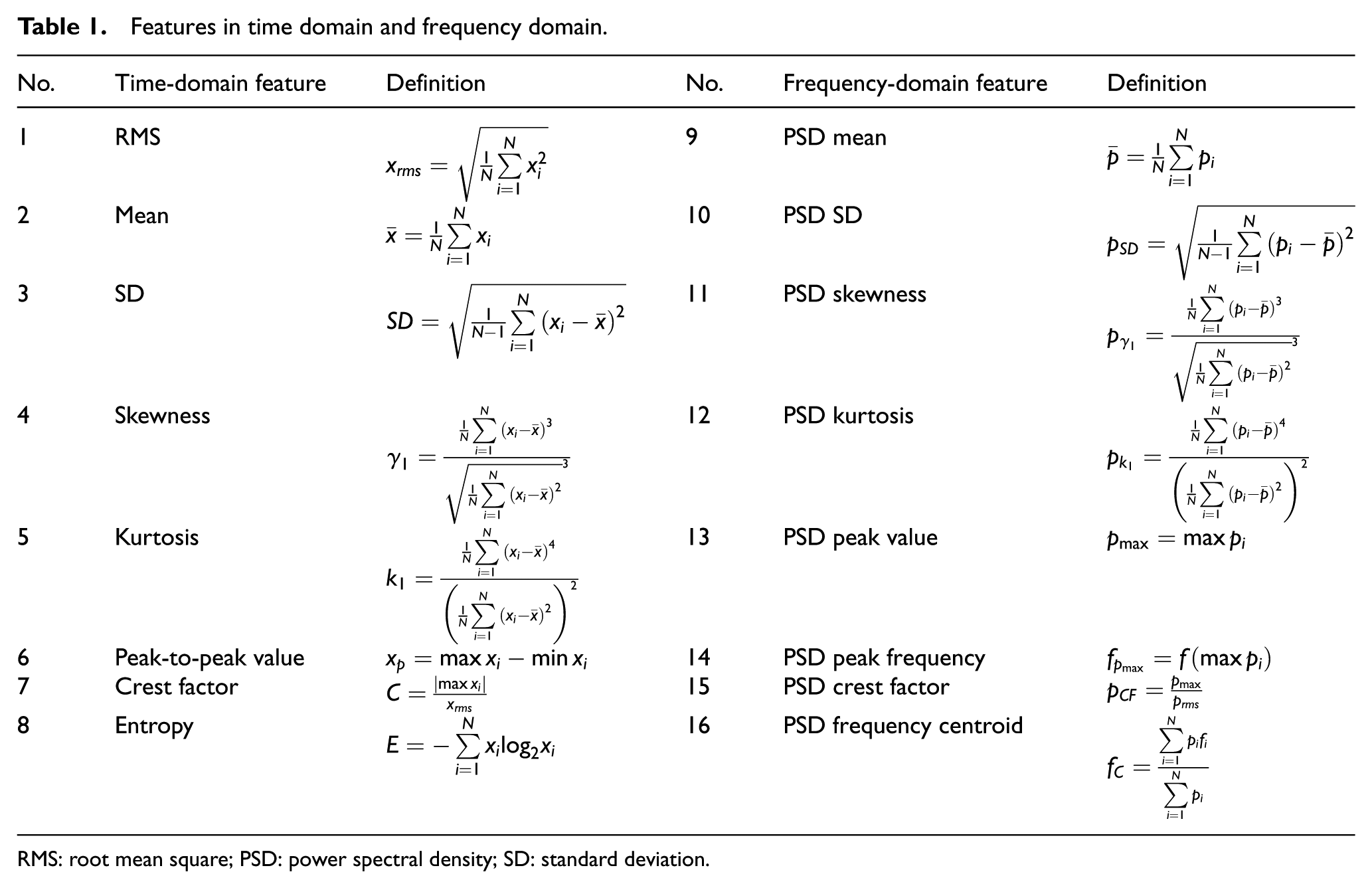
RMS: root mean square; PSD: power spectral density; SD: standard deviation.
Feature selection
The primary task in feature selection is to choose a subset of features that can provide sufficient information of wheel wear among thousands of features extracted from the original signals. The selection methods are generally classified as filter, wrapper, and embedded method. 32 Filter method is adopted to rank features based on a specific criterion, which is independent of the chosen model. Wrapper method evaluates features according to the performance of the model, and the selected features are capable of giving the best predictive power. Embedded method incorporates feature selection as part of the training process in building a specific model.
In this study, a filter method, minimum Redundancy Maximum Relevance 33 (mRMR), was applied to remove the features irrelevant to the wheel wear and reduce the redundancy among features. Each feature is scored based both on its relevance to the targets and its redundancy to other features. Mutual information (MI) is the criterion for measuring relevance and redundancy of the feature, which is defined as follows
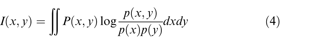
where x and y are variables, p(x, y) is the joint probabilistic density, and p(x) and p(y) are the marginal probabilistic densities.
The relevance D of the feature xi

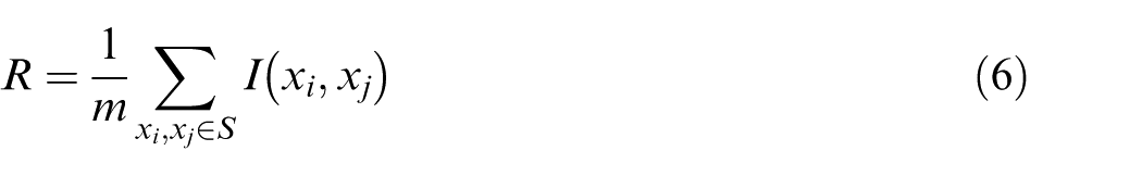
The redundancy R of the feature xi with other features xj (i≠j) in the feature subset S can be calculated by
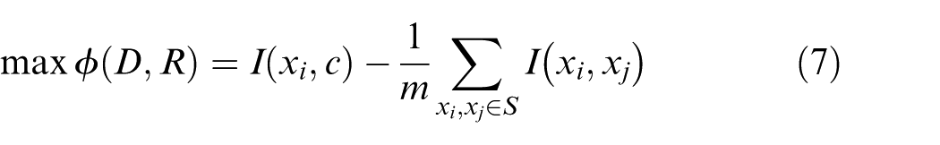
The mRMR ranks features by simultaneously maximizing the relevance D and minimizing the redundancy R. An operator φ, which can be considered as the score of each feature, is defined to combine D and R in the following form
The filter method can select features rapidly based on the intrinsic properties of the data. However, the chosen features might not be the best ones for the prediction model because the method does not interact with the model during the selection. To address this drawback, the filter method is used as a preselection and is combined with the wrapper method in order to achieve both fast selection of features and high accuracy of prediction model.34–36 This is because the dimension of features decreases remarkably using mRMR so that the exhaustive search can be applied in the wrapper method to find the globally optimal feature subset by considering the model performance. Consequently, a two-stage feature selection approach combining mRMR and machine learning algorithm is proposed in this study to select the best subset of features and establish an accurate prediction model of wheel wear.
Machine learning algorithms
Random Forest
Random Forest (RF) builds an ensemble of decision trees and outputs the aggregative results.37,38 In RF, two-thirds of the total data are used to construct trees, and the remaining one-third of the data, called “out-of-bag” (OOB) data, are used to adjust the performance of the trees. The process of regression prediction using RF is as follows:
Provided that the size of training data is N, the bootstrap aggregating process generates k (k < N) samples as the new training data by repeatedly selecting random samples with a replacement process, and constructs k decision trees.
If the D is the dimension of features in the bootstrap samples, d
The leaf node grows naturally without pruning, in order to reach maximum split depth.
The mean of the aggregating predictions from all the trees is the final result of RF.
By combining each decision tree as an individual learning model linearly, the total variance of RF is less than that of any single tree. During the reduction of error, RF tends to choose models with better self-learning ability and smaller prediction deviation so that it is capable of diminishing the noise in the predicted variable more effectively compared with artificial neural network and support vector regression. 39
LSTM network
The signals collected continuously during grinding process are in nature time series, which can represent the transformation process from a new wheel to a worn wheel. Therefore, RNN, as a prevalent architecture to handle sequential data in deep learning, is suitable to be applied in the monitoring of wheel wear. The architecture of RNN is shown in Figure 1, where the subscript indicates time step for each recurrent neuron. Unlike the neuron in the basic neural network, the output from a previous recurrent neuron Lt–1 is connected to the next recurrent neuron Lt, and the current system state ht can be characterized as a function of current data xt.
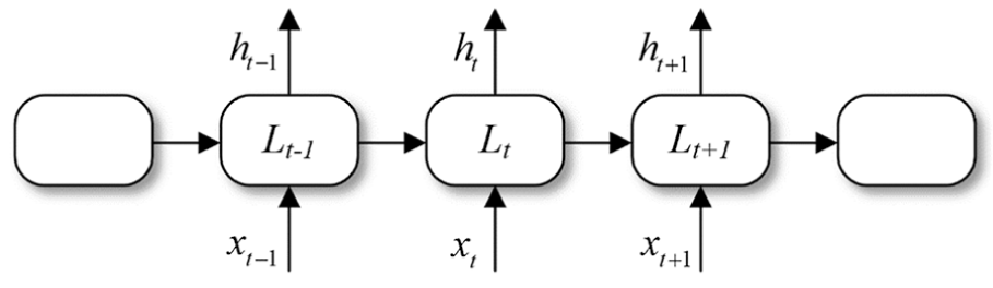
Architecture of Recurrent Neural Network.
LSTM network is a variant of RNN and addresses the problem of gradient exploding in RNN by using sigmoid or tanh function as activation function. 40 Besides, forget gates are introduced in LSTM network to avoid gradient vanishing during backpropagation in RNN and allow the model to capture long-term dependencies. These forget gates, together with input gates and output gates, enable each cell state to store or remove information adaptively.
A typical LSTM cell is illustrated in Figure 2. At each time step t, the cell receives the long-term state Ct–1, short-term state ht–1 at previous time step t–1, and current data xt. The forget gate ft controls the information removal from the previous cell, as given below

where σ is the sigmoid function; Uf and Vf are the weights of xt and ht–1 for the forget gates, respectively; and bf is the bias of the forget gate.
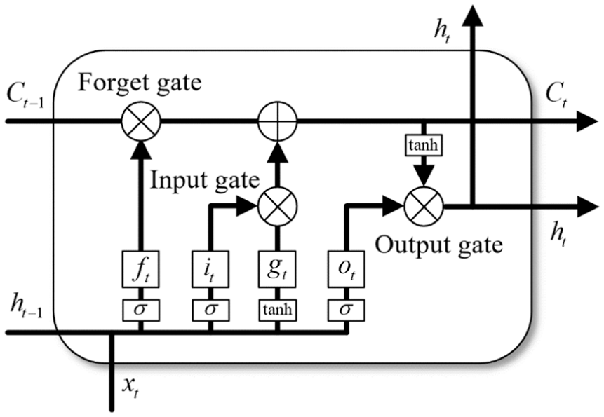
Structure of an LSTM cell.
The input gate processes xt and ht–1 in the same fashion, while a tanh activation function φ is used to create a vector of new candidate values, gt, that could be updated to the state


Then the current long-term state Ct is the combination of Ct–1, ft, it, and gt

where ⊙ denotes the element-wise product.
The short-term state in the current cell ht consists of Ct and output gate ot
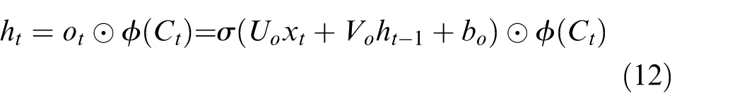
It should be noted that weights U, V, and biases b for all three gates are shared by all time steps and updated during training.
Similar to the conventional feed-forward neural networks, the weights and biases are adjusted by minimizing the loss of an objective function during the training of LSTM network. The mean squared error (MSE) is the loss function for regression problems
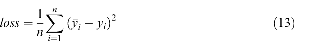
where
Intelligent monitoring system of grinding wheel wear
The proposed intelligent monitoring system of grinding wheel wear consists of signal acquisition, signal processing, feature extraction, feature selection, and development of monitoring model, as demonstrated in Figure 3. WPD and EEMD are applied to the signals collected in the grinding at first. Then features in time domain and frequency domain are extracted from processed signals. The mRMR method preselects features that have most relevance to the wheel wear and least redundancy among themselves. Feature subsets are generated by the preselected features and are used to train the monitoring model based on RF or LSTM. The best predicted values of wheel wear can be obtained by exhaustive search, and corresponding feature subset is selected as the optimal one for the monitoring of wheel wear.
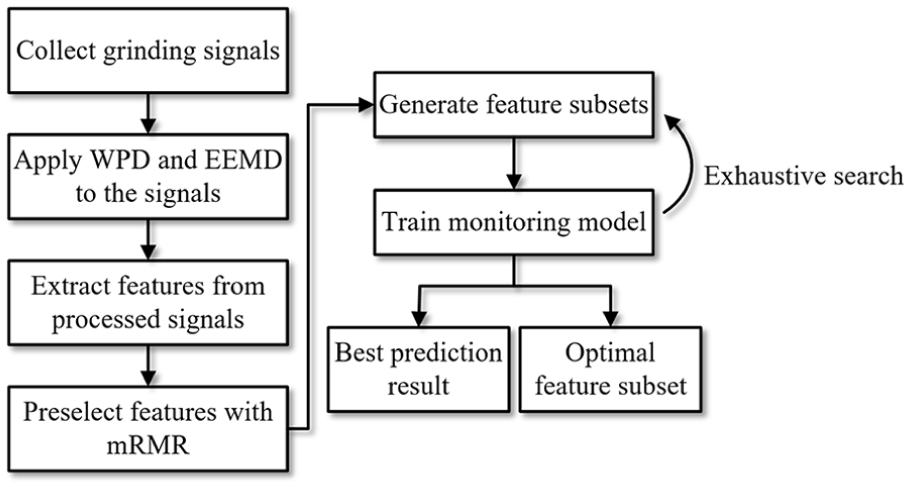
Flowchart of intelligent wheel wear monitoring system.
Experimental setup
Design of wheel wear experiment
The experiment was performed on a DMG 635V machining center. An electroplated cubic boron nitride (CBN) grinding wheel with a diameter of 12 mm and a width of 10 mm was used, and the wheel had an average grain size of 120 µm. The workpiece material was C-250 maraging steel and each specimen had a cubic dimension of 15 mm × 20 mm × 2 mm. Grinding parameters are as follows: grinding wheel velocity, vs = 5.03 m/s; workpiece speed, vw = 5.3 mm/s; depth of cut, ap = 4 µm; and specific material removal rate, Q′= 0.021 mm3/mm·s.
A schematic diagram of the experimental setup is shown in Figure 4. A multicomponent dynamometer, Kistler 9256C, mounted under the fixture of workpiece was used to measure tangential and normal grinding forces. A piezoelectric accelerometers with an operating frequency range of 0 to 5 kHz were used to measure tangential and normal vibrations. The dynamometer was connected to a charge amplifier Kistler 5080A, and both the force and acceleration signals were collected via Siemens LMS data acquisition system at a sampling frequency of 3200 Hz. A water-resistant AE sensor, Soundwel WG50, which has an operating frequency range of 100 to 1000 kHz, was used to detect stress wave released by the material removal during the experiment. The collection of AE signals was implemented by Soundwel SAEU2S DAQ system at a sampling frequency of 2000 kHz.
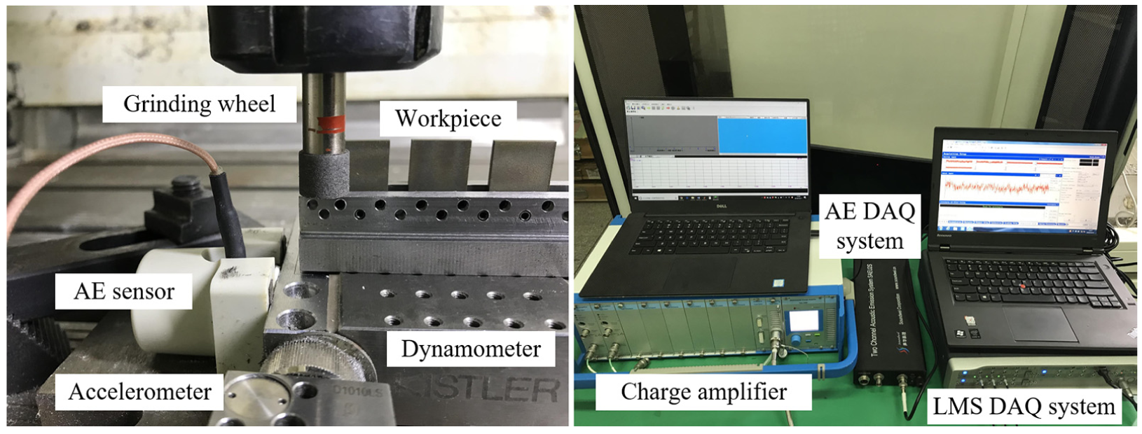
Schematic diagram of experimental setup.
Measurement of wheel wear
The measurement of the grinding wheel surface topography was carried out through a HIROX KH-7700 digital microscope. Figure 5 demonstrates sequential optical images of CBN wheel surface with increasing total material removal V during the experiment. Figure 5(a) shows the intact abrasive grains on the wheel surface before the grinding. After the first 6 mm3 of material being removed (Figure 5(b)), the grains basically preserved the original shape. Small rubbing wear flats were formed on the top of the grains when V = 12 and 18 mm3 (Figure 5(c) and (d)) and swarf adhered to the wheel surface. When V increased from 24 to 36 mm3 (Figure 5(e)–(g)), the wear flat areas of grains were gradually enlarged and the fractures were produced on the grains. The grains could be hardly distinguished from the swarf and the debris when V was more than 42 mm3 (Figure 5(h)–(j)), which manifested that the wear was severe and the wheel had lost the cutting ability to remove the material.
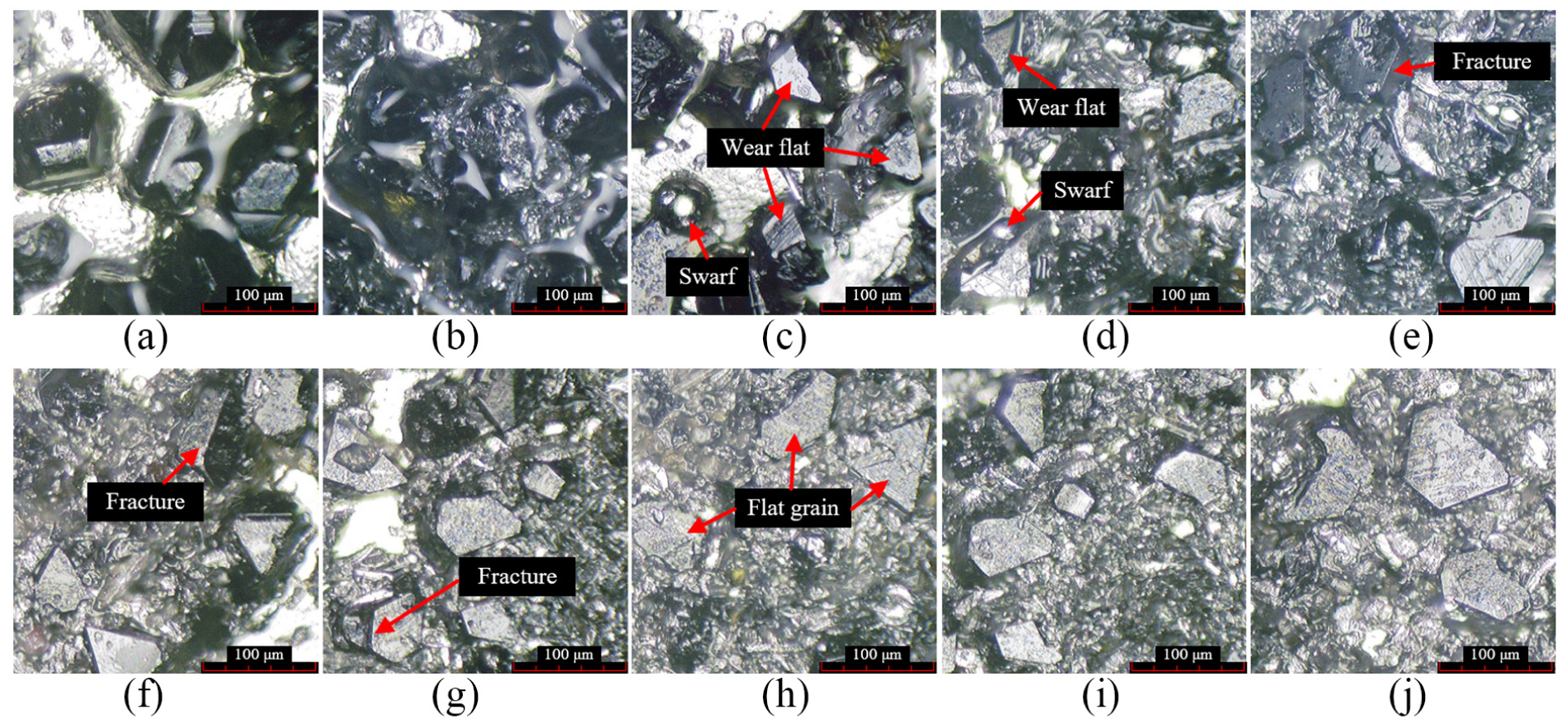
Optical microscope images of wheel surface: (a) V = 0 mm3, (b) V = 6 mm3, (c) V = 12 mm3, (d) V = 18 mm3, (e) V = 24 mm3, (f) V = 30 mm3, (g) V = 36 mm3, (h) V = 42 mm3, (i) V = 48 mm3, and (j) V = 54 mm3.
To evaluate surface topography of grinding wheel, Mainsah et al. 41 proposed 14 parameters, including amplitude, spatial, hybrid, and functional parameters. The amplitude parameter, root-mean-square deviation of the surface, Sq, is used to identify wheel wear in this study, which is expressed as
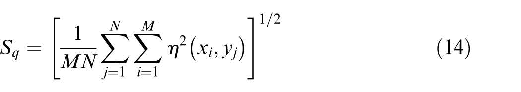
where
The three-dimensional (3D) plots of wheel surface at V = 0, 12, 24, and 48 mm3 are illustrated as the examples and the Sq of the wheel surface with various total material removals calculated from the 3D plots is shown in Figure 6. In order to extend the sample size of wheel wear for the training of wheel wear monitoring system, the discrete Sq values are fitted by a second polynomial and the coefficient of determination (R2) is up to 0.98, which allows the wheel wear being interpolated well according to the size of input samples.
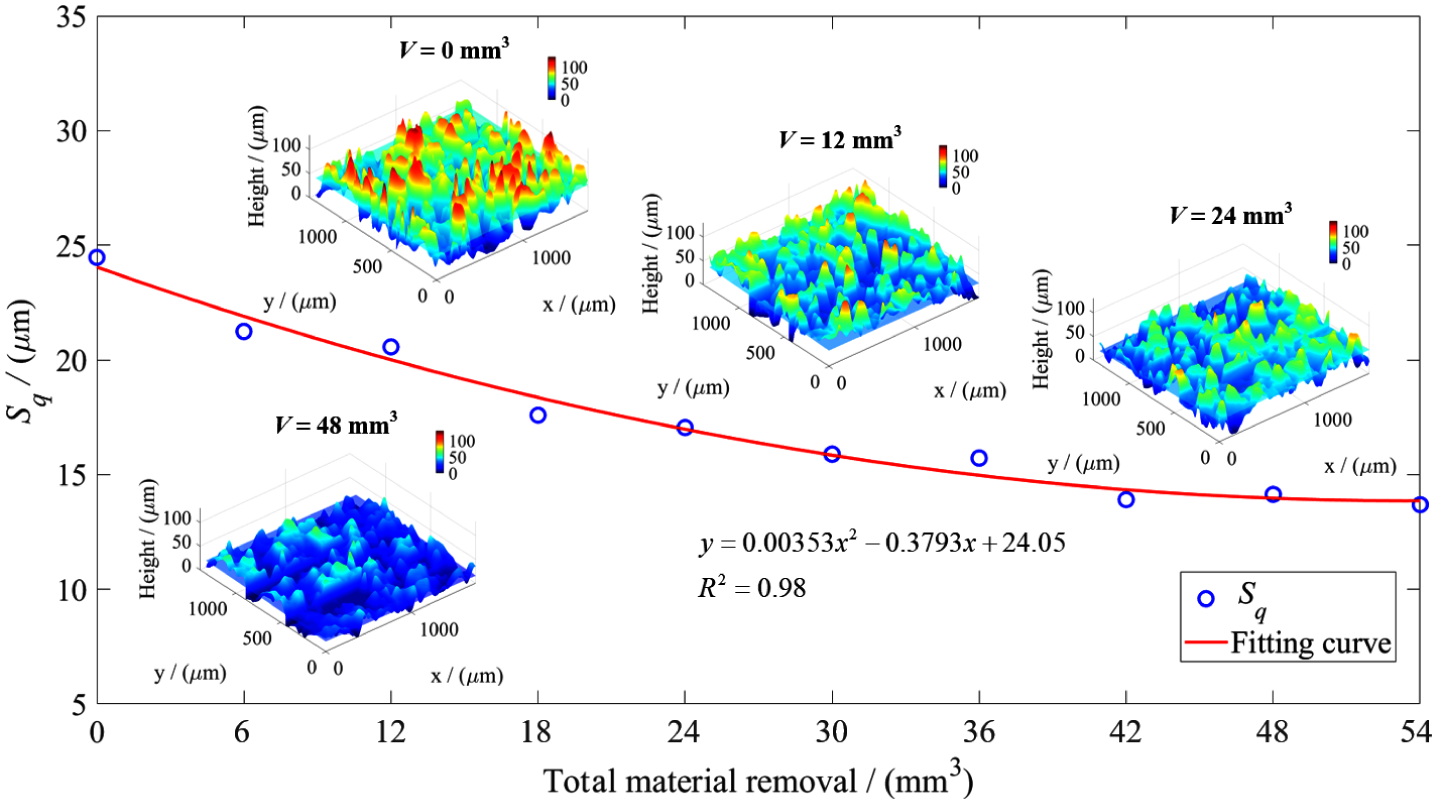
Sq and 3D plots of wheel surface with various total material removals.
Results and discussion
In order to provide sufficient preliminary features and improve the selection of the features, the force, acceleration, and AE signals were preprocessed by diverse types of filter. The original force signals were processed by low-pass filters with cutoff frequencies at 10, 20, 50, 100, 200, 300, 400, and 500 Hz, respectively. Bandpass filters with different frequency band window widths, such as 50 to 100, 50 to 150,…, 50 to 1000, 100 to 150, …, and 950 to 1000 Hz, were adopted to the force signals so as to acquire more detailed characteristics related to the grinding process. Due to the same sampling frequency being applied, the original acceleration signals underwent the identical preprocessing. An example of the original AE signal and its frequency range is shown in Figure 7, which indicates that filters can be applied within the range of 100 to 400 kHz. Thus, the frequency bands of bandpass filters for the original AE signal were 100 to 150, 100 to 200, …, 300 to 400 and 350 to 400 kHz. As a result, a total of 16,208 features were extracted, including 16 (16 types of feature in Section 2.2 Feature selection) × [8 (8 frequency bands of low-pass filters) + 190 (190 frequency bands of bandpass filters) + 30 (30 WPD nodes) + 10 (10 IMFs in EEMD)] × 2 (tangential and normal direction) = 7616 features from the force signals, 7616 features from the acceleration signals, and 16 × [21 (21 frequency bands of bandpass filters) + 30 + 10] = 976 features from the AE signal.
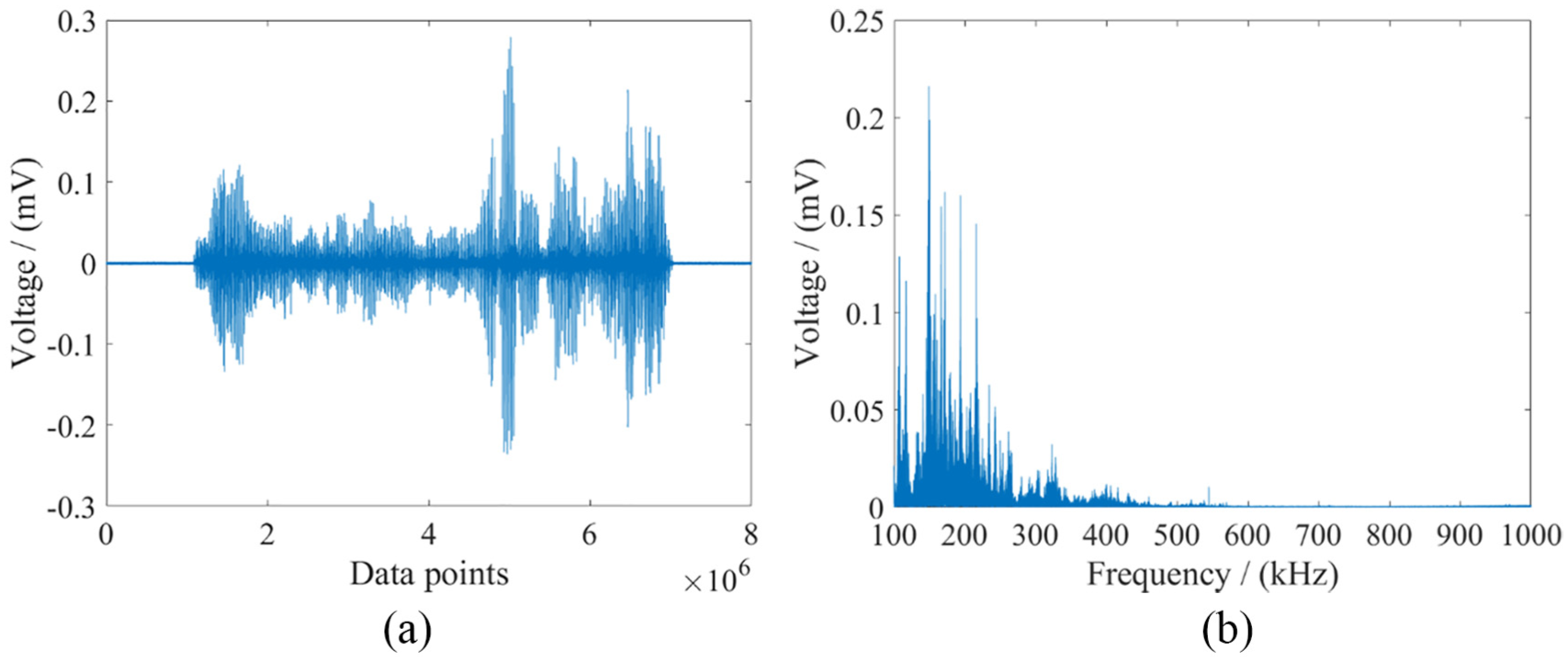
An example of (a) original AE signal and (b) its frequency range.
The mRMR method evaluated 16,208 features based on their relevance to the wheel wear and redundancy with other features. According to equation (8), the higher score a feature gets, the more important the feature would be for the monitoring of wheel wear. In order to carry out exhaustive search in the wrapper method to refine the optimal feature subset for the monitoring model, 10 features with highest mRMR scores were preselected, as listed in Table 2.
Top 10 features preselected by the mRMR method.
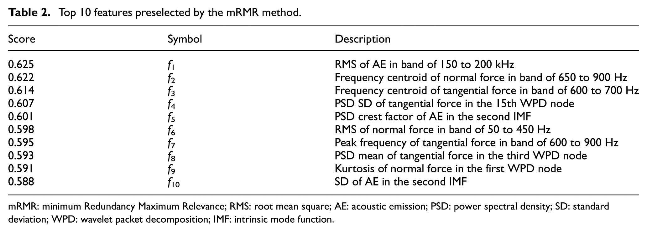
mRMR: minimum Redundancy Maximum Relevance; RMS: root mean square; AE: acoustic emission; PSD: power spectral density; SD: standard deviation; WPD: wavelet packet decomposition; IMF: intrinsic mode function.
The exhaustive search of feature subsets involved
The values of features extracted from various signals have considerable differences, and the features with larger values could be dominant in the model. Therefore, it is imperative to normalize all the selected features within the uniform scale range before the training by using equation (16)
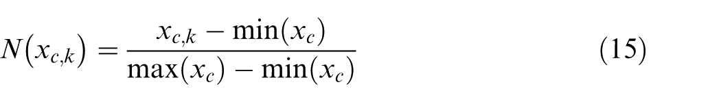
where c represents the cth feature, k represents the kth data point in the cth feature, and min(xc) and max(xc) are the minimum and the maximum values in the cth feature.
The entire grinding process took approximately 216 s in the experiment, and all the features were extracted from each second. Accordingly, a total of 216 samples were divided into training dataset and testing dataset equally. Statistical criteria—namely, the coefficient of determination (R2) and RMSE—are typically employed to assess the performance of the model. 42 R2 indicates how well the model is able to approximate the actual data points, which can be expressed as
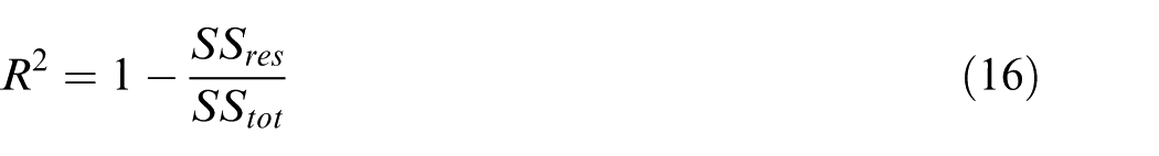
where
The number of decision trees and the number of hidden units are the primary parameters of RF and LSTM models, respectively. Thus, these parameters should be determined at first based on the best R2 and RMSE of the model using all 10 preselected features. Figure 8(a) and (b) demonstrates the relationship between the model performance and parameters in RF and LSTM models, respectively.
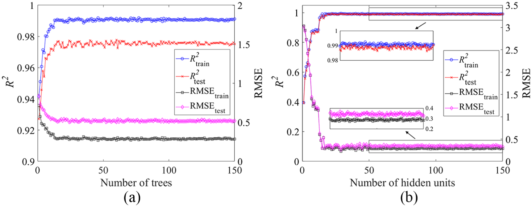
Effect of model parameters on the performance of (a) RF and (b) LSTM models.
The R2 and RMSE of RF model in both training and testing progress improve significantly in the first 15 trees. The R2 in the testing progress fluctuates from 0.97 to 0.98 when the model is trained by 15 to 60 trees, and the RMSE varies from 0.4 to 0.44 accordingly. The model performance becomes stable after 80 trees, and thus, 100 trees are selected to train RF model. Although the performance of LSTM model is poor when using a few hidden units, it improves dramatically with more hidden units. The R2 and RMSE of LSTM model in testing progress stabilize at 0.988 and 0.35, respectively, after 50 hidden nodes, and hence, 70 hidden units were considered to be sufficient to train LSTM model. In addition, the variance of model performance in training and testing progress is greater in RF model than that in LSTM model, which manifests that the RF is worse than LSTM with respect to the ability of model generalization.
According to the exhaustive search, 1023 subsets of different features in the training dataset were used individually to train the wheel wear monitoring model. Then the trained RF and LSTM models were validated by the testing dataset. The comparison of the best performance of RF and LSTM models with different number of features during testing progress is shown in Figure 9. For RF model, the R2 increases from 0.91 to 0.98 with increasing number of features and the RMSE drops from 0.94 to 0.47. The best model performance is obtained when the model is trained with a subset of seven features. The R2 and RMSE are around 0.99 and 0.3, respectively, in LSTM model, and their variations with number of features model are minor. Differing from improving with more features in RF model, the performance of LSTM model deteriorates when the number of features increases, and the best R2 and RMSE are achieved by four features. This indicates that the features preselected by the mRMR approach cannot be used directly for the development of model, and the two-stage feature selection method is able to make up the deficiency of mRMR by evaluating the effect of feature subsets on the model performance. Consequently, the feature subsets for RF and LSTM models are determined according to the best model performance and the specific feature subsets are listed in Table 3, where
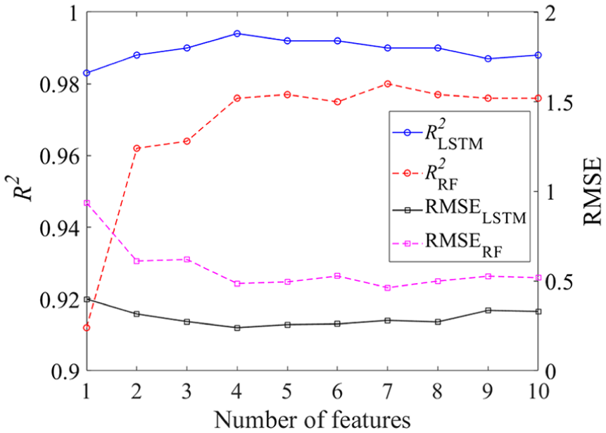
Performance of RF and LSTM models with different number of features.
Best performance of RF and LSTM models, according to optimal feature subset.
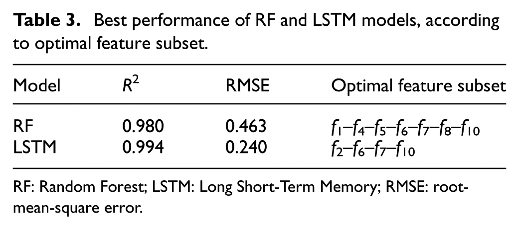
RF: Random Forest; LSTM: Long Short-Term Memory; RMSE: root-mean-square error.
Figure 10(a) and (b) illustrates the wheel wear predicted by RF and LSTM models with best predictive ability, respectively. It is obvious that the predicted wear values are more scattered in RF model, which results in the greater prediction errors. On the contrary, the wheel wear at a specific moment is predicted by the present signal features and previous wear conditions due to the characteristic of LSTM. As a result, the overall predicted wheel wear is able to follow the fitted wear curve better and no outlier is found in the LSTM model.
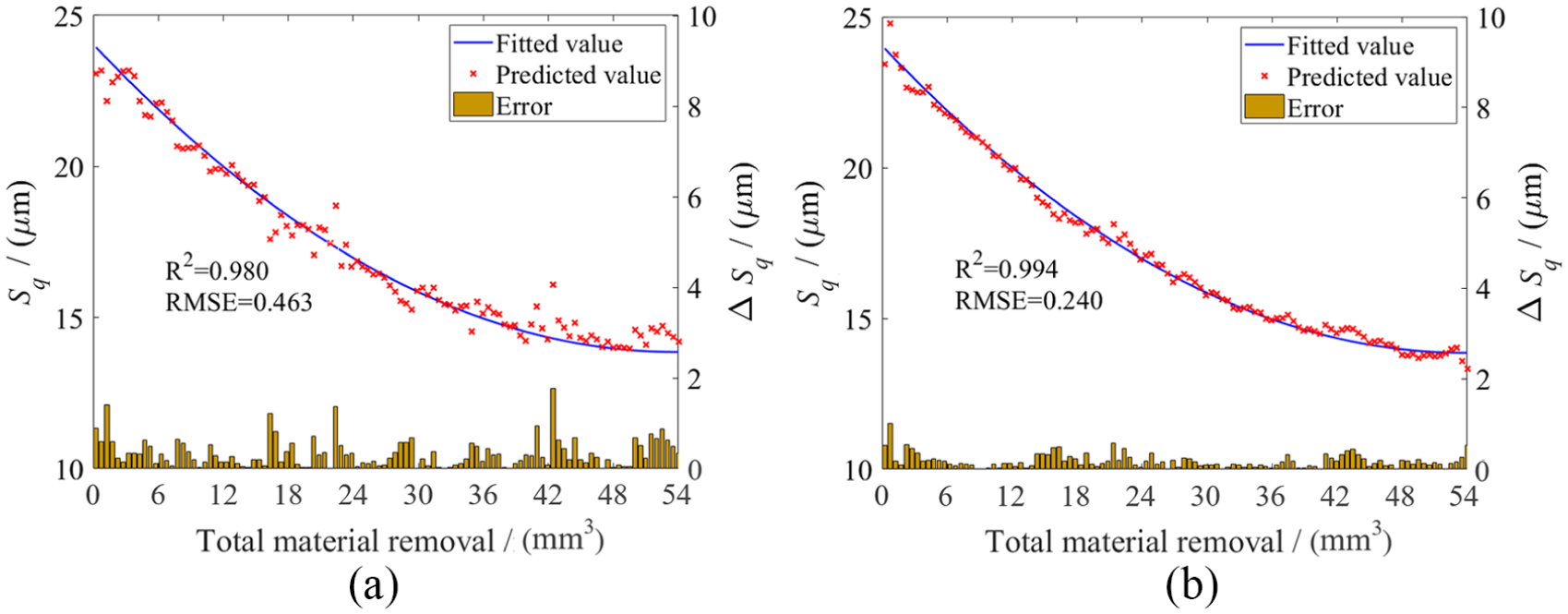
Predicted wheel wear of (a) RF and (b) LSTM models.
Conclusion
This article proposes an intelligent wheel wear monitoring system, and the system is applied to the grinding of C-250 maraging steel. The conclusions can be drawn as follows:
A two-stage feature selection method is proposed to find the globally optimal feature subset for the monitoring of wheel wear. The mRMR method removes redundant features and preselects 10 features most relevant to the wheel wear among 16,208 extracted features at first. Then, the wrapper method executes exhaustive search to refine the optimal feature subset according to the best predictive ability of the monitoring model.
A deep learning algorithm, LSTM, is employed to develop the wheel wear monitoring model, and another model based on conventional machine learning algorithm, RF, is established for comparison. Statistical criteria, R2 and RMSE, are adopted to assess the model performance. Based on the R2 and RMSE, 100 decision trees and 70 hidden units are chosen as the primary model parameters for the training of RF and LSTM models, respectively.
The monitoring models are validated by the testing dataset, and the results show that the best R2 = 0.994 and RMSE = 0.240 are achieved by LSTM model using only four features, which are superior to 0.980 and 0.463 obtained by RF model with seven features. The optimal feature subset consists of frequency centroid of normal force in band of 650 to 900 Hz, RMS of normal force in band of 50 to 450 Hz, peak frequency of tangential force in band of 600 to 900 Hz, and SD of AE in the second IMF.
Footnotes
Declaration of conflicting interests
The author(s) declared no potential conflicts of interest with respect to the research, authorship, and/or publication of this article.
Funding
The author(s) disclosed receipt of the following financial support for the research, authorship, and/or publication of this article: This work is supported by the National Natural Science Foundation of China (Grant No. 51675096).