Hypersingular integral equations of the first kind: A modified homotopy perturbation method and its application to vibration and active control

Abstract

This paper attempts to propose and investigate a modification of the homotopy perturbation method to study hypersingular integral equations of the first kind. Along with considering this matter, of course, the novel method has been compared with the standard homotopy perturbation method. This method can be conveniently fast to get the exact solutions. The validity and reliability of the proposed scheme are discussed. Different examples are included to prove so. According to the results, we further state that new simple homotopy perturbation method is so efficient and promises the exact solution. The modification of the homotopy perturbation method has been discovered to be the significant ideal tool in dealing with the complicated function-theoretic analytical structures within an analytical method.

Introduction

In the mathematical modeling for which the hypersingular integral equations ¹ own significant place in different scientific fields, elasticity, solid mechanics and electrodynamics, vibration, active control and nonlinear vibration^2–4 can be modeled into the hypersingular integral equations. In Liu and Rizzo, ⁵ a weaker singular form of the hypersingular boundary integral equation which applied to acoustic wave problems, was proposed. Moreover, a hypersingular integral equation for acoustic radiation in a subsonic uniform flow was presented in Zhang and Wu. ⁶ The role of hypersingular integral equation in the dual boundary element method for the acoustic problem with a degenerate boundary was examined in Chen. ⁷ In Chang and Yeih, ⁸ the dual boundary element method was used in conjunction with the domain partition to solve the vibration problem for a rod subjected to a time harmonic loading modelled by this kind of integral equation. In Avramov et al., ⁹ the system of the hypersingular integral equations with respect to the aerodynamic derivatives of the shell pressure drop is obtained to analyze the interaction of the shallow shell with three-dimensional incompressible potential air flow. This system of the integral equations is very applicable to analyze aeroelastic vibrations of thin-walled structures.

What makes a certain hypersingular integral equation efficient is the extent to which that it could be a significant tool for solving a large class of mixed boundary value problems showing up in mathematical physics; especially, the crack problems of fracture mechanics, or water wave scattering problems concerning obstructions; diffracting electromagnetic waves and also aerodynamics problems might be decreased to hypersingular integral equations rather single or disjoint multiple intervals. Ideally, there is an imperative example of hypersingular integral equations of the first kind which has been exercised in dealing with most problems arising in vibration and active control^10–17

$$\frac{1}{\pi }{\displaystyle {\int }_{-1}^1\frac{u(x)}{{(x-y)}^2}}\hspace{0.17em}\text{d}x=f(y),(-1<y<1)$$

(1)

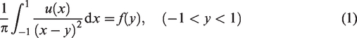
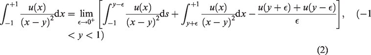
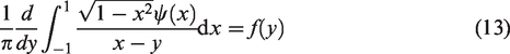
Here, f(y) and u(x) are presented as a known function and an unknown function on the finite interval $(-1,1)$ considering the end points conditions $u(\pm 1)=0$ . In equation (1) the sense of Hadamard finite part is given by ¹⁸

$${\displaystyle {\int }_{-1}^{+1}\frac{u(x)}{{(x-y)}^2}}\text{d}x=\underset{\mathrm{ϵ}\to 0^{+}}{\lim }[{\displaystyle {\int }_{-1}^{y-\mathrm{ϵ}}\frac{u(x)}{{(x-y)}^2}}\text{d}s+{\displaystyle {\int }_{y+\mathrm{ϵ}}^{+1}\frac{u(x)}{{(x-y)}^2}}\text{d}x-\frac{u(y+\mathrm{ϵ})+u(y-\mathrm{ϵ})}{\mathrm{ϵ}}],(-1<y<1)$$

(2)

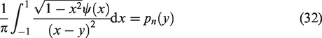
The following equation can be useful in clarifying the exact solution of equation (1) which has been referred in literature.^16,17

$$u(y)=\frac{1}{\pi }{\displaystyle {\int }_{-1}^{+1}f}(x)\ln \left|\frac{y-x}{1-\mathit{yx}+\sqrt{(1-y^2)(1-x^2)}}\right|\text{d}x,(-1<y<1)$$

(3)

We may say that, in equation (3), evaluating the exact solution could be successful.

Obviously, in the case of evaluating the approximate solution of the hypersingular integral equations, plenty of methods need to be prepared.^19–33 To improve a solution to a general hypersingular integral equation of the first kind, one simple but precise approximation method is chosen and investigated in Mandal and Bera. ³⁴ Consideration should be given to the kernel which should be divided to hypersingular and regular parts.

The solution of Cauchy type of singular integral equation in two disjointed intervals has been employed by Dutta and Banerjea ³⁵ to solve a hypersingular integral equation in two intervals. On the other hand, Chen and Zhou ³⁶ took account of an efficient method to adequately solve hypersingular integral equation of the first kind. In reproducing kernel space, they aim to disestablish the singularity of the equation. The rough solutions for hypersingular kernels and Fredholm integral equation of second kind have been achieved by Mandal and Bhattacharya ¹⁵ using Bernstein polynomials as a basis. Mahmoudi ³⁷ actually formed a new modified Adomian decomposition method to solve a class of hypersingular integral equations of the second kind. Also, Eshkuvatov et al. ¹³ have presented a work regarding to the modified homotopy perturbation method for solving hypersingular integral equations of the first kind. In the present paper, we consider the method mentioned in literature^33,37 and then determine a new modified homotopy perturbation method to actually solve hypersingular integral equation of the first kind. The validity and reliability of the new method is not in question and it is simple to be used. To achieve the goals of the paper, we proceed as follows:

In the Preliminaries section, the preliminaries of solving equation (1) by applying the homotopy perturbation method are discussed. In the Modification of the Homotopy Perturbation Method section, identifying the perspective, a new modified homotopy perturbation method is introduced to obtain the solution of equation (1). The Illustrative examples section dedicates to reveal the simplicity and efficiency of the MHPM by solving some sample examples through the proposed algorithm. In the last, the conclusion remarks are placed in the Conclusion section.

Preliminaries

As time passes, new methods are created and others fall into disfavor. He ³⁸ has observed the homotopy perturbation method which recently has been employed in the literature for seeking the solution to linear and nonlinear problems. We do believe that the HPM aims at coupling a homotopy technique of topology and a perturbation technique.^38–46 Some of the recent developments of the HPM have been discussed in literature^47–52 and references therein.

In this work, the proposed scheme is derived and provided in, in essence, bunch of relevant equations which were efficiently taken care of. We should also acknowledge that the coupling of the perturbation method and the homotopy method has been successful in dropping the limitations of the traditional perturbation technique. Accordingly, by using the HPM, we are able to deal with the hypersingular integral equations of the first kind.

Speaking of the basic ideas, the HPM is likely to be discussed by looking at the following equation

$$A(u(y))-f(x)=0,(x\in \Omega )$$

(4)

Embedding the boundary condition

$$B\left(y,\frac{\partial y}{\partial x}\right)=0,(y\in \Gamma )$$

(5)

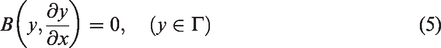
where A, B, f(x), Γ would be called the general differential operator, a boundary operator, a known analytical function and the boundary of the domain Ω, respectively. Two parts are provided having operator A, namely, L (linear) and N(nonlinear). Following this, equation (4) is broken down to the following

$$L(y)+N(y)-f(x)=0$$

(6)

We, on the other hand, may need to establish a homotopy to equation (4), $H(y,p):\Omega \times [0,1]\to \mathbb{R}$ , which for $x\in \Omega$ satisfies

$$\begin{array}{l}H(y,p)=(1-p)[L(y)-L(u_0)]+p[A(y)-f(x)]=0\hfill \end{array}$$

(7)

which is equivalent to

$$H(y,p)=L(y)-L(u_0)+\mathit{pL}(u_0)+p[N(y)-f(x)]=0$$

(8)

where $p\in [0,1]$ is designed to be an embedding parameter and u₀ is regarded to be an initial approximation which fulfills the boundary condition (5). That is, it is acceptable to take equation (8) as

$$\begin{array}{l}H(y,0)=L(y)-L(u_0)=0,\text{and}\hfill \\ H(y,1)=A(y)-f(x)=0\hfill \end{array}$$

(9)

From one point of view, the process of p is turning from 0 into 1 is just that of y(x, p) from $u_0(x)$ to u(x). In topology, that would be called deformation and $L(y)-L(u_0)$ and $A(y)-f(x)$ are called homotopic. Besides, the embedding parameter is expected to be defined much more tangible and unaffected by introducing artificial factors; further we shall consider that as a small parameter for $0 \mathrm{⩽} p\mathrm{⩽}1$ . The solution of equation (7), in turn, should attempt to be stressed as

$$y(x,p)=u_0(x)+p{u}_1(x)+p^2{u}_2(x)+\cdots .$$

(10)

Certainly, in making a decision on substituting equation (10) into equation (8) and jumping to new results in terms of relative emphasis placed on powers of p, an infinite number of differential equation is determined. Now, the solution to this simple differential equation with proper initial conditions is then promised. This process is directed in such a way that an approximate solution to equation (4) is introduced as^53–55

$$y\approx {\displaystyle \sum _{i=0}^m{u}_i}=u_0+u_1+\cdots +u_m$$

(11)

The convergence of series equation (10) as $p\to 1$ has been envisaged by He.^38,39

In equation (1), it is considered that

$$u(y)=\sqrt{1-y^2}\psi (y)$$

(12)

where $\psi (y)$ is supposed to be a smooth function. ¹⁸ By replacing equation (12) into equation (1), we state

$$\frac{1}{\pi }\frac{d}{\mathit{dy}}{\displaystyle {\int }_{-1}^1\frac{\sqrt{1-x^2}\psi (x)}{x-y}}\text{d}x=f(y)$$

(13)

Then, the following definition is required

$$D_j={\displaystyle {\int }_{-1}^{+1}\frac{\sqrt{1-x^2}}{x-y}}{x}^j\text{d}x,(j=0,1,2,\dots )$$

(14)

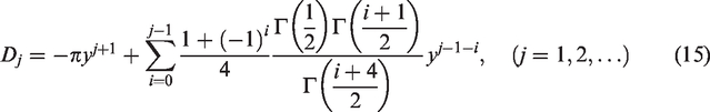
where from Mandal and Bera, ³⁴ it is essential that we have

$$\begin{array}{l}{D}_j=-\pi y^{j+1}+{\displaystyle \sum _{i=0}^{j-1}\frac{1+{(-1)}^i}{4}}\frac{\Gamma \left(\frac{1}{2}\right)\Gamma \left(\frac{i+1}{2}\right)}{\Gamma \left(\frac{i+4}{2}\right)}{y}^{j-1-i},\hspace{1em}(j=1,2,\dots )\hfill \end{array}$$

(15)

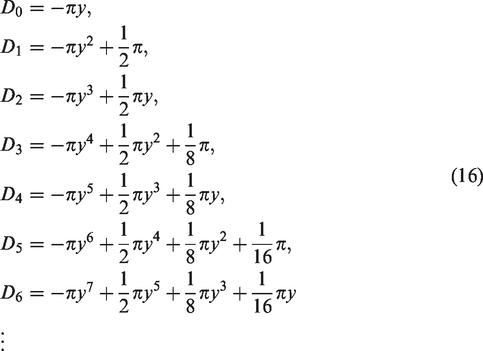
Here, some of the first D_j’s can be stated as follows

$$\begin{array}{l}{D}_0=-\pi y,\hfill \\ D_1=-\pi y^2+\frac{1}{2}\pi ,\hfill \\ D_2=-\pi y^3+\frac{1}{2}\pi y,\hfill \\ D_3=-\pi y^4+\frac{1}{2}\pi y^2+\frac{1}{8}\pi ,\hfill \\ D_4=-\pi y^5+\frac{1}{2}\pi y^3+\frac{1}{8}\pi y,\hfill \\ D_5=-\pi y^6+\frac{1}{2}\pi y^4+\frac{1}{8}\pi y^2+\frac{1}{16}\pi ,\hfill \\ D_6=-\pi y^7+\frac{1}{2}\pi y^5+\frac{1}{8}\pi y^3+\frac{1}{16}\pi y\hfill \\ ⋮\hfill \end{array}$$

(16)

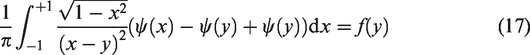
Likewise, applying the new method, the hypersingular integral equations of the first kind mentioned in equation (13) is appropriate to be transformed into the second kind. Such being the case, we may have the following problem

$$\frac{1}{\pi }{\displaystyle {\int }_{-1}^{+1}\frac{\sqrt{1-x^2}}{{(x-y)}^2}}(\psi (x)-\psi (y)+\psi (y))\text{d}x=f(y)$$

(17)

Of course equation (17) is being transformed into the following

$$\begin{array}{l}\frac{1}{\pi }{\displaystyle {\int }_{-1}^{+1}\frac{\sqrt{1-x^2}}{{(x-y)}^2}}\psi (y)\text{d}x=f(y)-\frac{1}{\pi }{\displaystyle {\int }_{-1}^{+1}\frac{\sqrt{1-x^2}}{{(x-y)}^2}}(\psi (x)-\psi (y))\text{d}x\hfill \end{array}$$

(18)

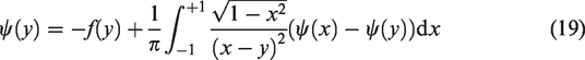
Thus, we announce

$$\psi (y)=-f(y)+\frac{1}{\pi }{\displaystyle {\int }_{-1}^{+1}\frac{\sqrt{1-x^2}}{{(x-y)}^2}}(\psi (x)-\psi (y))\text{d}x$$

(19)

Now, the HPM is considered to be applied to create a solution to equation (19) which is an integral equation of the second kind. To do so, consider the following

$$\psi (y)={\displaystyle \sum _{m=0}^{\infty }{\psi }_m}(y)$$

(20)

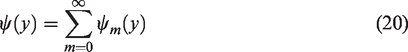
Now, by applying the HPM on equation (19), it is advisable to suppose

$$L\psi =\psi , D\psi =\frac{1}{\pi }{\displaystyle {\int }_{-1}^{+1}\frac{\sqrt{1-x^2}}{{(x-y)}^2}}(\psi (x)-\psi (y))\text{d}x$$

(21)

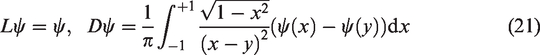
Along the same line, we can rewrite equation (19) to the operator form as follows

$$L\psi -D\psi +f=0$$

(22)

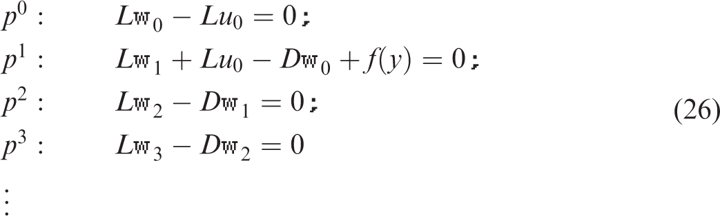
Now, it is also recommended that, we define the homotopy equation (7) as

$$H(\psi ,p)=(1-p)[L\psi -L{u}_0]+p[L\psi -D\psi +f(y)]=0$$

(23)

Assuming

$$\psi ={\psi }_0+{\psi }_{1}p+{\psi }_2{p}^2+{\psi }_3{p}^3+\cdots$$

(24)

Then, substituting this in equation (23) we get

$$\begin{array}{l}(1-p)\left[L({\psi }_0+{\psi }_{1}p+{\psi }_2{p}^2+{\psi }_3{p}^3+\cdots )-L{u}_0\right]\hfill \\ +p[L({\psi }_0+{\psi }_{1}p+{\psi }_2{p}^2+{\psi }_3{p}^3+\cdots )-D({\psi }_0+{\psi }_{1}p+{\psi }_2{p}^2+{\psi }_3{p}^3+\cdots )+f(y)]=0\hfill \end{array}$$

(25)

Therefore, we obtain

$$\begin{array}{l}{p}^0: L{\psi }_0-L{u}_0=0,\hfill \\ p^1: L{\psi }_1+L{u}_0-D{\psi }_0+f(y)=0,\hfill \\ p^2: L{\psi }_2-D{\psi }_1=0,\hfill \\ p^3: L{\psi }_3-D{\psi }_2=0\hfill \\ ⋮\hfill \end{array}$$

(26)

On the other hand, we write down

$$\begin{array}{l}{\psi }_0=u_0,\hfill \\ {\psi }_1=-u_0+D{\psi }_0-f(y),\hfill \\ {\psi }_2=D{\psi }_1,\hfill \\ {\psi }_3=D{\psi }_2,\hfill \\ ⋮\hfill \\ {\psi }_m=D{\psi }_{m-1}, m\ge 2\hfill \end{array}$$

(27)

having equation (21), since L is the identity operator, we can jump to the conclusion that $u_0=0$ .

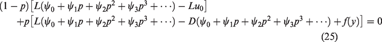
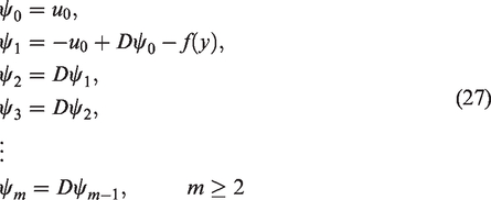
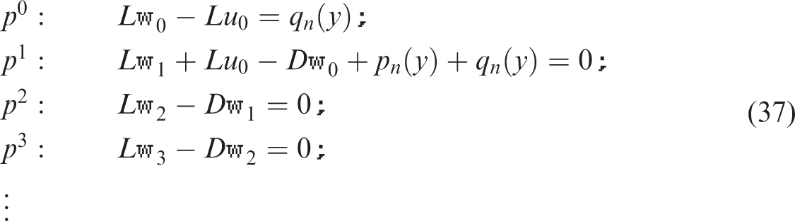
Performing the modified homotopy perturbation method (MHPM) should be carefully done to ensure that we are able to expand $f(y)=f_1(y)+f_2(y)$ and establish the homotopy as follows

$$\begin{array}{l}H(\psi ,p)=(1-p)[L\psi -L{u}_0]+p[L\psi -D\psi +f_2(y)]=-f_1(y)\hfill \end{array}$$

(28)

After substituting equation (24) and simplification, it can be obtained

$$\begin{array}{l}{p}^0: L{\psi }_0-L{u}_0=-f_1(y),\hfill \\ p^1: L{\psi }_1+L{u}_0-D{\psi }_0+f_2(y)=0,\hfill \\ p^2: L{\psi }_2-D{\psi }_1=0,\hfill \\ p^3: L{\psi }_3-D{\psi }_2=0,\hfill \\ ⋮\hfill \end{array}$$

(29)

which provides

$$\begin{array}{l}{\psi }_0=u_0-f_1(y),\hfill \\ {\psi }_1=-u_0+D{\psi }_0-f_2(y),\hfill \\ {\psi }_2=D{\psi }_1,\hfill \\ {\psi }_3=D{\psi }_2,\hfill \\ ⋮\hfill \\ {\psi }_m=D{\psi }_{m-1}, m\ge 2\hfill \end{array}$$

(30)

Let us emphasize that selecting the functions f₁ and f₂ is a very vital task to understand the rate of convergence of the MHPM. In fact, they should be chosen in such a way that ${\psi }_1={\psi }_2=\cdots =0$ . Not any functions can make a suitable performance of the MHPM.

In order to increase the rate of convergence, f₁ and f₂ need to be chosen wisely. In the case that f(y) is a polynomial, the new method is going to be employed. The MHPM is required to be named in which to be helpful in choosing f₁ and f₂ conveniently.

Modification of the homotopy perturbation method

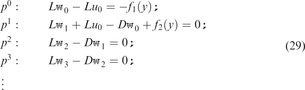
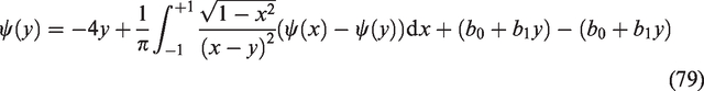
Based on the assumption that the function f can be broken down into two parts, such as f₁ and f₂, the modified form of the HPM was established. Having this assumption we can write

$$f=f_1+f_2$$

As mentioned above, selecting the functions f₁ and f₂ is a very vital task to understand the rate of convergence of the MHPM. Still there are not such rules to be followed. Now,using Mahmoudi ³⁷ in two manners will give us the best resultswhere f in equation (1) is either a polynomial or a non-polynomial analytic function, such procedure should be accomplished as follows.

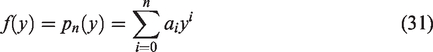
Case I: Let f be a polynomial of degree n.

We employ the new method for the case that f(y) be a polynomial.

Thus

$$f(y)=p_n(y)={\displaystyle \sum _{i=0}^n{a}_i}{y}^i$$

(31)

Equation (1) is altered into equation (31). Having equation (12), we get

$$\frac{1}{\pi }{\displaystyle {\int }_{-1}^1\frac{\sqrt{1-x^2}\psi (x)}{{(x-y)}^2}}\text{d}x=p_n(y)$$

(32)

Then, considering equation (19), we state

$$\psi (y)=-p_n(y)+\frac{1}{\pi }{\displaystyle {\int }_{-1}^{+1}\frac{\sqrt{1-x^2}}{{(x-y)}^2}}(\psi (x)-\psi (y))\text{d}x$$

(33)

At the same time, we add $q_n(y)$ and subtract to the left side of equation (33).

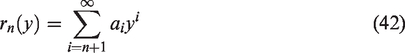
Now, we have

$$\begin{array}{l}\psi (y)=-p_n(y)+\frac{1}{\pi }{\displaystyle {\int }_{-1}^{+1}\frac{\sqrt{1-x^2}}{{(x-y)}^2}}(\psi (x)-\psi (y))\text{d}x+q_n(y)-q_n(y)\hfill \end{array}$$

(34)

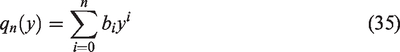
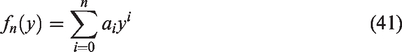
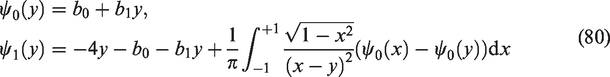
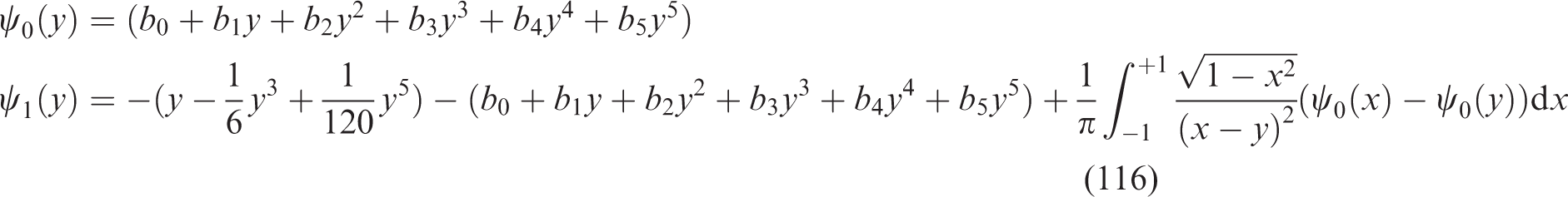
where $q_n(y)$ represents a complete standard form of polynomial with coefficients b_i, $i=0,1,2,\mathrm{\dots }$ equal to the order of polynomial $p_n(y)$ as

$$q_n(y)={\displaystyle \sum _{i=0}^n{b}_i}{y}^i$$

(35)

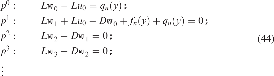
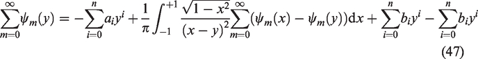
It is considered that, in the HPM, the following relation provides the infinite series of solution for the function which is unknown. When we replace equation (23) with equation (34), it is clear that

$$\begin{array}{l}H(\psi ,p)=(1-p)[L\psi -L{u}_0]+p[L\psi -D\psi +p_n(y)+q_n(y)]=q_n(y)\hfill \end{array}$$

(36)

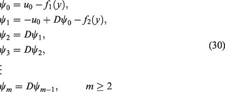
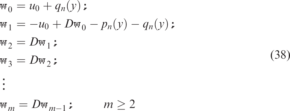
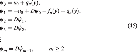
Substituting equation (24) and of course, simplifying, serves the benefit of following set

$$\begin{array}{l}{p}^0: L{\psi }_0-L{u}_0=q_n(y),\hfill \\ p^1: L{\psi }_1+L{u}_0-D{\psi }_0+p_n(y)+q_n(y)=0,\hfill \\ p^2: L{\psi }_2-D{\psi }_1=0,\hfill \\ p^3: L{\psi }_3-D{\psi }_2=0,\hfill \\ ⋮\hfill \end{array}$$

(37)

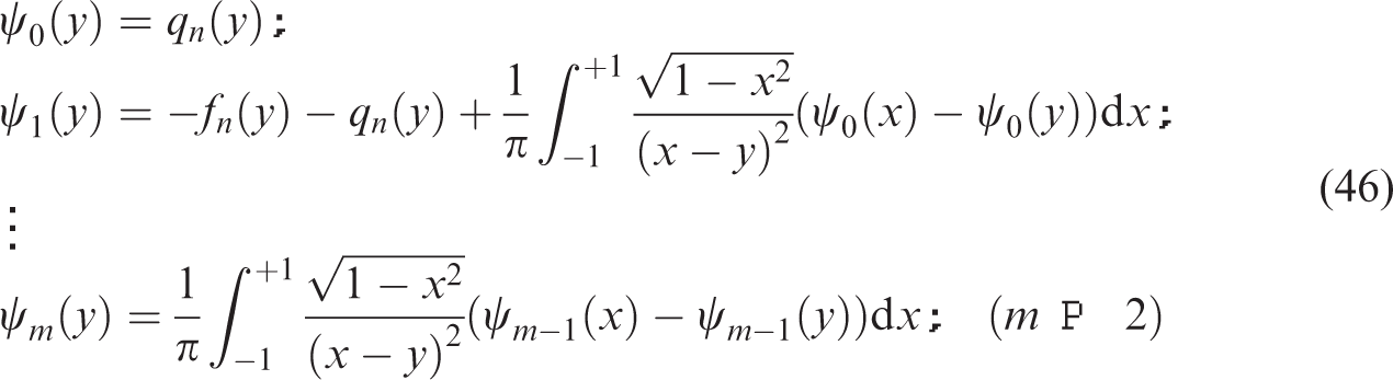
which illustrate

$$\begin{array}{l}{\psi }_0=u_0+q_n(y),\hfill \\ {\psi }_1=-u_0+D{\psi }_0-p_n(y)-q_n(y),\hfill \\ {\psi }_2=D{\psi }_1,\hfill \\ {\psi }_3=D{\psi }_2,\hfill \\ ⋮\hfill \\ {\psi }_m=D{\psi }_{m-1}, m\ge 2\hfill \end{array}$$

(38)

It seems very important to note that, the rate of convergence of the MHPM depends on selecting the functions f₁ and f₂. They are usually chosen in such a way that ${\psi }_1={\psi }_2=\cdots =0$ . In performing the MHPM, of course, it is difficult to choose f₁ and f₂ in such a way that the rate of convergence could be increased. To be clear on determining the method, we set

$$\begin{array}{l}{\psi }_0(y)=q_n(y),\hfill \\ {\psi }_1(y)=-p_n(y)-q_n(y)+\frac{1}{\pi }{\displaystyle {\int }_{-1}^{+1}\frac{\sqrt{1-x^2}}{{(x-y)}^2}}({\psi }_0(x)-{\psi }_0(y))\text{d}x,\hfill \\ ⋮\hfill \\ {\psi }_m(y)=\frac{1}{\pi }{\displaystyle {\int }_{-1}^{+1}\frac{\sqrt{1-x^2}}{{(x-y)}^2}}({\psi }_{m-1}(x)-{\psi }_{m-1}(y))\mathit{dx},(m \mathrm{⩾} 2)\hfill \end{array}$$

(39)

The unknown coefficients of the polynomial $q_n(y)$ is promised by solving ${\psi }_1(y)=0$ , through the fact that f is a polynomial, the exact solution is obtained with no error around. In comparison with the HPM, two terms of the series are calculated. Thus, in this method calculating and finding the solutions are straightforward. The MHPM is applied to some examples; therefore, the capability of this method will be noticed. Note that the method of standard HPM to solve equation (32) converges if f is a polynomial of degree zero, otherwise diverges.

Case II: Let f not be a polynomial.

Through Taylor series expansion of a function, assume that

$$f(y)=f_n(y)+r_n(y)$$

(40)

where

$$f_n(y)={\displaystyle \sum _{i=0}^n{a}_i}{y}^i$$

(41)

$$r_n(y)={\displaystyle \sum _{i=n+1}^{\infty }{a}_i}{y}^i$$

(42)

It can be stated that, $f(y)\simeq f_n(y)$ , now we can elicit from equation (34) as follows

$$\begin{array}{l}H(\psi ,p)=(1-p)[L\psi -L{u}_0]+p[L\psi -D\psi +f_n(y)+q_n(y)]=q_n(y)\hfill \end{array}$$

(43)

where $q_n(y)$ , whose formula is mentioned in equation (35), refers to a complete standard form of polynomial equal to the order of polynomial $f_n(y)$ .

Substituting equation (24) and of course, simplifying, serves the benefit of following set

$$\begin{array}{l}{p}^0: L{\psi }_0-L{u}_0=q_n(y),\hfill \\ p^1: L{\psi }_1+L{u}_0-D{\psi }_0+f_n(y)+q_n(y)=0,\hfill \\ p^2: L{\psi }_2-D{\psi }_1=0,\hfill \\ p^3: L{\psi }_3-D{\psi }_2=0,\hfill \\ ⋮\hfill \end{array}$$

(44)

which gives

$$\begin{array}{l}{\psi }_0=u_0+q_n(y),\hfill \\ {\psi }_1=-u_0+D{\psi }_0-f_n(y)-q_n(y),\hfill \\ {\psi }_2=D{\psi }_1,\hfill \\ {\psi }_3=D{\psi }_2,\hfill \\ ⋮\hfill \\ {\psi }_m=D{\psi }_{m-1}, m\ge 2\hfill \end{array}$$

(45)

In Taylor series expansion of the function for f(y) in equations (41), (45) and (45), the function we get depends on choosing point n that can be written as

$$\begin{array}{l}{\psi }_0(y)=q_n(y),\hfill \\ {\psi }_1(y)=-f_n(y)-q_n(y)+\frac{1}{\pi }{\displaystyle {\int }_{-1}^{+1}\frac{\sqrt{1-x^2}}{{(x-y)}^2}}({\psi }_0(x)-{\psi }_0(y))\text{d}x,\hfill \\ ⋮\hfill \\ {\psi }_m(y)=\frac{1}{\pi }{\displaystyle {\int }_{-1}^{+1}\frac{\sqrt{1-x^2}}{{(x-y)}^2}}({\psi }_{m-1}(x)-{\psi }_{m-1}(y))\text{d}x,\hspace{1em}(m \mathrm{⩾} 2)\hfill \end{array}$$

(46)

The unknown coefficients of the polynomial $q_n(y)$ will be provided by reaching the solution to ${\psi }_1(y)=0$ .

Lemma 1. Let f in equation (1) be a polynomial of degree n, and considering $f(y)={\sum }_{i=0}^n{a}_i{y}^i$ , and using the MHPM, the exact solution of equation (32) is obtained.

Proof. If f in equation (1) is a polynomial of degree n, as in equation (40) then, considering equation (46), in this case we say that

$$\begin{array}{l}{\displaystyle \sum _{m=0}^{\infty }{\psi }_m}(y)=-{\displaystyle \sum _{i=0}^n{a}_i}{y}^i+\frac{1}{\pi }{\displaystyle {\int }_{-1}^{+1}\frac{\sqrt{1-x^2}}{{(x-y)}^2}}{\displaystyle \sum _{m=0}^{\infty }({\psi }_m(x)-{\psi }_m(y))}\text{d}x+{\displaystyle \sum _{i=0}^n{b}_i}{y}^i-{\displaystyle \sum _{i=0}^n{b}_i}{y}^i\hfill \end{array}$$

(47)

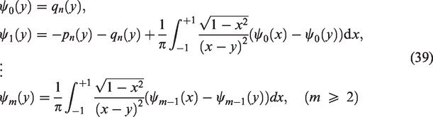
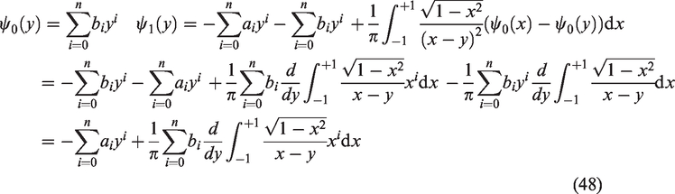
By understanding equation (46), we equip with the following statement

$$\begin{array}{l}{\psi }_0(y)={\displaystyle \sum _{i=0}^n{b}_i}{y}^i{\psi }_1(y)=-{\displaystyle \sum _{i=0}^n{a}_i}{y}^i-{\displaystyle \sum _{i=0}^n{b}_i}{y}^i+\frac{1}{\pi }{\displaystyle {\int }_{-1}^{+1}\frac{\sqrt{1-x^2}}{{(x-y)}^2}}({\psi }_0(x)-{\psi }_0(y))\text{d}x\\ \hspace{1em}\hspace{0.17em}\hspace{0.17em}\hspace{1em}=-{\displaystyle \sum _{i=0}^n{b}_i}{y}^i-{\displaystyle \sum _{i=0}^n{a}_i}{y}^i+\frac{1}{\pi }{\displaystyle \sum _{i=0}^n{b}_i}\frac{d}{dy}{\displaystyle {\int }_{-1}^{+1}\frac{\sqrt{1-x^2}}{x-y}}{x}^i\text{d}x-\frac{1}{\pi }{\displaystyle \sum _{i=0}^n{b}_i}{y}^i\frac{d}{dy}{\displaystyle {\int }_{-1}^{+1}\frac{\sqrt{1-x^2}}{x-y}}\text{d}x\\ \hspace{1em}\hspace{0.17em}\hspace{0.17em}\hspace{1em}=-{\displaystyle \sum _{i=0}^n{a}_i}{y}^i+\frac{1}{\pi }{\displaystyle \sum _{i=0}^n{b}_i}\frac{d}{dy}{\displaystyle {\int }_{-1}^{+1}\frac{\sqrt{1-x^2}}{x-y}}{x}^i\text{d}x\end{array}$$

(48)

Considering the nature of the MHPM with respect to ${\psi }_1(y)=0$ lies in the system n + 1 leading to

$$\frac{1}{\pi }{\displaystyle \sum _{i=0}^n{b}_i}\frac{d}{dy}{\displaystyle {\int }_{-1}^{+1}\frac{\sqrt{1-x^2}}{x-y}}{x}^i\text{d}x={\displaystyle \sum _{i=0}^n{a}_i}{y}^i$$

(49)

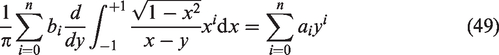
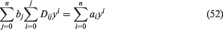
where we regard a_i as known and b_i as unknown ( $i=0,1,\dots ,n$ ) through the system which required to be determined. Now, to reach the values to a_i and b_i, we should go through the following term

$${\displaystyle \sum _{j=0}^n{b}_j}\frac{1}{\pi }\frac{d}{dy}︸\underset{\underset{D_j(y)}{{\displaystyle {\int }_{-1}^1\frac{\sqrt{1-x^2}}{x-y}}{x}^j\text{d}x}}{\hspace{0.17em}}={\displaystyle \sum _{i=0}^n{a}_i}{y}^i$$

(50)

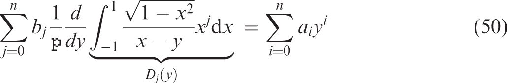
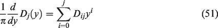
Presenting that $D_j(y)$ is a polynomial of order j + 1, the following statement is valid

$$\frac{1}{\pi }\frac{d}{dy}{D}_j(y)={\displaystyle \sum _{i=0}^j{D}_{\mathit{ij}}}{y}^i$$

(51)

where the formula $D_{\mathit{ij}}={\frac{1}{\pi }\frac{1}{i!}\frac{d^{i+1}}{d{y}^{i+1}}{D}_j(y)|}_{y=0}$ makes it possible to the coefficient yⁱ in $\frac{1}{\pi }\frac{d}{dy}{D}_j(y)$ .

Substituting equation (51) by equation (50), we obtain

$${\displaystyle \sum _{j=0}^n{b}_j}{\displaystyle \sum _{i=0}^j{D}_{\mathit{ij}}}{y}^i={\displaystyle \sum _{i=0}^n{a}_i}{y}^i$$

(52)

Hence

$${\displaystyle \sum _{i=0}^n(}{\displaystyle \sum _{j=i}^n{b}_j}{D}_{\mathit{ij}})y^i={\displaystyle \sum _{i=0}^n{a}_i}{y}^i$$

(53)

Thus

$${\displaystyle \sum _{j=i}^n{b}_j}{D}_{\mathit{ij}}=a_i,(i=0,1,\dots ,n)$$

(54)

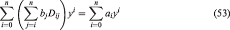
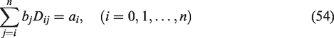
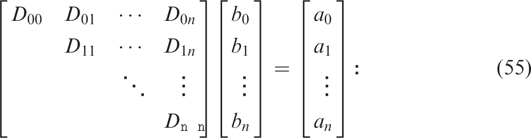
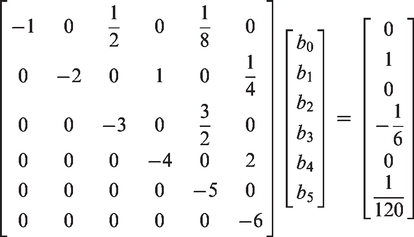
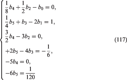
If that was the case, we should think of equation (54) as a linear equation system with an upper triangular coefficient matrix, and it implies

$$\left[\begin{array}{cccc}{D}_{00}& D_{01}& \cdots & D_{0n}\\ & D_{11}& \cdots & D_{1n}\\ & & \ddots & ⋮\\ & & & D_{\mathit{nn}}\end{array}\right]\left[\begin{array}{c}{b}_0\\ b_1\\ ⋮\\ b_n\end{array}\right]=\left[\begin{array}{c}{a}_0\\ a_1\\ ⋮\\ a_n\end{array}\right].$$

(55)

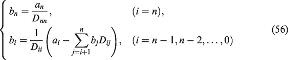
As we are interested in applying backward substitution, equation (55) should be written as follows

$$\begin{array}{l}\{\begin{array}{l}{b}_n=\frac{a_n}{D_{\mathit{nn}}},(i=n),\hfill \\ b_i=\frac{1}{D_{\mathit{ii}}}\left(a_i-{\displaystyle \sum _{j=i+1}^n{b}_j}{D}_{\mathit{ij}}\right),(i=n-1,n-2,\dots ,0)\hfill \end{array}\hfill \end{array}$$

(56)

Having $D_{\mathit{ij}}={\frac{1}{\pi }\frac{1}{i!}\frac{{\text{d}}^{i+1}}{\text{d}{y}^{i+1}}{D}_j(y)|}_{y=0}$ , if i = j, then it is $D_{\mathit{ii}}={\frac{1}{\pi }\frac{1}{i!}\frac{{\text{d}}^{i+1}}{\text{d}{y}^{i+1}}{D}_i(y)|}_{y=0}$ , since $D_i(y)$ is a polynomial of degree i + 1, and consistently $D_{\mathit{ii}}\ne 0$ .

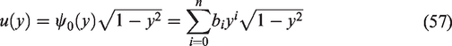
Finally, the exact solution to equation (1) is clarified as follows

$$\begin{array}{c}u(y)={\psi }_0(y)\sqrt{1-y^2}={\displaystyle \sum _{i=0}^n{b}_i}{y}^i\sqrt{1-y^2}\end{array}$$

(57)

determined the corrections.

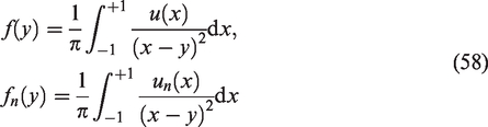
Lemma 2. If f is an analytic function and, subject to $f(y)=f_n(y)+r_n(y)$ , where $f_n(y)$ and $r_n(y)$ are presented as truncated Taylor series of f(y) and the remaining part and $u_n(y)$ respectively, (u_n(y) is the approximate solution of equation (1) obtained from equation (3), then   we have

$$\left|\right|u(y)-u_n(y)\left|\right|\mathrm{⩽}C\left|\right|f(y)-f_n(y)\left|\right|$$

where

$$C\simeq 1.027228877$$

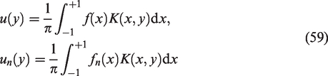
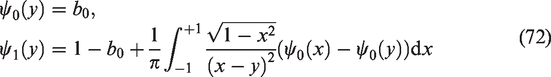
Proof. Let f be an analytic function, and $f(y)=f_n(y)+r_n(y)$ , where $f_n(y)$ is plugged in equation (32), and assuming that $u_n(y)$ is the approximate solution to the MHPM, the following would be written

$$\begin{array}{c}f(y)=\frac{1}{\pi }{\displaystyle {\int }_{-1}^{+1}\frac{u(x)}{{(x-y)}^2}}\text{d}x,\\ f_n(y)=\frac{1}{\pi }{\displaystyle {\int }_{-1}^{+1}\frac{u_n(x)}{{(x-y)}^2}}\text{d}x\end{array}$$

(58)

Considering equation (3) we meet

$$\begin{array}{l}u(y)=\frac{1}{\pi }{\displaystyle {\int }_{-1}^{+1}f}(x)K(x,y)\text{d}x,\\ u_n(y)=\frac{1}{\pi }{\displaystyle {\int }_{-1}^{+1}{f}_n}(x)K(x,y)\text{d}x\end{array}$$

(59)

where

$$K(x,y)=\ln \left|\frac{y-x}{1-\mathit{yx}+\sqrt{(1-y^2)(1-x^2)}}\right|$$

(60)

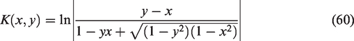
By supporting the idea of subtracting both sides of equation (59), the following is recommended to be made

$$u(y)-u_n(y)=\frac{1}{\pi }{\displaystyle {\int }_{-1}^{+1}(f(}x)-f_n(x))K(x,y)\text{d}x$$

(61)

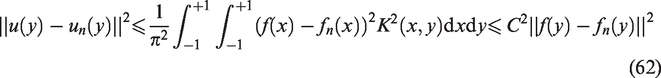
Furthermore, based on the integration of both sides with respect to t that lies in the interval $(-1,+1)$ and employing Cauchy-Schwarz inequality, the following relation is obtained

$$\begin{array}{l}\left|\right|u(y)-u_n(y)|{|}^2\mathrm{⩽}\frac{1}{{\pi }^2}{\displaystyle {\int }_{-1}^{+1}{\displaystyle {\int }_{-1}^{+1}(f(}}x)-f_n(x){)}^2{K}^2(x,y)\text{d}x\text{d}y\mathrm{⩽}{C}^2\left|\right|f(y)-f_n(y)|{|}^2\end{array}$$

(62)

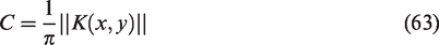
where

$$C=\frac{1}{\pi }\left|\right|K(x,y)\left|\right|$$

(63)

Note that the norm used in the computation is of the L₂ and assistance of numerical integration MAPLE software has been employed. Then, checking equation (60), the approximate value of C is promised as follows

$$C\simeq 1.027228877$$

(64)

With these pieces of information from the above theorem, when n increases since f_n tends to f, therefore u_n tends to u, too. The following results are obtained.

Corollary 1. If f refers to a polynomial of order n, in equation (1) and finally giving equation (1) the exact solution to equation (32) is supposed to be of degree n.

Corollary 2. If f refers to a polynomial of degree n, however, the approximation error from the MHPM falls to zero.

Illustrative examples

The purpose of this section is to develop some of the most common examples to prepare the overriding characteristics of efficiency and simplicity of the MHPM to provide the appropriate solution to hypersingular integral equations of the first kind. In order to solve the following examples, we have used the MAPLE package throughout the paper.

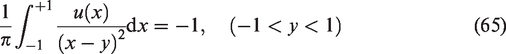
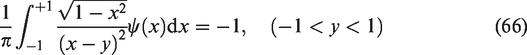
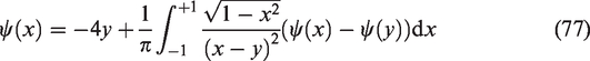
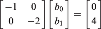
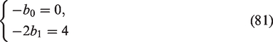
Example 1. Consider the simple hypersingular integral equation of the form ¹⁵ presented

$$\frac{1}{\pi }{\displaystyle {\int }_{-1}^{+1}\frac{u(x)}{{(x-y)}^2}}\text{d}x=-1,(-1<y<1)$$

(65)

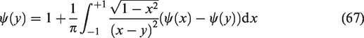
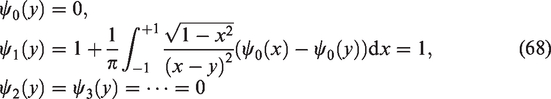
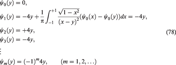
equipped with the additional requirement that $u(\pm 1)=0$ . Running $u(y)=\sqrt{1-y^2}\psi (y)$ , in equation (65) we obtain

$$\frac{1}{\pi }{\displaystyle {\int }_{-1}^{+1}\frac{\sqrt{1-x^2}}{{(x-y)}^2}}\psi (x)\text{d}x=-1,(-1<y<1)$$

(66)

where $f(y)=-1$ refers to a polynomial of zero degree. Now plugging the HPM in equation (66), and checking equation (19) and equation (27) we develop

$$\psi (y)=1+\frac{1}{\pi }{\displaystyle {\int }_{-1}^{+1}\frac{\sqrt{1-x^2}}{{(x-y)}^2}}(\psi (x)-\psi (y))\text{d}x$$

(67)

and

$$\begin{array}{l}{\psi }_0(y)=0,\hfill \\ {\psi }_1(y)=1+\frac{1}{\pi }{\displaystyle {\int }_{-1}^{+1}\frac{\sqrt{1-x^2}}{{(x-y)}^2}}({\psi }_0(x)-{\psi }_0(y))\text{d}x=1,\hfill \\ {\psi }_2(y)={\psi }_3(y)=\cdots =0\hfill \end{array}$$

(68)

Having equation (24) we state

$$\psi (y)={\displaystyle \sum _{m=0}^{\infty }{\psi }_m}(y)=1$$

(69)

Following the steps which are mentioned above is an important task, so we are able to achieve the solution of the integral equation (65) as

$$u(y)=\psi (y)\sqrt{1-y^2}=\sqrt{1-y^2}$$

(70)

which is the exact solution of the integral equation.

Next we use the MHPM in equation (66) along with equation (34) we write

$$\psi (y)=1+\frac{1}{\pi }{\displaystyle {\int }_{-1}^{+1}\frac{\sqrt{1-x^2}}{{(x-y)}^2}}(\psi (x)-\psi (y))\text{d}x+b_0-b_0$$

(71)

By employing the repeated scheme mentioned in equation (39) we now illustrate that

$$\begin{array}{l}{\psi }_0(y)=b_0,\\ {\psi }_1(y)=1-b_0+\frac{1}{\pi }{\displaystyle {\int }_{-1}^{+1}\frac{\sqrt{1-x^2}}{{(x-y)}^2}}({\psi }_0(x)-{\psi }_0(y))\text{d}x\end{array}$$

(72)

By placing ${\psi }_1(y)=0$ , and according to equation (55), the following system is written, $b_0=1$ . And then

$$\psi (y)={\psi }_0(y)=1$$

(73)

and next

$$u(y)=\sqrt{1-y^2}$$

(74)

Example 2. The hypersingular integral equation (1) is supposed to be as ¹⁴

$$\frac{1}{\pi }{\displaystyle {\int }_{-1}^{+1}\frac{u(x)}{{(x-y)}^2}}\text{d}x=4y,(-1<y<1)$$

(75)

By applying u(y), in equation (75) we write

$$\frac{1}{\pi }{\displaystyle {\int }_{-1}^{+1}\frac{\sqrt{1-x^2}}{{(x-y)}^2}}\psi (x)\text{d}x=4y,(-1<y<1)$$

(76)

where $f(y)=4y$ refers to a polynomial of order one, then plugging the HPM in equation (76), and considering equation (19) and equation (27) we get the following

$$\psi (x)=-4y+\frac{1}{\pi }{\displaystyle {\int }_{-1}^{+1}\frac{\sqrt{1-x^2}}{{(x-y)}^2}}(\psi (x)-\psi (y))\text{d}x$$

(77)

and

$$\begin{array}{l}{\psi }_0(y)=0,\hfill \\ {\psi }_1(y)=-4y+\frac{1}{\pi }{\displaystyle {\int }_{-1}^{+1}\frac{\sqrt{1-x^2}}{{(x-y)}^2}}({\psi }_0(x)-{\psi }_0(y))\mathit{dx}=-4y,\hfill \\ {\psi }_2(y)=+4y,\hfill \\ {\psi }_3(y)=-4y,\hfill \\ ⋮\hfill \\ {\psi }_m(y)={(-1)}^{m}4y,(m=1,2,\dots )\hfill \end{array}$$

(78)

which is written as a divergent series.

Employing the MHPM in equation (75) along with equation (34) we write

$$\begin{array}{c}\psi (y)=-4y+\frac{1}{\pi }{\displaystyle {\int }_{-1}^{+1}\frac{\sqrt{1-x^2}}{{(x-y)}^2}}(\psi (x)-\psi (y))\text{d}x+(b_0+b_{1}y)-(b_0+b_{1}y)\end{array}$$

(79)

By employing the repeated scheme equation (39), we now illustrate that

$$\begin{array}{l}{\psi }_0(y)=b_0+b_{1}y,\\ {\psi }_1(y)=-4y-b_0-b_{1}y+\frac{1}{\pi }{\displaystyle {\int }_{-1}^{+1}\frac{\sqrt{1-x^2}}{{(x-y)}^2}}({\psi }_0(x)-{\psi }_0(y))\text{d}x\end{array}$$

(80)

By placing ${\psi }_1(y)=0$ , and according to equation (55), the following system is written

$$\left[\begin{array}{cc}-1& 0\\ 0& -2\end{array}\right]\left[\begin{array}{c}{b}_0\\ b_1\end{array}\right]=\left[\begin{array}{c}0\\ 4\end{array}\right]$$

Given equation (56), we find

$$\{\begin{array}{l}-b_0=0,\hfill \\ -2b_1=4\hfill \end{array}$$

(81)

Having $b_1=-2$ and $b_0=0$ , then

$$\psi (y)={\psi }_0(y)=-2y$$

(82)

next

$$u(y)=(-2y)\sqrt{1-y^2}$$

(83)

Example 3. Considering the following hypersingular integral equation of the first kind ¹⁷

$$\frac{1}{\pi }{\displaystyle {\int }_{-1}^{+1}\frac{u(x)}{{(x-y)}^2}}\text{d}x=-(3y^2+\frac{1}{2}),(-1<y<1)$$

(84)

Plugging $u(y)=\sqrt{1-y^2}\psi (y)$ in equation (84), it is written as

$$\frac{1}{\pi }{\displaystyle {\int }_{-1}^{+1}\frac{\sqrt{1-x^2}}{{(x-y)}^2}}\psi (x)\text{d}x=-(3y^2+\frac{1}{2}),(-1<y<1)$$

(85)

where $f(y)=-\left(3y^2+\frac{1}{2}\right)$ , to be a polynomial of order 2. Now plugging the HPM in equation (85), and having equations (19) and (27) it is illustrated that

$$\psi (y)=3y^2+\frac{1}{2}+\frac{1}{\pi }{\displaystyle {\int }_{-1}^{+1}\frac{\sqrt{1-x^2}}{{(x-y)}^2}}(\psi (x)-\psi (y))\text{d}x$$

(86)

and

$$\begin{array}{l}{\psi }_0(y)=0,\\ {\psi }_1(y)=3y^2+\frac{1}{2}+\frac{1}{\pi }{\displaystyle {\int }_{-1}^{+1}\frac{\sqrt{1-x^2}}{{(x-y)}^2}}({\psi }_0(x)-{\psi }_0(y))\text{d}x=3y^2+\frac{1}{2},\\ {\psi }_2(y)=6y^2+\frac{3}{2},\\ {\psi }_3(y)=12y^2-3,\\ ⋮\end{array}$$

(87)

Then employing equation (24) we consider

$$\begin{array}{c}\psi (y)={\displaystyle \sum _{m=0}^{\infty }{\psi }_m}(y)=(3-6+12+\cdots )y^2+\left(\frac{1}{2}+\frac{3}{2}-3+\cdots \right)\end{array}$$

(88)

Which is known as a divergent series.

And next, utilizing the MHPM to equation (85) along with equation (34), we write

$$\begin{array}{c}\psi (y)=3y^2+\frac{1}{2}+\frac{1}{\pi }{\displaystyle {\int }_{-1}^{+1}\frac{\sqrt{1-x^2}}{{(x-y)}^2}}(\psi (x)-\psi (y))\text{d}x+\left(b_0+b_{1}y+b_2{y}^2\right)-\left(b_0+b_{1}y+b_2{y}^2\right)\end{array}$$

(89)

By employing the recursive scheme in equation (39), we now illustrate that

$$\begin{array}{l}{\psi }_0(y)=(b_0+b_{1}y+b_2{y}^2),\\ {\psi }_1(y)=3y^2+\frac{1}{2}-(b_0+b_{1}y+b_2{y}^2)+\frac{1}{\pi }{\displaystyle {\int }_{-1}^{+1}\frac{\sqrt{1-x^2}}{{(x-y)}^2}}({\psi }_0(x)-{\psi }_0(y))\text{d}x\end{array}$$

(90)

By placing ${\psi }_1(y)=0$ , and according to equation (55), the following system is written

$$\left[\begin{array}{ccc}-1& 0& \frac{1}{2}\\ 0& -2& 0\\ 0& 0& -3\end{array}\right]\left[\begin{array}{c}{b}_0\\ b_1\\ b_2\end{array}\right]=\left[\begin{array}{c}-\frac{1}{2}\\ 0\\ -3\end{array}\right]$$

Given equation (56), we get

$$\{\begin{array}{l}-b_0+\frac{1}{2}{b}_2=-\frac{1}{2},\hfill \\ -2b_1=0,\hfill \\ -3b_2=-3\hfill \end{array}$$

(91)

Giving $b_2=1,b_1=0$ and $b_0=1$ , then

$$\psi (y)={\psi }_0(y)=1+y^2$$

(92)

next

$$u(y)=(1+y^2)\sqrt{1-y^2}$$

(93)

is the exact solution of equation (84).

Example 4. We consider the following hypersingular integral equation of the first kind ¹⁷

$$\frac{1}{\pi }{\displaystyle {\int }_{-1}^{+1}\frac{u(x)}{{(x-y)}^2}}\text{d}x=8y^3-2y+1,(-1<y<1)$$

(94)

By employing $u(y)=\sqrt{1-y^2}$ in equation (94), we get

$$\frac{1}{\pi }{\displaystyle {\int }_{-1}^{+1}\frac{\sqrt{1-x^2}}{{(x-y)}^2}}\psi (x)\text{d}x=8y^3-2y+1,(-1<y<1)$$

(95)

where $f(y)=8y^3-2y+1$ refers to a polynomial of 3, then plugging the HPM in equation (95), and considering equation (19) and equation (27), so equation (96) would be as follows

$$\psi \left(y\right)=-8y^3+2y-1+\frac{1}{\pi }{\displaystyle {\int }_{-1}^{+1}\frac{\sqrt{1-x^2}}{{\left(x-y\right)}^2}\left(\psi \left(x\right)-\psi \left(y\right)\right)}\text{d}x$$

(96)

and

$$\begin{array}{l}{\psi }_0(y)=0,\\ {\psi }_1(y)=-8y^3+2y-1+\frac{1}{\pi }{\displaystyle {\int }_{-1}^{+1}\frac{\sqrt{1-x^2}}{{(x-y)}^2}}({\psi }_0(x)-{\psi }_0(y))\text{d}x=-8y^3+2y-1,\\ {\psi }_2(y)=-24y^3+10y,\\ {\psi }_3(y)=72y^3+34y,\\ ⋮\end{array}$$

(97)

Then having equation (24) we write

$$\begin{array}{c}\psi (y)={\displaystyle \sum _{m=0}^{\infty }{\psi }_m}(y)=(8-24+72+\cdots )y^3+(-2+10+34+\cdots )y-1\end{array}$$

(98)

which named as a divergent series.

Applying the MHPM to equation (95) along with equation (34), we get

$$\begin{array}{c}\psi (y)=-8y^3+2y-1+\frac{1}{\pi }{\displaystyle {\int }_{-1}^{+1}\frac{\sqrt{1-x^2}}{{(x-y)}^2}}(\psi (x)-\psi (y))\text{d}x+(b_0+b_{1}y+b_2{y}^2+b_3{y}^3)-(b_0+b_{1}y+b_2{y}^2+b_3{y}^3)\end{array}$$

(99)

By employing the iterative scheme in equation (39), we now illustrate that

$$\begin{array}{l}{\psi }_0(y)=(b_0+b_{1}y+b_2{y}^2+b_3{y}^3),\\ {\psi }_1(y)=-8y^3+2y-1-\left(b_0+b_{1}y+b_2{y}^2+b_3{y}^3\right)+\frac{1}{\pi }{\displaystyle {\int }_{-1}^{+1}\frac{\sqrt{1-x^2}}{{(x-y)}^2}}({\psi }_0(x)-{\psi }_0(y))\text{d}x\end{array}$$

(100)

By placing ${\psi }_1(y)=0$ , and according to equation (55), the following system is written

$$\left[\begin{array}{cccc}-1& 0& \frac{1}{2}& 0\\ 0& -2& 0& 1\\ 0& 0& -3& 0\\ 0& 0& 0& -4\end{array}\right]\left[\begin{array}{c}{b}_0\\ b_1\\ b_2\\ b_3\end{array}\right]=\left[\begin{array}{c}1\\ -2\\ 0\\ 8\end{array}\right]$$

Given equation (56), we have

$$\{\begin{array}{l}\frac{1}{2}{b}_2-b_0=1,\hfill \\ b_3-2b_1=-2,\hfill \\ -3b_2=0,\hfill \\ -4b_3=8\hfill \end{array}$$

(101)

Giving $b_3=-2,b_2=0,b_1=0$ and $b_0=-1$ , then

$$\psi (y)={\psi }_0(y)=-2y^3-1$$

(102)

and next

$$u(y)=-(2y^3+1)\sqrt{1-y^2}$$

(103)

Example 5. Let the following hypersingular integral equation of the first kind ¹⁷

$$\frac{1}{\pi }{\displaystyle {\int }_{-1}^{+1}\frac{u(x)}{{(x-y)}^2}}\text{d}x=e^y,(-1<y<1)$$

(104)

where $f(y)=e^y$ expanded using Taylor-polynomial

$$\begin{array}{c}f(y)={\displaystyle \sum _{n=0}^{\infty }\frac{y^n}{n!}}=1+y+\frac{1}{2}{y}^2+\frac{1}{6}{y}^3+\frac{1}{24}{y}^4+\frac{1}{120}{y}^5+\frac{1}{720}{y}^6+\frac{1}{5040}{y}^7+\frac{1}{40320}{y}^8+\cdots \end{array}$$

(105)

Running the MHPM, applying the equation (34) for n = 5, the following statement is written

$$\begin{array}{l}\psi (y)=-\left(1+y+\frac{1}{2}{y}^2+\frac{1}{6}{y}^3+\frac{1}{24}{y}^4+\frac{1}{120}{y}^5\right)+\frac{1}{\pi }{\displaystyle {\int }_{-1}^{+1}\frac{\sqrt{1-x^2}}{{(x-y)}^2}}(\psi (x)-\psi (y))\text{d}x\\ +(b_0+b_{1}y+b_2{y}^2+b_3{y}^3+b_4{y}^4+b_5{y}^5)-(b_0+b_{1}y+b_2{y}^2+b_3{y}^3+b_4{y}^4+b_5{y}^5)\end{array}$$

(106)

By employing the repeated scheme mentioned in equation (46), we can say that

$$\begin{array}{l}{\psi }_0(y)=(b_0+b_{1}y+b_2{y}^2+b_3{y}^3+b_4{y}^4+b_5{y}^5)\hfill \\ {\psi }_1(y)=-\left(1+y+\frac{1}{2}{y}^2+\frac{1}{6}{y}^3+\frac{1}{24}{y}^4+\frac{1}{120}{y}^5\right)-(b_0+b_{1}y+b_2{y}^2+b_3{y}^3+b_4{y}^4+b_5{y}^5)\hfill \\ +\frac{1}{\pi }{\displaystyle {\int }_{-1}^{+1}\frac{\sqrt{1-x^2}}{{(x-y)}^2}}({\psi }_0(x)-{\psi }_0(y))\text{d}x\hfill \end{array}$$

(107)

By placing ${\psi }_1(y)=0$ , and according to equation (55), the following system is written

$$\left[\begin{array}{cccccc}-1& 0& \frac{1}{2}& 0& \frac{1}{8}& 0\\ 0& -2& 0& 1& 0& \frac{1}{4}\\ 0& 0& -3& 0& \frac{3}{2}& 0\\ 0& 0& 0& -4& 0& 2\\ 0& 0& 0& 0& -5& 0\\ 0& 0& 0& 0& 0& -6\end{array}\right]\left[\begin{array}{c}{b}_0\\ b_1\\ b_2\\ b_3\\ b_4\\ b_5\end{array}\right]=\left[\begin{array}{c}1\\ 1\\ \frac{1}{2}\\ \frac{1}{6}\\ \frac{1}{24}\\ \frac{1}{120}\end{array}\right]$$

Given equation (56), we get

$$\{\begin{array}{l}\frac{1}{8}{b}_4+\frac{1}{2}{b}_2-b_0=1,\hfill \\ \frac{1}{4}{b}_5+b_3-2b_1=1,\hfill \\ \frac{3}{2}{b}_4-3b_2=\frac{1}{2},\hfill \\ 2b_5-4b_3=\frac{1}{6},\hfill \\ -5b_4=\frac{1}{24},\hfill \\ -6b_5=\frac{1}{120}\hfill \end{array}$$

(108)

Giving $b_5=-\frac{1}{720},b_4=-\frac{1}{120},b_3=-\frac{61}{1440},b_2=-\frac{41}{240},b_1=-\frac{1001}{1920}$ and $b_0=-\frac{1043}{960}$ , then

$$\psi (y)={\psi }_0(y)=-\left(\frac{1}{720}{y}^5+\frac{1}{120}{y}^4+\frac{61}{1440}{y}^3+\frac{41}{240}{y}^2+\frac{1001}{1920}y+\frac{1043}{960}\right)$$

(109)

and next

$$u_5(y)=-\left(\frac{1}{720}{y}^5+\frac{1}{120}{y}^4+\frac{61}{1440}{y}^3+\frac{41}{240}{y}^2+\frac{1001}{1920}y+\frac{1043}{960}\right)\sqrt{1-y^2}$$

(110)

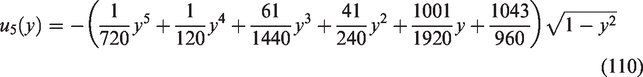
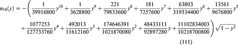
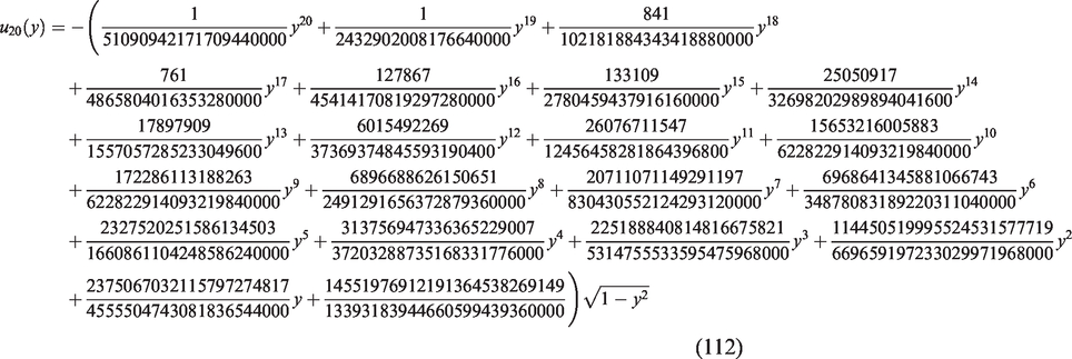
Accordingly, for n = 10 and n = 20, the following statements could be arranged as follows

$$\begin{array}{c}{u}_{10}(y)=-(\frac{1}{39916800}{y}^{10}+\frac{1}{3628800}{y}^9+\frac{221}{79833600}{y}^8+\frac{181}{7257600}{y}^7+\frac{63803}{319334400}{y}^6+\frac{13561}{9676800}{y}^5\\ +\frac{1077253}{127733760}{y}^4+\frac{492013}{11612160}{y}^3+\frac{174646391}{1021870080}{y}^2+\frac{48433111}{92897280}y+\frac{11102834003}{10218700800})\sqrt{1-y^2}\end{array}$$

(111)

$$\begin{array}{l}{u}_{20}(y)=-(\frac{1}{51090942171709440000}{y}^{20}+\frac{1}{2432902008176640000}{y}^{19}+\frac{841}{102181884343418880000}{y}^{18}\\ +\frac{761}{4865804016353280000}{y}^{17}+\frac{127867}{45414170819297280000}{y}^{16}+\frac{133109}{2780459437916160000}{y}^{15}+\frac{25050917}{32698202989894041600}{y}^{14}\\ +\frac{17897909}{1557057285233049600}{y}^{13}+\frac{6015492269}{37369374845593190400}{y}^{12}+\frac{26076711547}{12456458281864396800}{y}^{11}+\frac{15653216005883}{622822914093219840000}{y}^{10}\\ +\frac{172286113188263}{622822914093219840000}{y}^9+\frac{6896688626150651}{2491291656372879360000}{y}^8+\frac{20711071149291197}{830430552124293120000}{y}^7+\frac{6968641345881066743}{34878083189220311040000}{y}^6\\ +\frac{2327520251586134503}{1660861104248586240000}{y}^5+\frac{313756947336365229007}{37203288735168331776000}{y}^4+\frac{225188840814816675821}{5314755533595475968000}{y}^3+\frac{114450519995524531577719}{669659197233029971968000}{y}^2\\ +\frac{2375067032115797274817}{4555504743081836544000}y+\frac{14551976912191364538269149}{13393183944660599439360000})\sqrt{1-y^2}\end{array}$$

(112)

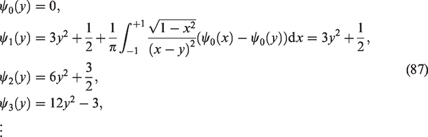
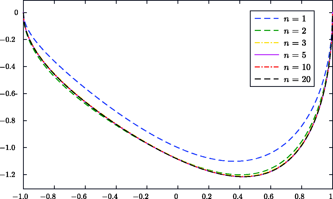
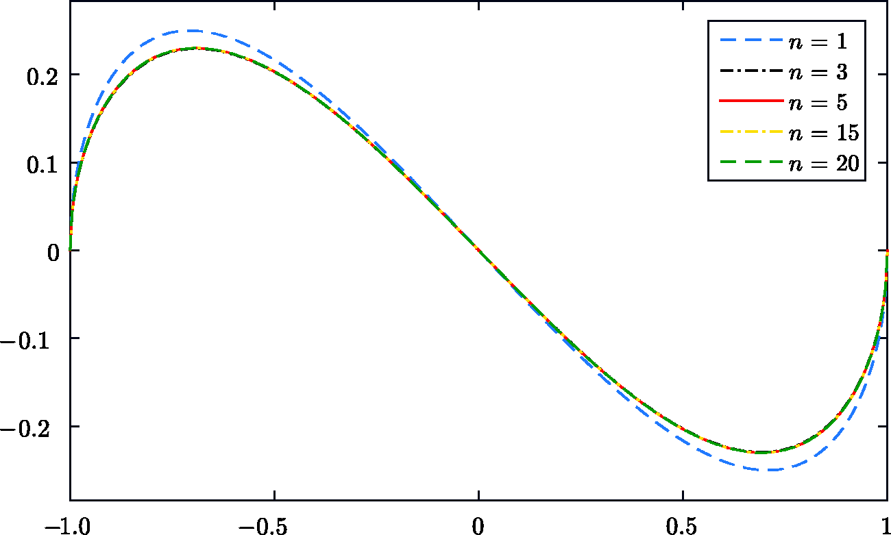
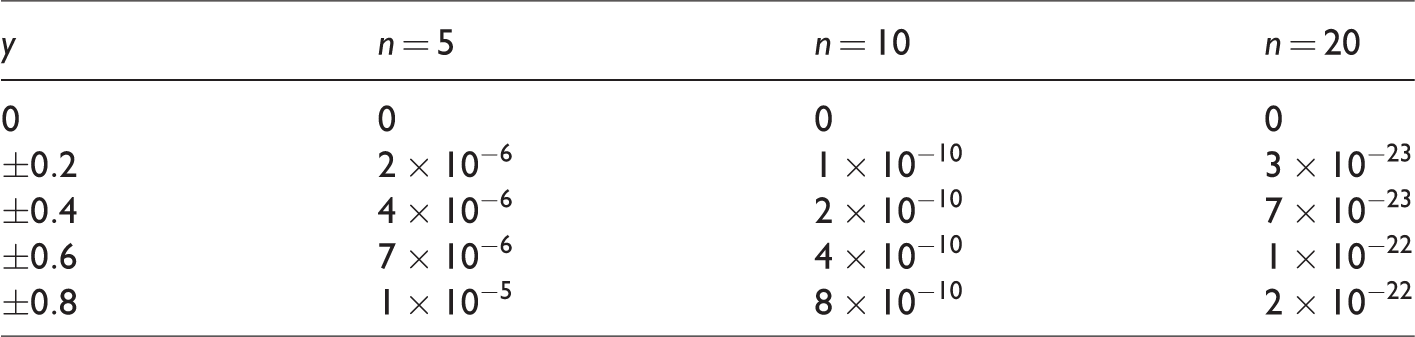
having the proposed procedure, applying equations (3) and (46), the absolute errors of the approximate solution via the MHPM are illustrated in Table 1 for the given y and n. Also, the graph of $u_n(y)$ for different n is to be illustrated in Figure 1.

Figure 1.

Graph of $u_n(y)$ for different n, in Example (5).

Table 1.

Absolute error for different values of n of equation (104).

y	n = 5	n = 10	n = 20
$-0.8$	$1\times {10}^{-4}$	$8\times {10}^{-10}$	$2\times {10}^{-22}$
$-0.6$	$8\times {10}^{-5}$	$4\times {10}^{-9}$	$1\times {10}^{-22}$
$-0.4$	$7\times {10}^{-5}$	$2\times {10}^{-10}$	$6\times {10}^{-22}$
$-0.2$	$6\times {10}^{-5}$	$7\times {10}^{-11}$	$3\times {10}^{-23}$
0	$6\times {10}^{-5}$	$4\times {10}^{-11}$	$7\times {10}^{-24}$
$0.2$	$7\times {10}^{-5}$	$2\times {10}^{-10}$	$4\times {10}^{-23}$
$0.4$	$8\times {10}^{-5}$	$3\times {10}^{-10}$	$8\times {10}^{-23}$
$0.6$	$1\times {10}^{-4}$	$5\times {10}^{-10}$	$1\times {10}^{-22}$
$0.8$	$1\times {10}^{-4}$	$9\times {10}^{-10}$	$3\times {10}^{-22}$

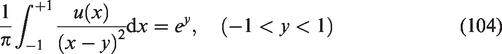
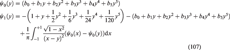
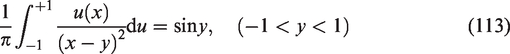
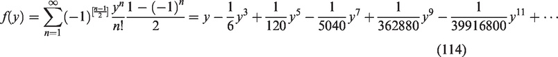
Example 6. The following hypersingular integral equation of the first kind ³³ can be worked out

$$\frac{1}{\pi }{\displaystyle {\int }_{-1}^{+1}\frac{u(x)}{{(x-y)}^2}}\text{d}u=\sin y,(-1<y<1)$$

(113)

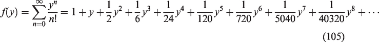
in which $f(y)=\sin y$ expanded using Taylor-polynomial

$$\begin{array}{c}f(y)={\displaystyle \sum _{n=1}^{\infty }{(-1)}^{[\frac{n-1}{2}]}}\frac{y^n}{n!}\frac{1-{(-1)}^n}{2}=y-\frac{1}{6}{y}^3+\frac{1}{120}{y}^5-\frac{1}{5040}{y}^7+\frac{1}{362880}{y}^9-\frac{1}{39916800}{y}^{11}+\cdots \end{array}$$

(114)

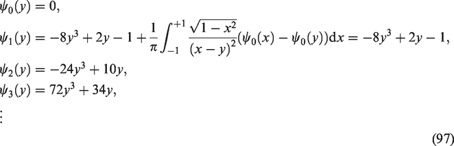
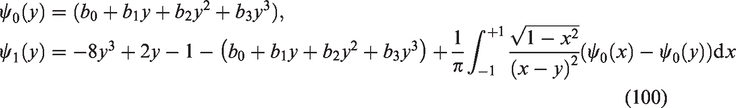
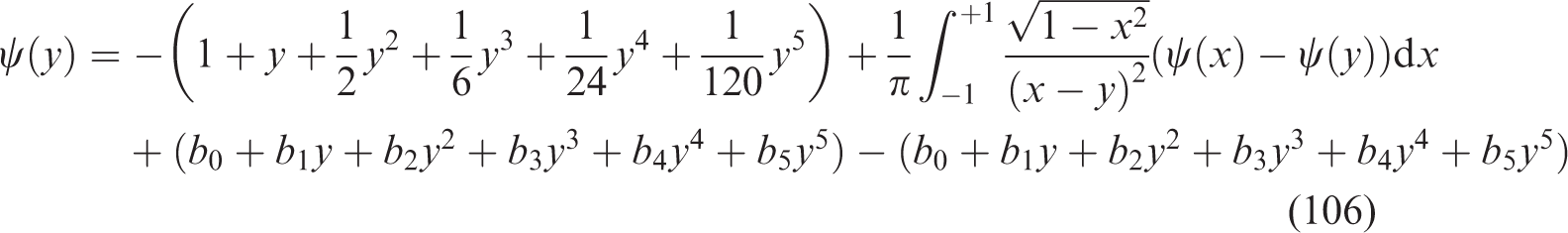
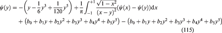
Running the MHPM, using equation (34) for n = 5, the following statement is promised

$$\begin{array}{l}\psi (y)=-\left(y-\frac{1}{6}{y}^3+\frac{1}{120}{y}^5\right)+\frac{1}{\pi }{\displaystyle {\int }_{-1}^{+1}\frac{\sqrt{1-x^2}}{{(x-y)}^2}}(\psi (x)-\psi (y))\text{d}x\\ +\left(b_0+b_{1}y+b_2{y}^2+b_3{y}^3+b_4{y}^4+b_5{y}^5\right)-\left(b_0+b_{1}y+b_2{y}^2+b_3{y}^3+b_4{y}^4+b_5{y}^5\right)\end{array}$$

(115)

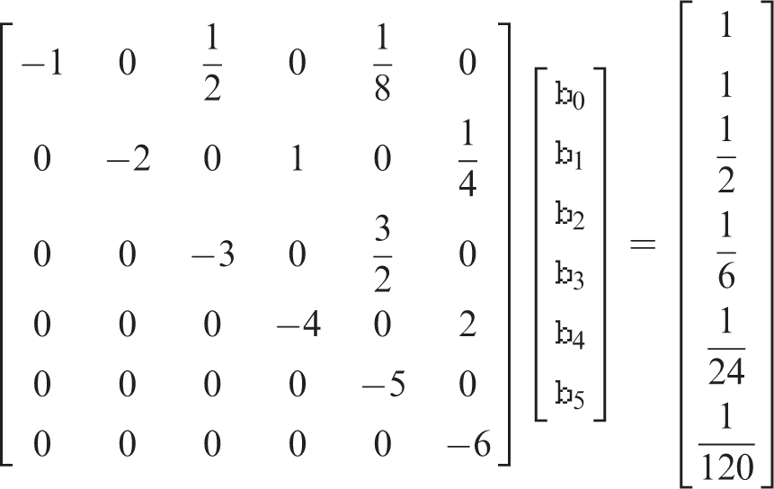
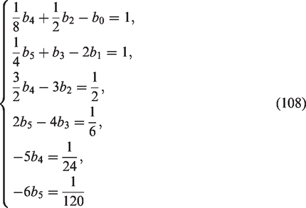
By employing equation (46), it is suitable to announce

$$\begin{array}{l}{\psi }_0(y)=(b_0+b_{1}y+b_2{y}^2+b_3{y}^3+b_4{y}^4+b_5{y}^5)\\ {\psi }_1(y)=-(y-\frac{1}{6}{y}^3+\frac{1}{120}{y}^5)-(b_0+b_{1}y+b_2{y}^2+b_3{y}^3+b_4{y}^4+b_5{y}^5)+\frac{1}{\pi }{\displaystyle {\int }_{-1}^{+1}\frac{\sqrt{1-x^2}}{{(x-y)}^2}}({\psi }_0(x)-{\psi }_0(y))\text{d}x\end{array}$$

(116)

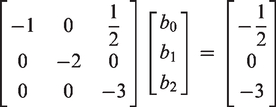
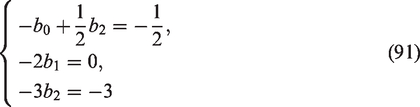
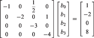
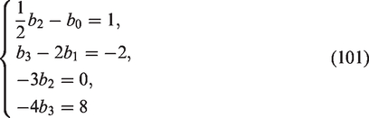
By placing ${\psi }_1(y)=0$ , and according to equation (55), the following system is written

$$\left[\begin{array}{cccccc}-1& 0& \frac{1}{2}& 0& \frac{1}{8}& 0\\ 0& -2& 0& 1& 0& \frac{1}{4}\\ 0& 0& -3& 0& \frac{3}{2}& 0\\ 0& 0& 0& -4& 0& 2\\ 0& 0& 0& 0& -5& 0\\ 0& 0& 0& 0& 0& -6\end{array}\right]\left[\begin{array}{c}{b}_0\\ b_1\\ b_2\\ b_3\\ b_4\\ b_5\end{array}\right]=\left[\begin{array}{c}0\\ 1\\ 0\\ -\frac{1}{6}\\ 0\\ \frac{1}{120}\end{array}\right]$$

Given equation (56), we get

$$\{\begin{array}{l}\frac{1}{8}{b}_4+\frac{1}{2}{b}_2-b_0=0,\hfill \\ \frac{1}{4}{b}_5+b_3-2b_1=1,\hfill \\ \frac{3}{2}{b}_4-3b_2=0,\hfill \\ +2b_5-4b_3=-\frac{1}{6},\hfill \\ -5b_4=0,\hfill \\ -6b_5=\frac{1}{120}\hfill \end{array}$$

(117)

Giving $b_5=-\frac{1}{720},b_4=0,b_3=\frac{59}{1440},b_2=0,b_1=-\frac{307}{640}$ and $b_0=0$ , then

$$\psi (y)={\psi }_0(y)=(-\frac{1}{720}{y}^5+\frac{59}{1440}{y}^3-\frac{307}{640}y)$$

(118)

and next

$$u_5(y)=\left(-\frac{1}{720}{y}^5+\frac{59}{1440}{y}^3-\frac{307}{640}y\right)\sqrt{1-y^2}$$

(119)

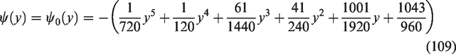
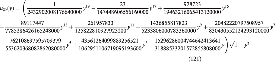
Estimations show that, for n = 10 and n = 20. Now we comprehend the following statements

$$\begin{array}{l}{u}_{10}(y)=(-\frac{1}{3628800}{y}^9+\frac{179}{7257600}{y}^7-\frac{1903}{1382400}{y}^5+\frac{475883}{11612160}{y}^3-\frac{44560951}{92897280}y)\sqrt{1-y^2},\end{array}$$

(120)

$$\begin{array}{l}{u}_{20}(y)=(\frac{1}{2432902008176640000}{y}^{19}-\frac{23}{147448606556160000}{y}^{17}+\frac{928723}{19463216065413120000}{y}^{15}\\ -\frac{89117447}{7785286426165248000}{y}^{13}+\frac{261957833}{125822810927923200}{y}^{11}-\frac{1436855817823}{5233806000783360000}{y}^9+\frac{20482220797508957}{830430552124293120000}{y}^7\\ -\frac{762108697595709379}{553620368082862080000}{y}^5+\frac{43561264099889256521}{1062951106719095193600}{y}^3-\frac{15296286004744642413641}{31888533201572855808000}y)\sqrt{1-y^2}\end{array}$$

(121)

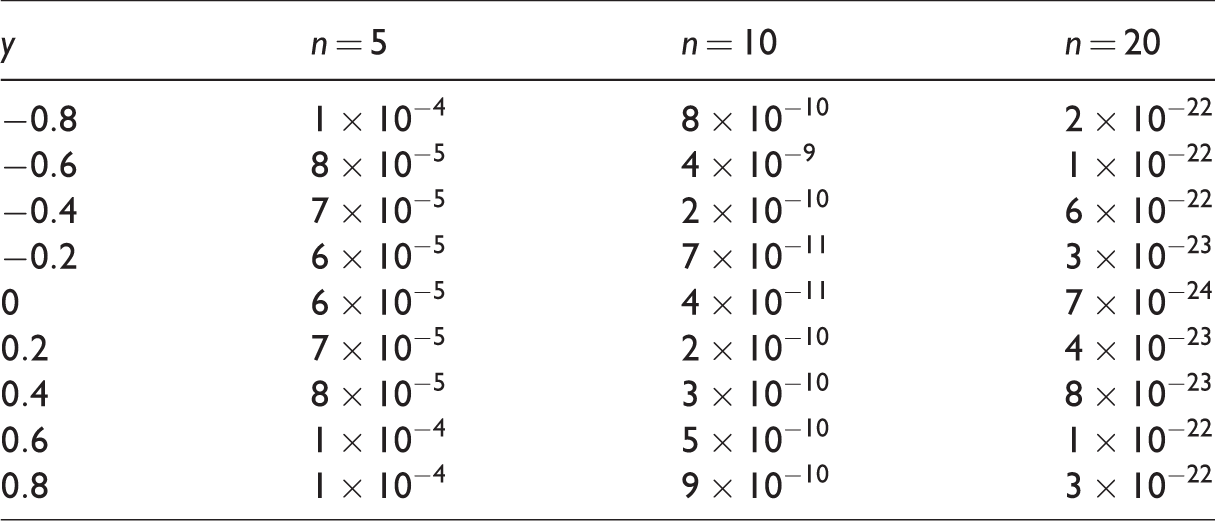
By applying equations (3) and (46), the absolute errors of the approximate solution via the MHPM are illustrated in Table 2 for the given y and n. Also, the graph of $u_n(y)$ for different n is plotted in Figure 2.

Figure 2.

Graph of $u_n(y)$ for different n, in Example (6).

Table 2.

Absolute error for different values of n of equation (113).

y	n = 5	n = 10	n = 20
0	0	0	0
$\pm 0.2$	$2\times {10}^{-6}$	$1\times {10}^{-10}$	$3\times {10}^{-23}$
$\pm 0.4$	$4\times {10}^{-6}$	$2\times {10}^{-10}$	$7\times {10}^{-23}$
$\pm 0.6$	$7\times {10}^{-6}$	$4\times {10}^{-10}$	$1\times {10}^{-22}$
$\pm 0.8$	$1\times {10}^{-5}$	$8\times {10}^{-10}$	$2\times {10}^{-22}$

Conclusion

A vigorous research was provided here to propose a new modified homotopy perturbation method which happened to vacillate achieving solution to a class of hypersingular integral equations of the first kind. Then, the MHPM to which more researchers refer, was discovered to be the most ideal tool in dealing with the complicated function-theoretic analytical structures within an analytical method. Ideally, in this new method, the MHPM, reaching the exact solution can be accomplished where two terms of the series are feasible to be calculated. In addition, results obtained from considerable examples report a high degree of validity and accuracy of the MHPM.