In this work, the variational iteration algorithm-I with an auxiliary parameter is used for the analytical treatment of the wave equations and wave-like vibration equations. The technique has the capability of reducing the size of computational work and easily overcomes the difficulty of the perturbation method or Adomian polynomials. Comparison with the classic variational iteration algorithm-I (VIA-1) is carried out, showing that the modification is more efficient and reliable.
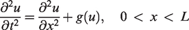
In recent years, wave-like equations, linear and nonlinear wave equations have much been attracted by many scientists and researchers, which arises in different fields of sciences and engineering, i.e. physics, fluid dynamics, electromagnetics, and acoustics. Many verities in sciences and engineering can be explained by nonlinear partial differential equations. It is still difficult to find out the analytical or numerical solution which exists in real life nonlinear models. Consider the following wave equations
and
where g(u) is a linear function. The vibrational behavior of beams and shafts can be expressed in terms of waves.1 The motion of the system of vibrating beams, rods, and springs reduces to that of the wave equation. The wave equation is probably the most used partial differential equation (PDE) in practical applications. Waves exist in different media like as in geophysics there are surface and internal waves in the ocean, but there are also more complex nonlinear models comparing to PDE. There are wave processes in the Earth (seismic waves), acoustic waves in the air and water, electromagnetic waves in different media. Initial equations differ for each case, but the wave equation can be derived in some approximation in most of the cases.
The aim of this work is to apply the VIA-I with an auxiliary parameter (AP) for the analytical treatment of the wave equations. The VIA-I with an AP is the modified form of VIA-I,2 which was developed by a Chinese mathematician He,3,4 in 1999. He5 himself advanced the method to a great extent. Hesameddini and Latifizadeh6 constructed an idea of variational iteration algorithm based on Laplace transformation. Salkuyeh7 showed the convergence of the variational iteration algorithm for solving linear system of ordinary differential equation with variable coefficients. Fractional calculus,8 inverse problems,9 differential-difference equations,10 and an integro-differential equations11,12 all these need the application of this method for effective solutions. The system of boundary value problems of higher order can also be solved by this algorithm proved by Noor and Mohyud-Din.13
From time to time, modifications have been brought into the variational iteration algorithm. One of those modifications, Herisanu and Marincaut modification14 is quite attractive. In this modification, this algorithm has been linked with the least squares technology. To improve the convergence speed and effectiveness of this algorithm, Noor and Mohyud-Din15,16 has modified it by coupling it with the generalized Taylor series. Later, Hosseini et al.17 presented an appropriate procedure for finding the optimal value of AP. This method is recently further modified for vector functions by introducing matrix Lagrange multiplier.18,19
The main characteristic of this method is the presence of the elements of flexibility and ability in solving nonlinear and linear problems. This method is independent of the complexities of Adomianit polynomials. There is no need of concretization, linearization, or unrealistic assumptions. One of the main characteristics of this technique is that approximate solution of great correctness can be obtained by only a few iterations. This method has a simple procedure, acceptable results and above all, it can be practically used for a greater number of nonlinear problems.20–30
Variational iteration algorithm-I
Consider the following nonlinear differential equation
where “L” is the linear operator, “N” being the non-linear operator, and “c(x)” is the inhomogeneous source term. Constructing a correction function
where “ λ” is the parameter, which is not known and called the Lagrange multiplier. Now, taking the δ on the one side as well as the other side of equation (2) with respect to
where is known as restricted term which applies that
Since the Lagrange multiplier λ is a basic and of great importance in the method as it may be a constant or a function. Therefore, first we will find out the λ, which can be found using integration by parts easily, furthermore by the successive approximation upon for the solution of , will be obtained without any difficulty by using the obtained values of λ and by using an initial approximation with possible unknowns. As a result, the exact solution of the given equation can be obtained by utilizing
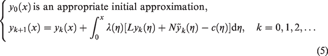
In summary, the variational iteration algorithm-I is given as
The above technique of finding the approximate solution is called VIA-I, which is the advancement of the general Lagrange multiplier strategy proposed by Inokuti et al.31 Now this method4,32,33 has been produced to solve a considerable measure of nonlinear problems emerge in various fields of sciences.
VIA-I with an AP
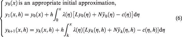
In VIA-I, introducing an unknown AP represented by h, which was used in homotopy perturbation method34–37 before, enhances the effectiveness and exactness of the technique. Presenting h in equation (5)
Here, has an unknown AP h, which makes sure the convergence to the exact solution. This procedure is known as VIA-I with an AP. Actually, this technique is simple, has a lesser size of calculation, not difficult to analyze, and have the ability to approximate the solution exactly in the solution domain of wide range. For the convergence of this technique, see Ghaneai and Hosseini.38
Convergence analysis
The convergence of our proposed modification, called VIA-I with an AP when applied to equation (1), is studied in this section. When this proposed technique is applied to wave equations and wave-like vibration equations, L, which is a linear operator, it can be defined as and . Now, defining the operator B as below
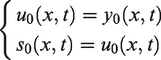
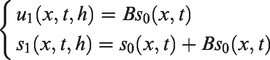
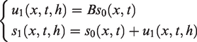
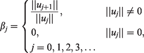
and defining the components , and 0 as below
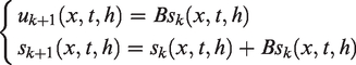
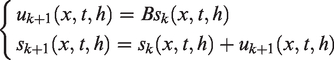
Generally, we can write it for
as a result
The can be uninhibitedly picked if the given initial and boundary conditions are satisfied by it. If a proper initial approximation is chosen, the method will give accurate and fruitful results successfully. We can approximate the solution by kth-order truncated series as This has an AP, which make sure that with the help of norm 2 error of the residual function, the assumption can be satisfied. Error estimate and adequate conditions for convergence of VIA-I with an AP are explained. The main results are proposed in the accompanying theorems.39,40
Theorem 1
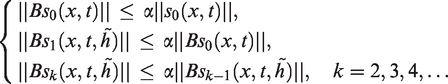
Let H be a Hilbert space and B, defined in equation (7), be an operator from a Hilbert space H to H. The series solution (8)
converges if such that,
Proof
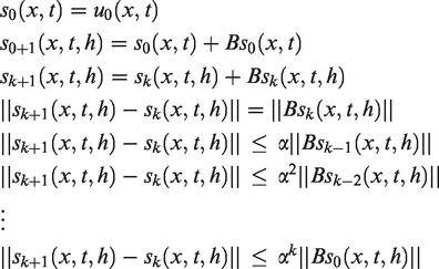
We have to show that the sequence is a Cauchy sequence in the Hilbert space H.
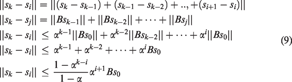
For this purpose, consider
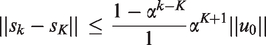
for , , Thus
For every
and since
we obtain
Hence, it is proved that the sequence is a Cauchy sequence in the Hilbert space H which implies that converges.
Theorem 2
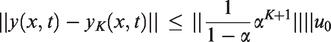
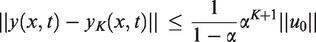
Assume that the series solution (8) converges to exact solution of equation (1). If the truncated series supposed to be the approximate solution, then the max error can be estimated as
Proof
From Theorem 1
since we obtain
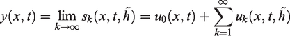
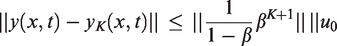
This finishes the proof. In short, we can define
here, if of equation (1) converges to an exact solution . While the maximum absolute error
Solving this wave equation by VIA-I, we have to form the rectification function for it, which is
Lagrange multiplierio value can be found out by the use of variational theory, which is
The following iterative scheme can be obtained by the use of value in equation (12)
initializing with .
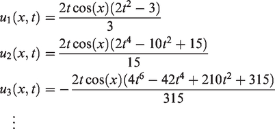
With the help of this iterative scheme (13), other approximations can be obtained
we finish the process at .
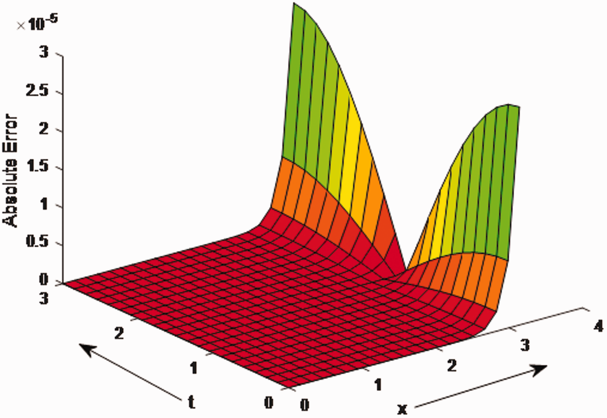
The absolute error of in the solution domain is shown in Figure 1.
Absolute error betwixt the exact solution and numerical solution by VIA-I.
In Figure 1, it is obvious that VIA-I diverges for higher values of .
Now solving by VIA-I with AP, the recurrence relation for equation (10) is
initializing with .
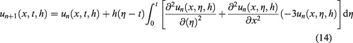
With the help of this recurrence relation (14), other approximations can be obtained
we finish the process at .
For the estimation of AP , the residual function
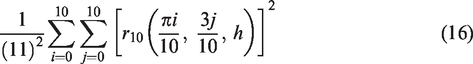
The square of equation (15) for 10th-order approximation with respect to is
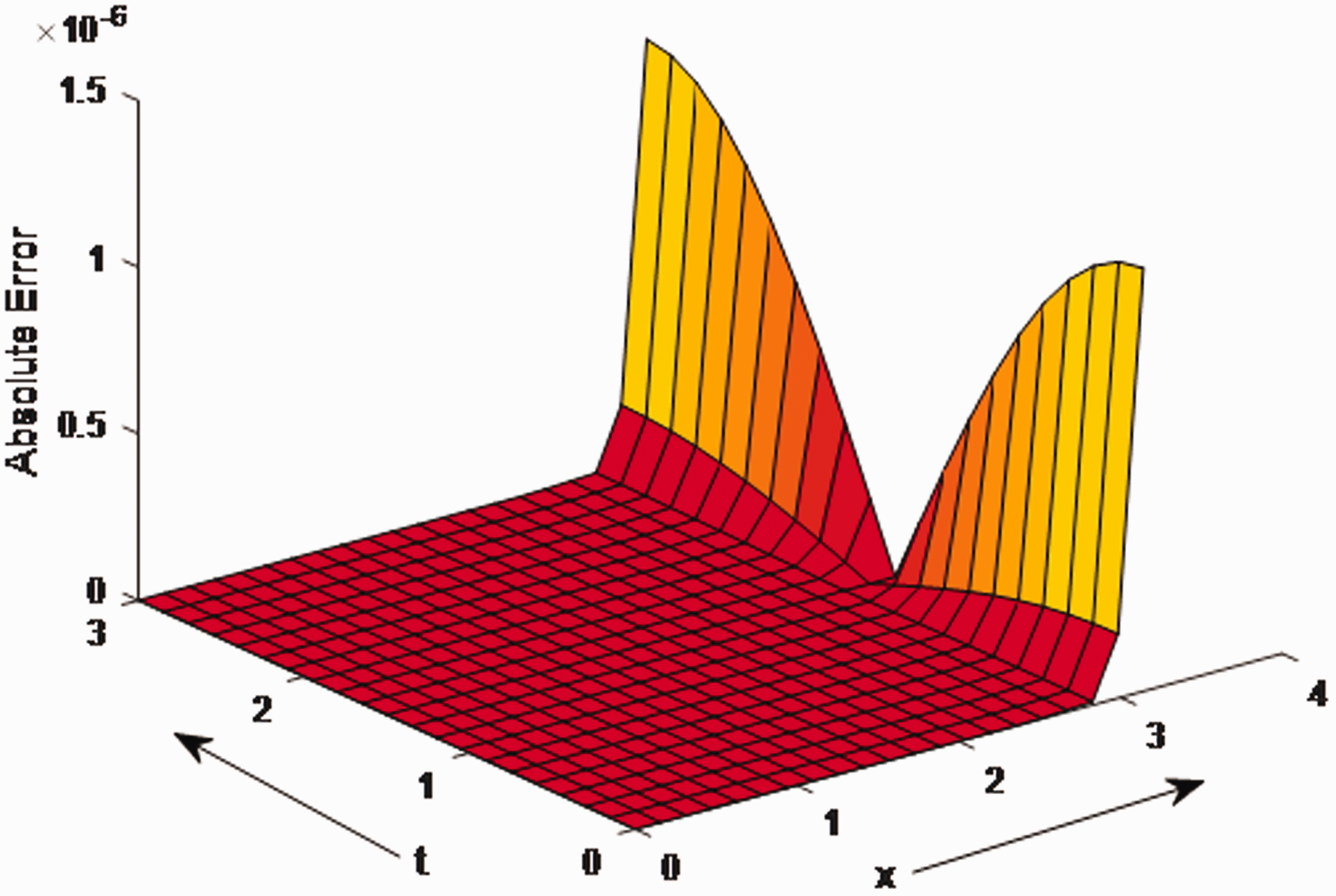
The minimum value of equation (16) happens at . Utilizing this estimation of in the solution domain , the absolute error betwixt the exact and numerical solutions can be seen in Figure 2.
Absolute error betwixt the exact solution and numerical solution by VIA-I with AP.
Comparing Figures 1 and 2, it is clear that VIA-I with AP gives better results as compared to VIA-I.
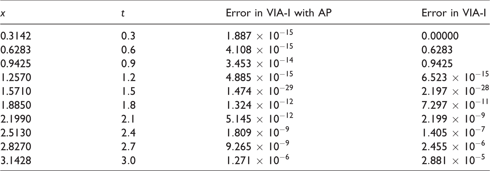
Numerical comparison betwixt the exact and numerical solutions of both methods is given in Table 1, which shows that VIA-I with AP is better for a large domain of t as compared to VIA-I.
Comparison of absolute errors for 10th-order approximation by VIA-I and VIA-I with AP.
Error in VIA-I with AP
Error in VIA-I
0.3142
0.6283
0.9425
1.2570
1.5710
1.8850
2.1990
2.5130
2.8270
3.1428
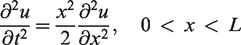
The wave-like vibration equation
Consider the following wave-like vibration equation41
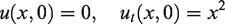
subjected to the initial conditions
and the exact solution
Solving this wave equation by VIA-I, we have to form the rectification function for it, which is
Lagrange multiplierio value can be found out by the use of variational theory, which is
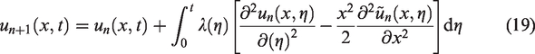
The following iterative scheme can be obtained by the use of value in equation (19)
initializing with .
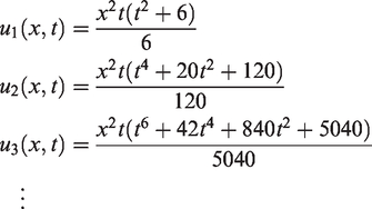
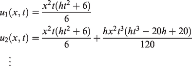
With the help of this iterative scheme (20), other approximations can be obtained
we finish the process at .
The absolute error of in the solution domain can be seen in Figure 3.
Absolute error betwixt the exact solution and numerical solution by VIA-I.
In Figure 3, it is obvious that VIA-I diverges for higher values of .
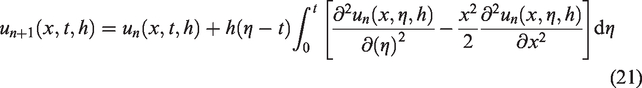
Now solving by VIA-I with AP, the recurrence relation for equation (17) is
starting with .
With the help of this iterative scheme (21), other approximations can be obtained
we finish the procedure at .
For the estimation of AP , the residual function
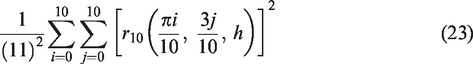
The square of equation (22) for 10th-order approximation with respect to is
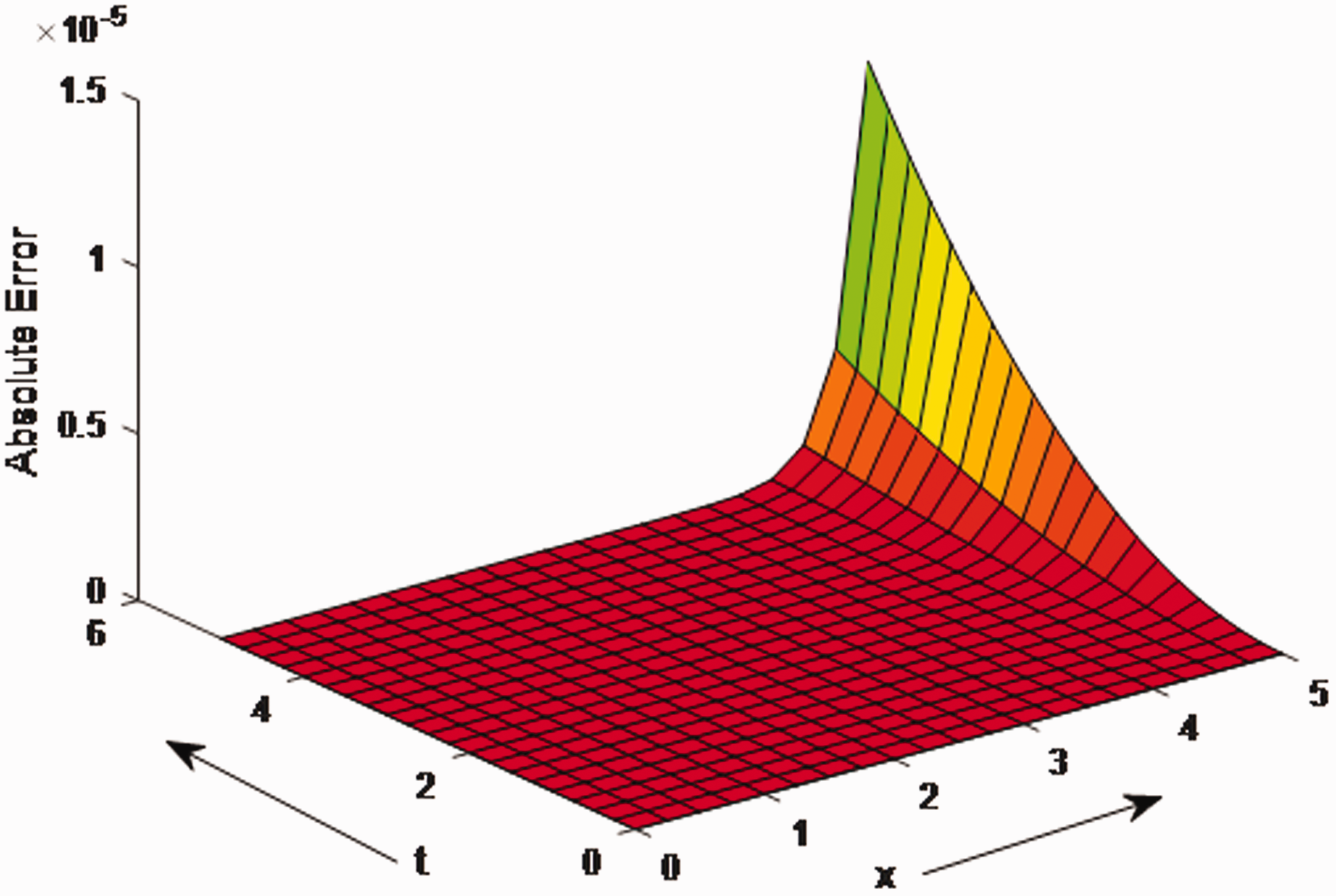
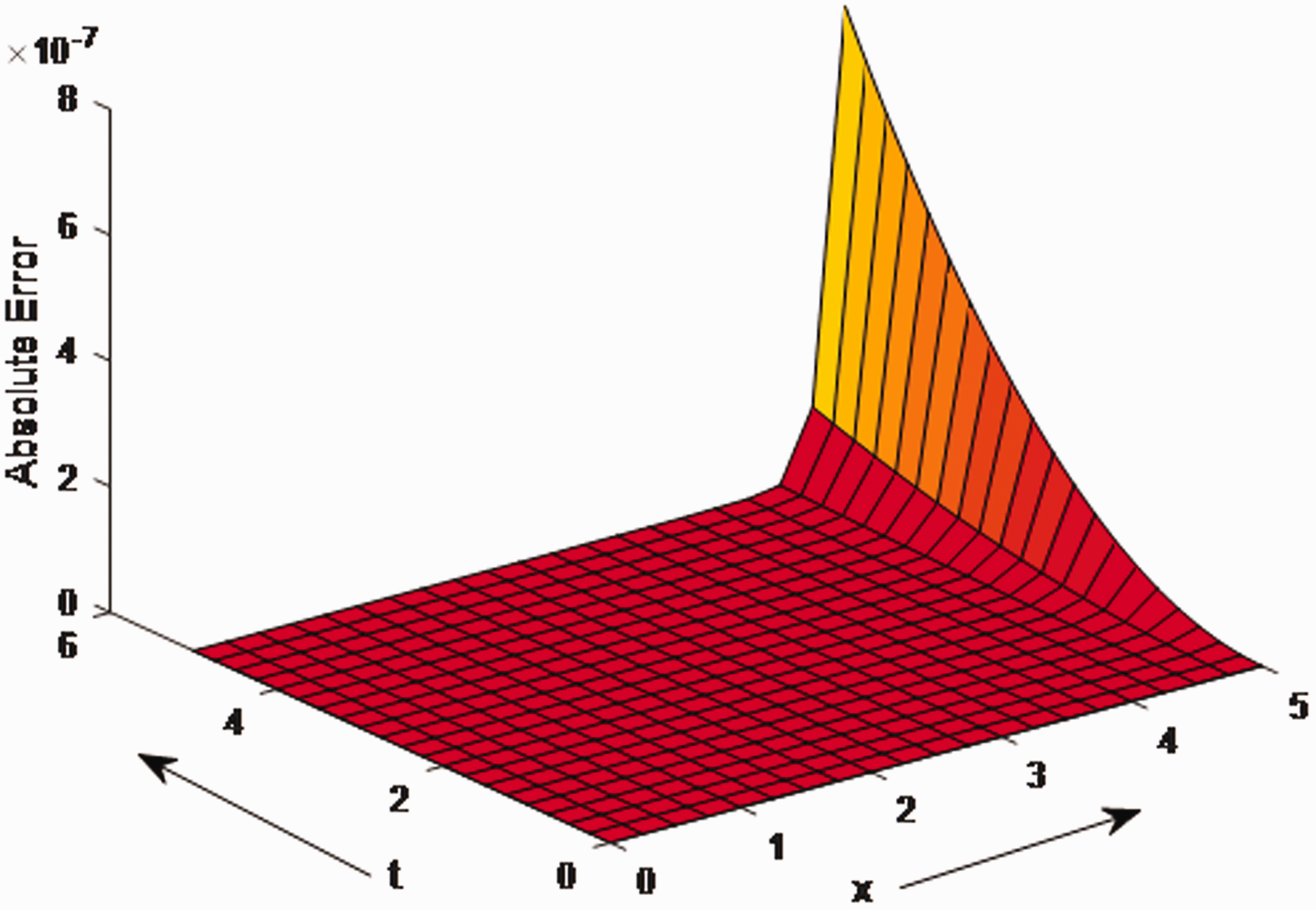
The minimum value of equation (23) happens at . Utilizing this estimation of in the solution domain , the absolute error can be found in Figure 4.
Absolute error betwixt the exact solution and numerical solution by VIA-I with AP.
Comparing Figures 3 and 4, it is clear that VIA-I with AP gives better results as compared to VIA-I. Numerical comparison between the exact and numerical solutions of both methods is given in Table 2.
Comparison of absolute errors for 10th-order approximation by VIA-I and VIA-I with AP.
Error in VIA-I with AP
Error in VIA-I
0.5
1.0
1.5
2.0
2.5
3.0
3.5
4.0
4.5
5.0
It is clear from the numerical results that VIA-I with AP is better for a large domain of as compared to VIA-I.
Conclusion
In this paper, we presented a modified version of VIA-I for handling wave equations. VIA-I with an AP worked to give accurate solutions to these wave equations in a successful manner. The technique converges very quickly and deals with linear and nonlinear problems in an efficient way. In this technique, there is no need to take any integration or convolution theorem in recurrence relation to find out the Lagrange multipliers. Discretization, linearization, and small parameter assumptions are not required, which actually ruins the physical nature of the problem. It can be easily seen that VIA-I with an AP is a reliable, efficient, powerful, and fast convergent method. There is no particular need to deal with nonlinear terms. Nonlinear models are as often as possible emerging in physical science and engineering problems for communicating nonlinear marvels. VIA-I with an AP provides a reliable and promising method for dealing with this nonlinear behavior and is more efficient and accurate as compared to classic VIA-I.
Footnotes
Declaration of conflicting interests
The author(s) declared no potential conflicts of interest with respect to the research, authorship, and/or publication of this article.
Funding
The author(s) received no financial support for the research, authorship, and/or publication of this article.
References
1.
MaceB.Wave reflection and transmission in beams. J Sound Vib1984;
97: 237–246.
2.
HeJHWuGCAustinF.The variational iteration method which should be followed. Nonlinear Sci Lett A2010;
1: 1–30.
3.
HeJH.Variational iteration method – a kind of non-linear analytical technique: some examples. Int J Non-Linear Mech1999;
34: 699–708.
4.
HeJH.Variational iteration method some recent results and new interpretations. J Comput Appl Math2007;
207: 3–17.
5.
HeJH.Some asymptotic methods for strongly nonlinear equations. Int J Mod Phys B2006;
20: 1141–1199.
6.
HesameddiniELatifizadehH.Reconstruction of variational iteration algorithms using the Laplace transform. Int J Nonlinear Sci Numer Simul2009;
10: 1377–1382.
7.
SalkuyehDK.Convergence of the variational iteration method for solving linear systems of odes with constant coefficients. Comput Math Appl2008;
56: 2027–2033.
8.
AteşİYildirimA.Application of variational iteration method to fractional initial-value problems. Int J Nonlinear Sci Numer Simul2009;
10: 877–884.
9.
ChunC.Variational iteration method for a reliable treatment of heat equations with ill-defined initial data. Int J Nonlinear Sci Numer Simul2008;
9: 435–440.
10.
MokhtariR.Variational iteration method for solving nonlinear differential-difference equations. Int J Nonlinear Sci Numer Simul2008;
9: 19–24.
11.
Saberi-NadjafiJTamamgarM.The variational iteration method: a highly promising method for solving the system of integro-differential equations. Comput Math Appl2008;
56: 346–351.
12.
MomaniSNoorMA.Numerical methods for fourth-order fractional integro-differential equations. Appl Math Comput2006;
182: 754–760.
13.
NoorMAMohyud-DinST.Variational iteration technique for solving higher order boundary value problems. Appl Math Comput2007;
189: 1929–1942.
14.
HerisanuNMarincaV.A modified variational iteration method for strongly nonlinear problems. Nonlinear Sci Lett A2010;
1: 183–192.
15.
NoorMAMohyud-DinST.Modified variational iteration method for solving fourth-order boundary value problems. J Appl Math Comput2009;
29: 81–94.
16.
NoorMAMohyud-DinST.Variational iteration method for solving higher-order nonlinear boundary value problems using Heiteration meth. Int J Nonlinear Sci Numer Simul2008;
9: 141–156.
17.
HosseiniMMohyud-DinSTGhaneaiH, et al.
Auxiliary parameter in the variational iteration method and its optimal determination. Int J Nonlinear Sci Numer Simul2010;
11: 495–502.
18.
HeWKongHQinYM.Modified variational iteration method for analytical solutions of nonlinear oscillators.J Low Freq Noise Vibr Act Control2018. DOI: 10.1177/1461348418784817
19.
ChengHYuYY.Semi-analytical solutions of the nonlinear oscillator with a matrix Lagrange multiplier.J Low Freq Noise Vibr Act Control2018.
20.
BiazarJGholaminPHosseiniK.Variational iteration method for solving FokkeraPlanck equation. J Franklin Inst2010;
347: 1137–1147.
21.
El-SayedTEl-MongyH.Application of variational iteration method to free vibration analysis of a tapered beam mounted on two-degree of freedom subsystems. Appl Math Modell2018;
58: 349–364.
22.
RafiqMAhmadHMohyud-DinST.Variational iteration method with an auxiliary parameter for solving volterras population model. Nonlinear Sci Lett A2017;
8: 389–396.
23.
HeJHWuXH.Construction of solitary solution and compacton-like solution by variational iteration method. Chaos Solitons Fractals2006;
29: 108–113.
24.
AhmadH.Variational iteration method with an auxiliary parameter for solving differential equations of the fifth order. Nonlinear Sci Lett A2018;
9: 27–35.
25.
OdibatZMomaniS.Application of variational iteration method to nonlinear differential equations of fractional order. Int J Nonlinear Sci Numer Simul2006;
7: 27–34.
26.
HeJH.Variational iteration method for autonomous ordinary differential systems. Appl Math Comput2000;
114: 115–123.
27.
AbdouMSolimanA.New applications of variational iteration method. Phys D2005;
211: 1–8.
28.
AbbasbandyS.A new application of He nevariational iteration method for quadratic Riccati differential equation by using Adomian’s polynomials. J Comput Appl Math2007;
207: 59–63.
29.
GanjiDSadighiA.Application of homotopy-perturbation and variational iteration methods to nonlinear heat transfer and porous media equations. J Comput Appl Math2007;
207: 24–34.
30.
Wu GC and LeeE.Fractional variational iteration method and its application. Phys Lett A2010;
374: 2506–2509.
31.
InokutiMSekineHMuraT.General use of the Lagrange multiplier in nonlinear mathematical physics. Variational Method Mech Solids1978;
33: 156–162.
32.
HeJH.Variational approach to the ThomasoFermi equation. Appl Math Comput2003;
143: 533–535.
33.
AhmadH.Auxiliary parameter in the variational iteration algorithm-ii and its optimal determination. Nonlinear Sci Lett A2018;
9: 62–72.
34.
WuYHeJH.Homotopy perturbation method for nonlinear oscillators with coordinate-dependent mass. Results Phys2018;
10: 270–271.
35.
HeJH.Homotopy perturbation method with two expanding parameters. Indian J Phys2014;
88: 193–196.
36.
YuDNHeJHGarcaAG.Homotopy perturbation method with an auxiliary parameter for nonlinear oscillators. J Low Freq Noise Vibr Act Control2018. DOI: 10.1177/1461348418811028
37.
LiXXHeCH.Homotopy perturbation method coupled with the enhanced perturbation method. J Low Freq Noise Vibr Act Control2018. DOI: 10.1177/1461348418800554
38.
GhaneaiHHosseiniM.Variational iteration method with an auxiliary parameter for solving wave-like and heat-like equations in large domains. Comput Math Appl2015;
69: 363–373.
39.
OdibatZM.A study on the convergence of variational iteration method. Math Comput Model2010;
51: 1181–1192.
40.
GhaneaiHHosseiniM.Solving differential-algebraic equations through variational iteration method with an auxiliary parameter. Appl Math Model2016;
40: 3991–4001.
41.
WazwazAM.The variational iteration method: a reliable analytic tool for solving linear and nonlinear wave equations. Comput Math Appl2007;
54: 926–932.