The spring load adjustment method for six-axle high-power locomotives

Abstract

The stability and comfort of locomotives need to be guaranteed by load adjustment technology. Considering the defects of the traditional two-step adjustment method for locomotive load distribution, including its lack of efficiency and error accumulation, a new technical approach is developed here under entire locomotive conditions, simulating the load adjustment test via the application of shimming under the treads. In the case of high-power locomotives, a complete theoretical model is established based on the classical two-suspension model. According to the difference between shimming on the treads and on primary suspension positions, a transformation matrix is established with which to describe the conversion relationship between the shim quantity on the primary supporting positions and on the treads. Considering that locomotive load regulation is a nonlinear problem characterised by nonlinearity, parametric uncertainty and multiple optimisation objectives, this paper proposes QAGA, an optimisation algorithm for entire locomotive load adjustment based on an adaptive genetic algorithm and a quantum-behaved particle swarm optimisation algorithm, to carry out simulations using data from an HXD1D-type electric locomotive. Analysis of the simulation results proves that the proposed approach can significantly improve the efficiency, accuracy and feasibility of the entire locomotive load adjustment process.

Introduction

The load distribution of locomotive wheels (axles) significantly influences the dynamic, traction, braking and adhesive performance of high-power locomotives. Thus, research on load adjustment technology is of significant practical importance.^1–3 A large wheel (axle) load deviation can not only cause wheel idling or sliding, but can also lead to axle vibration at high frequencies, resulting in the deterioration of locomotive traction and braking performance. ⁴ Therefore, a shimming operation is added to the locomotive debugging process to reduce the static load deviation.

Related researches have been done by European scholars since early times to guide the shimming operation. A mathematical model has been built by Nenov et al. ⁵ and algorithm and software have been developed based on it to determine the necessary corrections of the supporting planes of spring elements. And the German Windhoff AG company has developed the bogie load test bench for locomotive primary spring adjustment by cooperating with China locomotive manufacturing giant CRRC. ⁶ In China, many methods are proposed for the optimisation of the static load distribution of locomotives. These algorithms can be divided into the following three categories: (1) The spring adjustment method based on iterative operation, (2) the spring adjustment algorithms using ideas of evolutionary and particle swarm optimisation^7–9 and (3) the multi-objective spring adjustment strategy. ¹⁰ The researches above have been proved to be helpful via tests on real locomotives.

However, there is still room and need for further improving the load adjusting method to meet the demand of practical application.

First, nowadays the most common approach is to adjust the locomotive load distribution on primary^11,12 and secondary^13–15 suspension positions separately. However, such two-step adjustment methods cannot avoid problems of low efficiency, high cost and complex operation. Therefore, the present paper introduces a new technical approach that involves adjusting the whole locomotive (including the locomotive body and bogie) load distribution by shimming on treads under entire locomotive conditions.

Second, the load adjustment of a locomotive wheel (axle) is characterised by nonlinearity, parametric uncertainty and multiple optimisation objectives. This process includes the optimisation process of the shim quantity, number of shimming positions, maximum load difference and load variance. It also requires an algorithm offering both high efficiency and precision. So we propose QAGA, an optimisation algorithm for entire locomotive load adjustment based on the quantum-behaved particle swarm optimisation (QPSO) algorithm and the adaptive genetic algorithm (AGA).

The main contributions of this paper are as follows:

In the past, the body load and bogie load of locomotives were adjusted separately in the process of load adjustment in the major locomotive factories in the world. Therefore, the whole adjustment process is divided into two independent steps.^9–13 However, the two-step adjustment process suffers from drawbacks of low efficiency, error accumulation and high cost. To get rid of the defects of the traditional two-step adjustment method for locomotive load distribution, the one-step load adjustment method is proposed in this paper. This new technical approach simulates the primary shimming process by lifting the tread. The advantage of the method is that it can establish the measured model and is easy to verify.

Taking a six-axle high-power locomotive as an example, this paper extends the complete locomotive statics theoretical model from the secondary system to the wheelset on the basis of the existing classical two-system model.

Referring to the method of establishing the measured model in the car body load adjustment, a method of establishing the measured tread model for the whole wheel axle load adjustment is proposed.

The conversion model between the wheel load and primary spring load is established to reveal how the wheel load changes with shimming.

With the help of a simplified model of the primary suspension structure, a comparison is made between the tread lifting and the primary shimming process, and the conversion relationship between the tread lifting and the primary shimming process is obtained, and the influence matrix of the tread lifting on the whole wheel weight is established.

Research on the entire locomotive model

Two-suspension model of a six-axle locomotive

Considering the large size of the locomotive, high technology level and little difference in production size, the simplification of the static model of the vehicle is based on the following basic assumptions for convenience of analysis:

Suppose that the locomotive’s centre of gravity is concentrated at a point, which is located at the centre of gravity of the plane of the chassis.

Assuming that the locomotive is symmetrical in structure, its centroid is located at the intersection of the longitudinal and transverse symmetrical planes of the locomotive.

The contact surfaces between the secondary spring and the bogie, the primary spring and the bogie, and the contact surfaces between the wheel and the track are simplified as contact points.

Figure 1 shows the actual scene of the locomotive load adjustment experiment. Figure 2 shows the model of a six-axle locomotive with a two-suspension structure, including 12 secondary suspension positions numbered from 1 to 12 and 12 primary suspension positions numbered from 13 to 24. Figure 2 shows the three-dimensional model and the two dimensional simplified model. Figures 3 and 4 display force analysis diagrams of the front and rear bogies, respectively.

Figure 1.

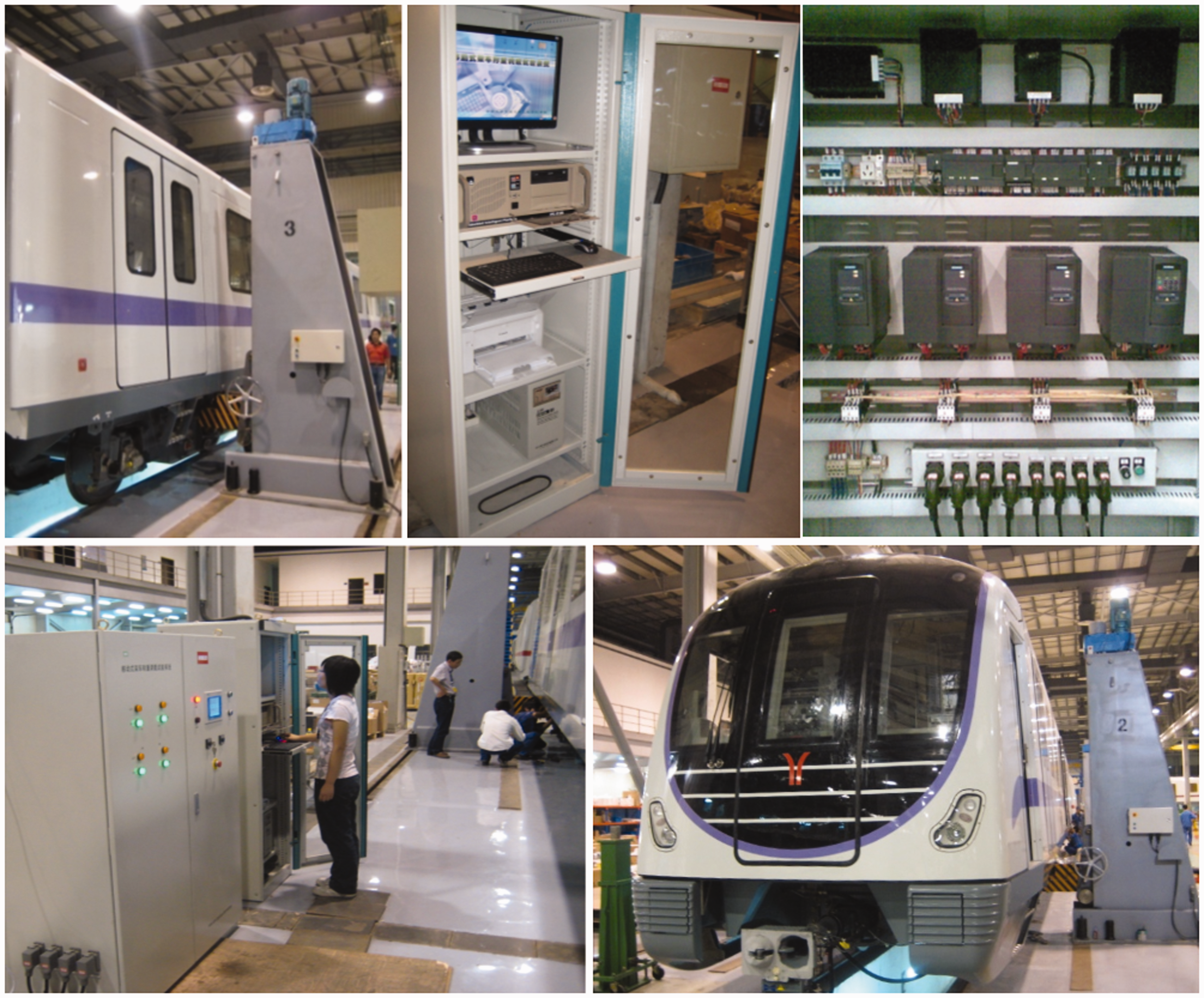
The scene of the locomotive load adjustment experiment.

Figure 2.

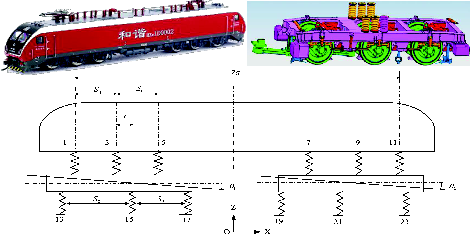
Two-suspension model.

Figure 3.

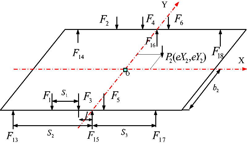
Force analysis of the front bogie.

Figure 4.

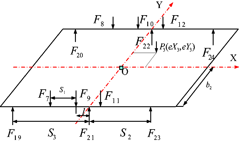
Force analysis of the rear bogie.

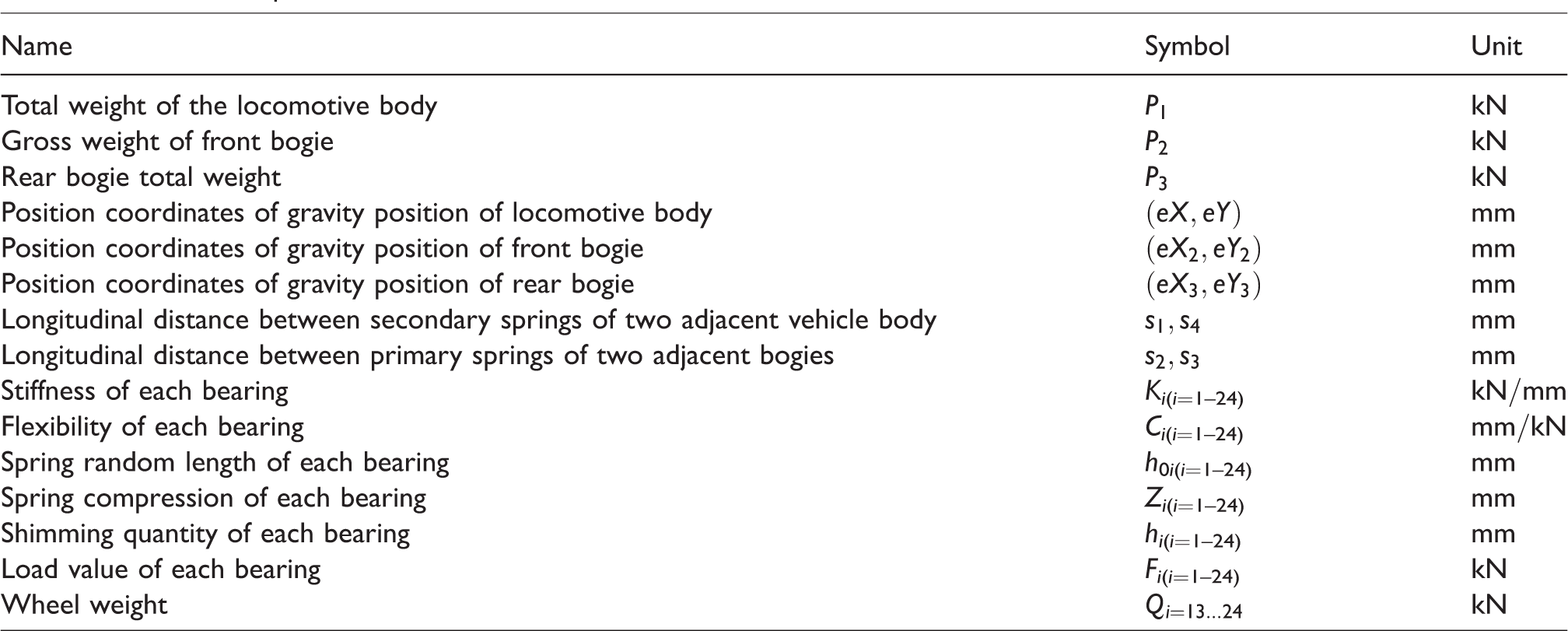
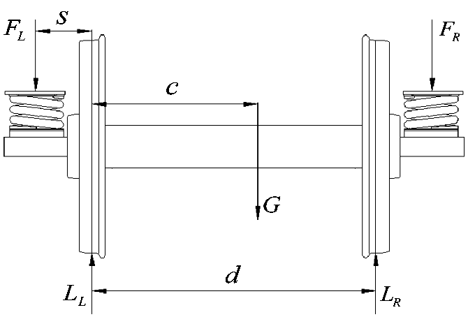
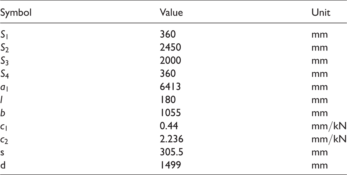
The definition of the main parameters in this paper is shown in Table 1.

Table 1.

List of main parameters in this article.

Name	Symbol	Unit
Total weight of the locomotive body	$P_{\text{1}}$	$\text{kN}$
Gross weight of front bogie	$P_2$	$\text{kN}$
Rear bogie total weight	$P_{\text{3}}$	$\text{kN}$
Position coordinates of gravity position of locomotive body	$\left(eX,eY\right)$	$\text{mm}$
Position coordinates of gravity position of front bogie	$(e{X}_2,e{Y}_2)$	$\text{mm}$
Position coordinates of gravity position of rear bogie	$\left(e{X}_3,e{Y}_3\right)$	$\text{mm}$
Longitudinal distance between secondary springs of two adjacent vehicle body	$s_1,s_4$	$\text{mm}$
Longitudinal distance between primary springs of two adjacent bogies	$s_2,s_3$	$\text{mm}$
Stiffness of each bearing	Ki ( i =1–24)	$\text{kN/mm}$
Flexibility of each bearing	Ci ( i =1–24)	$\text{mm/kN}$
Spring random length of each bearing	h 0 i ( i =1–24)	$\text{mm}$
Spring compression of each bearing	Zi ( i =1–24)	$\text{mm}$
Shimming quantity of each bearing	hi ( i =1–24)	$\text{mm}$
Load value of each bearing	Fi ( i =1–24)	$\text{kN}$
Wheel weight	${\hspace{0.17em}}_Q{\hspace{0.17em}}_{i=\mathrm{13\dots 24}}$	$\text{kN}$

The statics equations of the locomotive body are established as follows

$$\begin{array}{l}{{\displaystyle \sum DF}}_i=0\Rightarrow \Delta F_1+\Delta F_2+\Delta F_3+\Delta F_4+\Delta F_5+\Delta F_6\\ +\Delta F_7+\Delta F_8+\Delta F_9+\Delta F_{10}+\Delta F_{11}+\Delta F_{12}=0\end{array}$$

(1)

$$\begin{array}{l}\sum \Delta M_x=P_1\Delta e{X}_1\Rightarrow P_1\Delta e{X}_1=a_1\Delta F_1+a_1\Delta F_2+(a_1-S_4)\Delta F_3\\ +(a_1-S_4)\Delta F_4+(a_1-S_1-S_4)\Delta F_5+(a_1-S_1-S_4)\Delta F_6\end{array}$$

(2)

$$\begin{array}{l}\sum \Delta M_y=P_1\Delta e{Y}_1\Rightarrow P_1\Delta e{Y}_1=(\Delta F_1-\Delta F_2+\Delta F_3-\Delta F_4\\ +\Delta F_5-\Delta F_6+\Delta F_7-\Delta F_8+\Delta F_9-\Delta F_{10}+\Delta F_{11}-\Delta F_{12})b_1\end{array}$$

(3)

The statics equations of the front bogie

$$\begin{array}{c}{\displaystyle \sum \Delta F}=0\Rightarrow \Delta F_1+\Delta F_2+\Delta F_3+\Delta F_4+\Delta F_5+\Delta F_6\\ =\Delta F_{13}+\Delta F_{14}+\Delta F_{15}+\Delta F_{16}+\Delta F_{17}+\Delta F_{18}\end{array}$$

(4)

$$\begin{array}{l}\sum \Delta M_x=P_2\Delta e{X}_2\Rightarrow P_2\Delta e{X}_2=(\Delta F_1+\Delta F_2)(S_4+l)+(\Delta F_3+\Delta F_4)l\\ -(\Delta F_5+\Delta F_6)(S_1-l)-S_2(\Delta F_{13}+\Delta F_{14})+S_3(\Delta F_{17}+\Delta F_{18})\end{array}$$

(5)

$$\begin{array}{l}{\displaystyle \sum \Delta M_y=}{P}_2\Delta e{Y}_2\Rightarrow P_2\Delta e{Y}_2=(\Delta F_1-\Delta F_2+\Delta F_3-\Delta F_4+\Delta F_5\\ -\Delta F_6)b_1-(\Delta F_{13}-\Delta F_{14}+\Delta F_{15}-\Delta F_{16}+\Delta F_{17}-\Delta F_{18})b_2\end{array}$$

(6)

The statics equations of the rear bogie

$$\begin{array}{l}{\displaystyle \sum \Delta F=0\Rightarrow \Delta F_{19}+\Delta F_{20}+\Delta F_{21}+\Delta F_{22}+\Delta F_{23}+\Delta F_{24}}\\ =\Delta F_7+\Delta F_8+\Delta F_9+\Delta F_{10}+\Delta F_{11}+\Delta F_{12}\end{array}$$

(7)

$$\begin{array}{l}{\displaystyle \sum \Delta M_y=}{P}_3\Delta e{Y}_3\Rightarrow (\Delta F_7-\Delta F_8+\Delta F_9-\Delta F_{10}+\Delta F_{11}-\Delta F_{12})b_1\\ -(\Delta F_{19}-\Delta F_{20}+\Delta F_{21}-\Delta F_{22}+\Delta F_{23}-\Delta F_{24})b_2=P_3\Delta e{Y}_3\end{array}$$

(8)

$$\begin{array}{l}{\displaystyle \sum \Delta M_x=P_3\Delta e{X}_3}\Rightarrow -(\Delta F_7+\Delta F_8)(S_1-l)-(\Delta F_9+\Delta F_{10})l\\ -(\Delta F_{11}+\Delta F_{12})(S_4+l)+(\Delta F_{23}+\Delta F_{24})S_2-(\Delta F_{19}+\Delta F_{20})S_3=P_3\Delta e{X}_3\end{array}$$

(9)

where ΔF₁–ΔF₁₂ are the load changes of the secondary suspension positions, ΔF₁₃–ΔF₂₄ are those of the primary suspension positions, c₁–c₂₄ represent the corresponding flexibility values, Δz₁–Δz₂₄ the spring compression, h₁–h₂₄ represent the shim quantities and ΔH₁–ΔF₂₄ are the height variation of the upper surface of the corresponding spring.

The height variation of the primary suspension positions is determined based on the amount of spring compression and the shim quantities as follows

$$\Delta H_i\text{=}\Delta z_i+\Delta h_i,\hspace{1em}(i=13,14,\mathrm{\dots },24)$$

(10)

The height of the secondary suspension position is determined by the height of the primary suspension positions and the reference height. Taking secondary suspension position 1 for analysis, as shown in Figure 5, where S₂ represents the centre distance between axles I (suspension position 13) and II (suspension position 15); S₄ represents the lateral distance between suspension positions 1 and 3; l represents the lateral distance between the central axis of the front bogie and suspension position 3; and scale factor w₁ is used to calculate the variation in the reference height (H₁₀) of secondary spring 1 as follows

$$\{\begin{array}{l}\Delta H_{10}=w_1\cdot \Delta H_{15}+(1-w_1)\cdot \Delta H_{13}\\ w_1=w_2=\frac{S_2-S_4-l}{S_2}\end{array}$$

(11)

Figure 5.

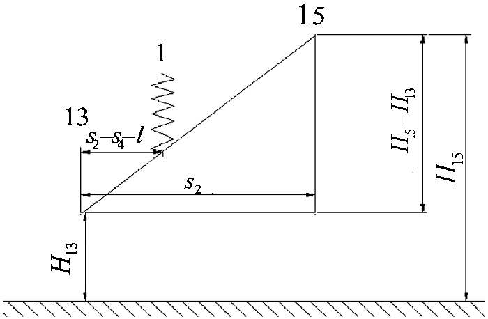
Reference height of position 1.

The height variation of secondary spring i is

$$\Delta H_1=\Delta H_{10}+\Delta z_1+\Delta h_1=w_1\cdot \Delta H_{15}+(1-w_1)\cdot \Delta H_{13}+\Delta z_1+\Delta h_1$$

(12)

$$\Delta H_2=\Delta H_{20}+\Delta z_2+\Delta h_2=w_2\cdot \Delta H_{16}+(1-w_2)\cdot \Delta H_{14}+\Delta z_2+\Delta h_2$$

(13)

$$\Delta H_{12}=\Delta H_{120}+\Delta z_{12}+\Delta h_{12}=w_{12}\cdot \Delta H_{24}+(1-w_{12})\cdot \Delta H_{22}+\Delta z_{12}+\Delta h_{12}$$

(14)

$$\{\begin{array}{l}(\Delta H_5-\Delta H_3)/(\Delta H_3-\Delta H_1)={\text{s}}_1/s_4\\ (\Delta H_6-\Delta H_4)/(\Delta H_4-\Delta H_2)={\text{s}}_1/s_4\\ (\Delta H_{11}-\Delta H_9)/(\Delta H_9-\Delta H_7)=s_4/{\text{s}}_1\\ (\Delta H_{12}-\Delta H_{10})/(\Delta H_{10}-\Delta H_8)=s_4/{\text{s}}_1\\ (\Delta H_8-\Delta H_6)/(\Delta H_6-\Delta H_4)={\text{s}}_1/2(a_1-{\text{s}}_1-s_4)\\ (\Delta H_9-\Delta H_7)/(\Delta H_7-\Delta H_5)={\text{s}}_1/2(a_1-{\text{s}}_1-s_4)\\ (\Delta H_{17}-\Delta H_{15})/(\Delta H_{15}-\Delta H_{13})={\text{s}}_3/s_2\\ (\Delta H_{18}-\Delta H_{16})/(\Delta H_{16}-\Delta H_{14})={\text{s}}_3/s_2\\ (\Delta H_{23}-\Delta H_{21})/(\Delta H_{21}-\Delta H_{19})={\text{s}}_2/s_3\\ (\Delta H_{24}-\Delta H_{22})/(\Delta H_{22}-\Delta H_{20})={\text{s}}_2/s_3\\ \Delta H_3+\Delta H_6=\Delta H_4+\Delta H_5\\ \Delta H_5+\Delta H_8=\Delta H_6+\Delta H_7\\ \Delta H_7+\Delta H_{10}=\Delta H_8+\Delta H_9\\ \Delta H_{13}+\Delta H_{18}=\Delta H_{14}+\Delta H_{17}\\ \Delta H_{19}+\Delta H_{24}=\Delta H_{20}+\Delta H_{23}\end{array}$$

(15)

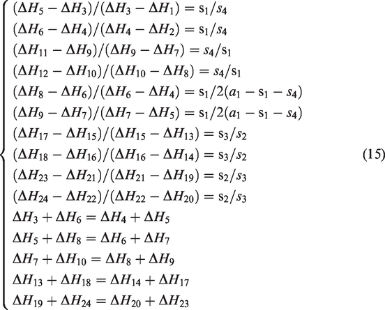
Deformation-compatibility equation (15) can be obtained via the collinear and coplanar relationship of the suspension positions.

The equation of Hooke’s law

$$F_i=k_i\cdot z_i\Rightarrow z_i=F_i/k_i=F_i\cdot c_i$$

(16)

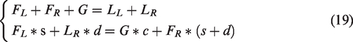
The support reaction force F_i is derived as the multivariate function of the corresponding shim quantity h_i: F_i =f(h₁, h₂,…, h_n), with the total differential of F_i expressed as follows

$$\{\begin{array}{c}\Delta F_j={\displaystyle \sum _{i=1}^n{k}_{ij}\cdot \begin{array}{c}\begin{array}{c}\Delta h_i\end{array}\end{array}},(i,j=1,2,\cdot \cdot \cdot ,n)\\ k_{ij}=\frac{\partial F_j}{\partial h_i}=\frac{\partial f_{ji}(h_i)}{\partial h_i}\end{array}$$

(17)

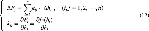
Equation (17) reveals that whether one increases the shim quantity of several suspension positions simultaneously or increases them one by one, the variation in the support reaction force is the same. Through a further calculation the load distribution of the supporting points after shimming can be obtained

$$F_j=F_{0j}+{\displaystyle \sum _{i=1}^n{k}_{ij}\cdot \Delta h_i}\hspace{1em}(i,j=1,2,\cdot \cdot \cdot ,n)$$

(18)

Equation (18) is the entire locomotive load adjustment equation, which reflects the load distribution and variation of each spring after shimming. This equation forms the theoretical basis of the proposed entire locomotive load adjustment technology. In equation (18), k_ij is the element of the influence matrix K, which reveals how the jth spring load changes when shimming on the ith supporting point. Let K=[K_11,K₁₂;K_21,K₂₂]^T(kN/mm), where K₁₁ represents the impact of secondary shimming on the secondary spring load, K₁₂ represents the influence of primary shimming on the secondary spring load, K₂₁ reflects the impact of secondary shimming on the primary spring load and K₂₂ represents the change in primary spring load when shimming on the primary positions.

Conversion model between wheel load and primary spring load

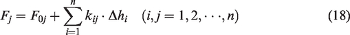
In Figure 6, G stands for the wheel load and F_L, F_R, L_L, L_R, respectively, represent the primary spring load and wheel load of the left and right sides of the same axle. All other parameters are structural parameters. The two-suspension model reveals how the primary spring load changes with shimming. To determine how the wheel load changes with shimming, the conversion model between the wheel load and primary spring load should be established. The conversion model between the wheel (axle) load and the primary spring load is derived from the statics equations (19) and the increment equation (20)

$$\{\begin{array}{l}{F}_L+F_R+G=L_L+L_R\\ F_L*\text{s}+L_R*d=G*c+F_R*(s+d)\end{array}$$

(19)

$$\Rightarrow \{\begin{array}{l}\Delta F_L+\Delta F_R=\Delta L_L+\Delta L_R\\ \Delta F_L*\text{s}+\Delta L_R*d=\Delta F_R*(s+d)\end{array}$$

(20)

$$\Rightarrow \{\begin{array}{l}\Delta L_R=\Delta F_R+(\Delta F_R-\Delta F_L)*s/d\\ \Delta L_L=\Delta F_L-(\Delta F_R-\Delta F_L)*s/d\end{array}$$

(21)

Figure 6.

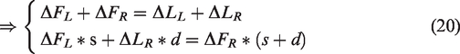
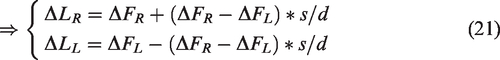
Simplified mechanical model of the wheel.

Theoretical model

In the case of a typical high-power locomotive such as the HXD1D, the value of the main structural parameters is as follows:

The influence matrix K=[K₁ K₂], which describes how the wheel load changes with shimming, can be derived based on the influence matrix K₂₁ and K₂₂ obtained in ‘Two-suspension model of a six-axle locomotive’ section and the conversion model between the wheel (axle) load and the primary spring load obtained in ‘Conversion model between wheel load and primary spring load’ section.

In the two-suspension model established in ‘Two-suspension model of a six-axle locomotive’ section, K₂₁ reflects the impact of secondary shimming on the primary spring load and K₂₂ represents the change in primary spring load when shimming on the primary positions. Substitute K₂₁, K₂₂ and the structural parameters of HXD1D locomotive in equation (21) (the conversion model between the wheel load and the primary spring load). Then, the influence matrix K=[K₁ K₂](kN/mm) of the primary and secondary shimming(mm) on the whole wheel load (kN) is established.

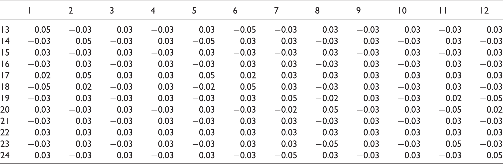
Among them, K′s element k_ij, which represents the jth column of the ith row of the matrix K, reveals how the jth wheel load changes when shimming on the ith supporting point. K₁ represents the influence of the secondary shimming on the wheel load and K₂ represents the change in the wheel load when shimming on the primary positions. K₁ and K₂ are shown in Tables 3 and 4.

Table 2.

The value of the structural parameters.

Symbol	Value	Unit
$S_{\text{1}}$	360	$\text{mm}$
$S_2$	2450	$\text{mm}$
$S_{\text{3}}$	2000	$\text{mm}$
$S_4$	360	$\text{mm}$
$a_{\text{1}}$	6413	$\text{mm}$
$l$	180	$\text{mm}$
$b$	1055	$\text{mm}$
$c_1$	0.44	$\text{mm/kN}$
$c_2$	2.236	$\text{mm/kN}$
s	305.5	$\text{mm}$
d	1499	$\text{mm}$

Table 3.

Influence matrix K1 (kN/mm) of secondary shim quantity on wheel load.

	1	2	3	4	5	6	7	8	9	10	11	12
13	0.05	−0.03	0.03	−0.03	0.03	−0.05	−0.03	0.03	−0.03	0.03	−0.03	0.03
14	−0.03	0.05	−0.03	0.03	−0.05	0.03	0.03	−0.03	0.03	−0.03	0.03	−0.03
15	0.03	−0.03	0.03	−0.03	0.03	−0.03	−0.03	0.03	−0.03	0.03	−0.03	0.03
16	−0.03	0.03	−0.03	0.03	−0.03	0.03	0.03	−0.03	0.03	−0.03	0.03	−0.03
17	0.02	−0.05	0.03	−0.03	0.05	−0.02	−0.03	0.03	−0.03	0.03	−0.03	0.03
18	−0.05	0.02	−0.03	0.03	−0.02	0.05	0.03	−0.03	0.03	−0.03	0.03	−0.03
19	−0.03	0.03	−0.03	0.03	−0.03	0.03	0.05	−0.02	0.03	−0.03	0.02	−0.05
20	0.03	−0.03	0.03	−0.03	0.03	−0.03	−0.02	0.05	−0.03	0.03	−0.05	0.02
21	−0.03	0.03	−0.03	0.03	−0.03	0.03	0.03	−0.03	0.03	−0.03	0.03	−0.03
22	0.03	−0.03	0.03	−0.03	0.03	−0.03	−0.03	0.03	−0.03	0.03	−0.03	0.03
23	−0.03	0.03	−0.03	0.03	−0.03	0.03	0.03	−0.05	0.03	−0.03	0.05	−0.03
24	0.03	−0.03	0.03	−0.03	0.03	−0.03	−0.05	0.03	−0.03	0.03	−0.03	0.05

Table 4.

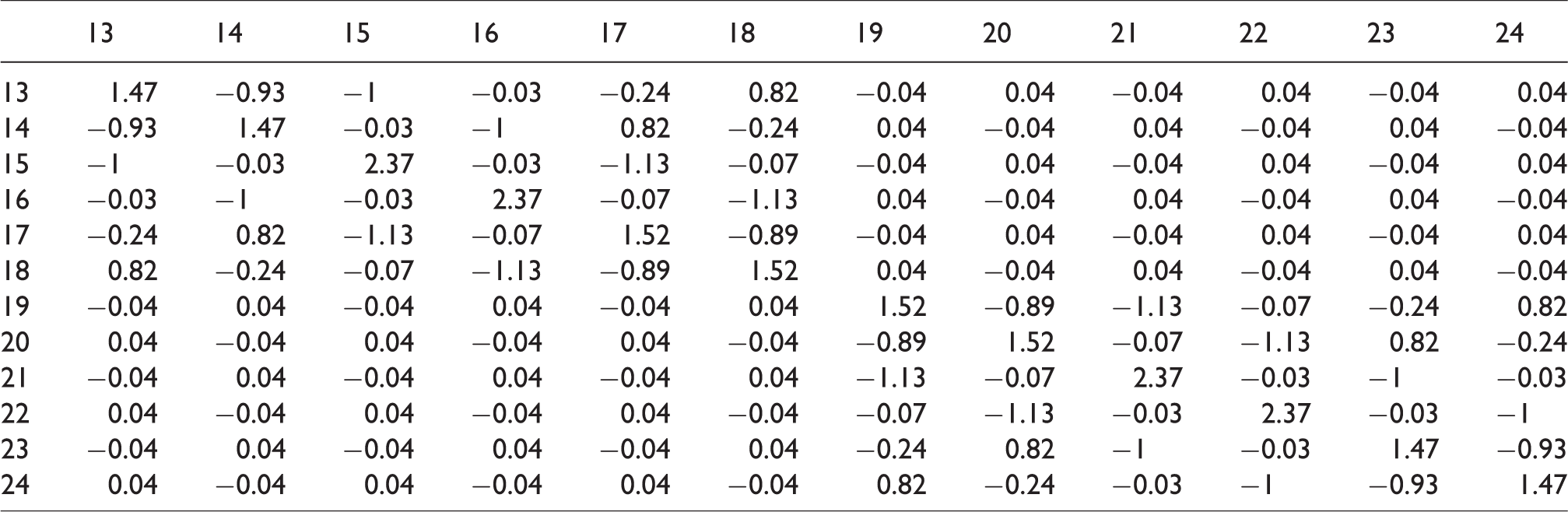
Influence matrix K2 (kN/mm) of primary shim quantity on wheel load.

	1	2	3	4	5	6	7	8	9	10	11	12
13	1.40	−1.00	−0.93	0.13	−0.33	0.73	−0.04	0.04	−0.04	0.04	−0.04	0.04
14	−1.00	1.40	0.13	−0.93	0.73	−0.33	0.04	−0.04	0.04	−0.04	0.04	−0.04
15	−0.93	0.13	2.03	−0.37	−0.96	0.11	−0.04	0.04	−0.04	0.04	−0.04	0.04
16	0.13	−0.93	−0.37	2.03	0.11	−0.96	0.04	−0.04	0.04	−0.04	0.04	−0.04
17	−0.33	0.73	−0.96	0.11	1.43	−0.98	−0.04	0.04	−0.04	0.04	−0.04	0.04
18	0.73	−0.33	0.11	−0.96	−0.98	1.43	0.04	−0.04	0.04	−0.04	0.04	−0.04
19	−0.04	0.04	−0.04	0.04	−0.04	0.04	1.43	−0.98	−0.96	0.11	−0.33	0.73
20	0.04	−0.04	0.04	−0.04	0.04	−0.04	−0.98	1.43	0.11	−0.96	0.73	−0.33
21	−0.04	0.04	−0.04	0.04	−0.04	0.04	−0.96	0.11	2.03	−0.37	−0.93	0.13
22	0.04	−0.04	0.04	−0.04	0.04	−0.04	0.11	−0.96	−0.37	2.03	0.13	−0.93
23	−0.04	0.04	−0.04	0.04	−0.04	0.04	−0.33	0.73	−0.93	0.13	1.40	−1.00
24	0.04	−0.04	0.04	−0.04	0.04	−0.03	0.73	−0.33	0.13	−0.93	−1.00	1.40

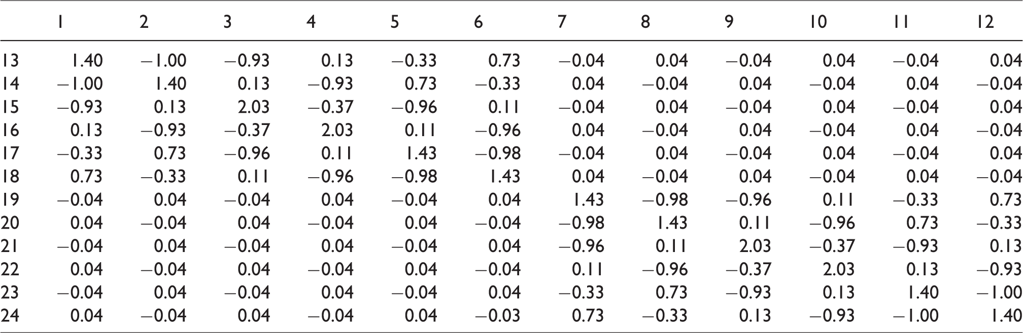
In this case, K₁ (kN/mm) represents the impact of secondary shim quantity on wheel load, while K₂ (kN/mm) represents the influence of primary shimming on wheel load.

Considering the highly symmetric structure of the system in question, the application of shimming on the symmetric positions has the same impact on wheel load in high-power locomotives. For the described influence matrices, the impact of primary shimming on wheel load is obviously greater than that of secondary shimming. Furthermore, as the primary shimming process on site can be realised more easily, primary shimming should be considered a priority.

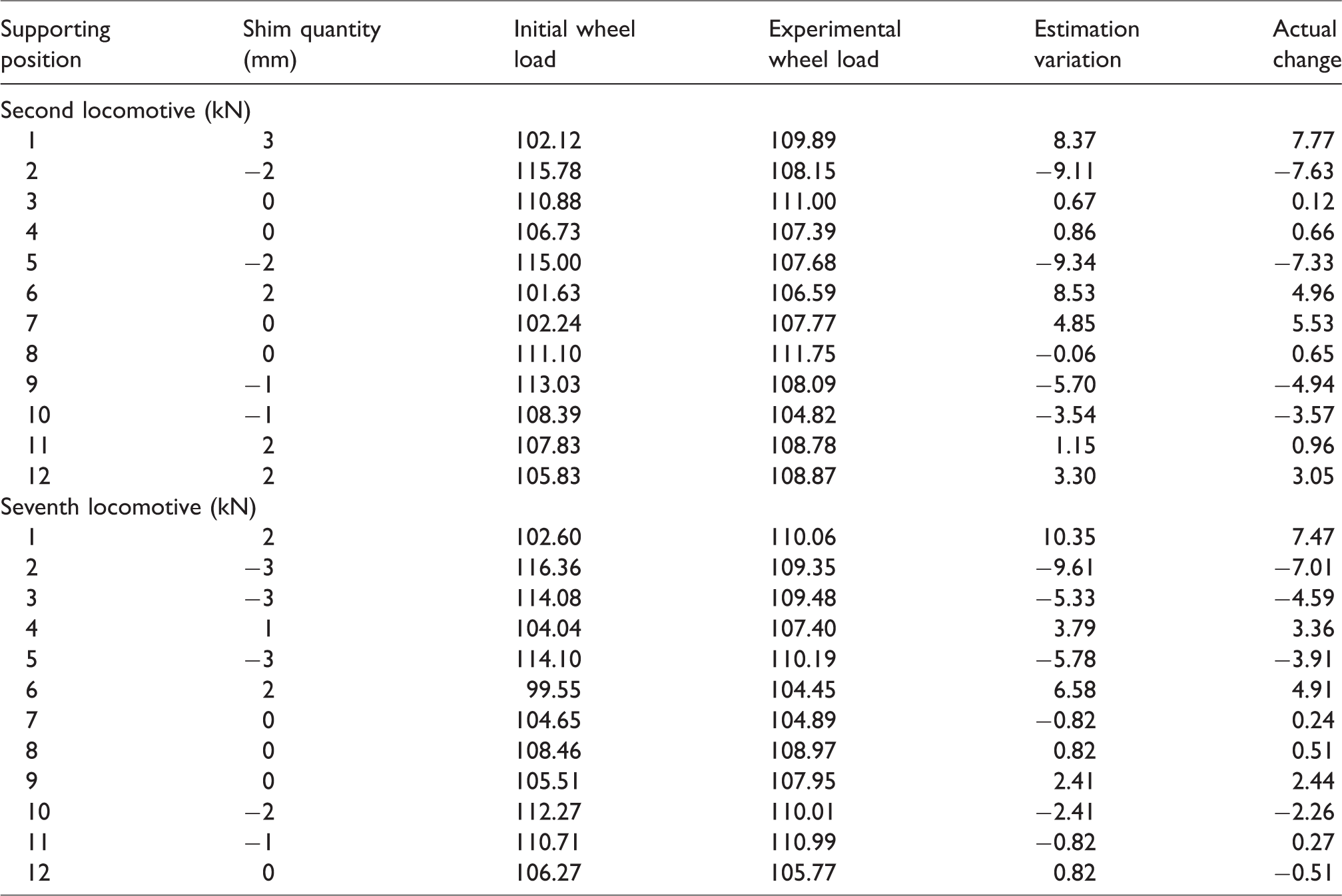
To verify the theoretical model, results obtained via theoretical calculation were compared with those obtained via a series of experiments. A total of 10 locomotives took part in the initial load adjustment tests, with the second and seventh randomly selected for analysis.

Analysis of Table 5 reveals that the trend of estimation variation is the same as that of the actual change. Thus, the proposed theoretical estimation method is able to accurately reflect the variation in wheel load after shimming. The table also presents the influence of the shim quantity on the wheel load; this parameter is thus an important reference for load adjustment tests and can greatly reduce modelling error.

Table 5.

Comparison between theoretical calculation and experimental results.

Supporting position	Shim quantity (mm)	Initial wheel load	Experimental wheel load	Estimation variation	Actual change
Second locomotive (kN)
1	3	102.12	109.89	8.37	7.77
2	−2	115.78	108.15	−9.11	−7.63
3	0	110.88	111.00	0.67	0.12
4	0	106.73	107.39	0.86	0.66
5	−2	115.00	107.68	−9.34	−7.33
6	2	101.63	106.59	8.53	4.96
7	0	102.24	107.77	4.85	5.53
8	0	111.10	111.75	−0.06	0.65
9	−1	113.03	108.09	−5.70	−4.94
10	−1	108.39	104.82	−3.54	−3.57
11	2	107.83	108.78	1.15	0.96
12	2	105.83	108.87	3.30	3.05
Seventh locomotive (kN)
1	2	102.60	110.06	10.35	7.47
2	−3	116.36	109.35	−9.61	−7.01
3	−3	114.08	109.48	−5.33	−4.59
4	1	104.04	107.40	3.79	3.36
5	−3	114.10	110.19	−5.78	−3.91
6	2	99.55	104.45	6.58	4.91
7	0	104.65	104.89	−0.82	0.24
8	0	108.46	108.97	0.82	0.51
9	0	105.51	107.95	2.41	2.44
10	−2	112.27	110.01	−2.41	−2.26
11	−1	110.71	110.99	−0.82	0.27
12	0	106.27	105.77	0.82	−0.51

Tread measured model

Although the theoretical model considers the locomotive body and bogie as rigid bodies, they are actually susceptible to small deformations when bearing extreme loads. As a result, the theoretical estimation variation exhibited deviation from the experimental results and it is necessary to further perfect the model by establishing a tread measured model.

The influence matrix of tread shimming on wheel load 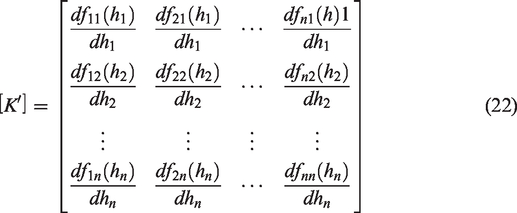$K^{\prime }$ was obtained based on experiments involving the application of shimming on the tread

$$\left[K^{\prime }\right]=\left[\begin{array}{cccc}\frac{d{f}_{11}(h_1)}{d{h}_1}& \frac{d{f}_{21}(h_1)}{d{h}_1}& \cdots & \frac{d{f}_{n1}(h)1}{d{h}_1}\\ \frac{d{f}_{12}(h_2)}{d{h}_2}& \frac{d{f}_{22}(h_2)}{d{h}_2}& \cdots & \frac{d{f}_{n2}(h_2)}{d{h}_2}\\ ⋮& ⋮& ⋮& ⋮\\ \frac{d{f}_{1n}(h_n)}{d{h}_n}& \frac{d{f}_{2n}(h_n)}{d{h}_n}& \cdots & \frac{d{f}_{nn}(h_n)}{d{h}_n}\end{array}\right]$$

(22)

For a known initial wheel load, matrix $K^{\prime }$ can be used as the measured model to calculate the shim quantity the treads require for uniformity of wheel load. Then, the primary shimmed quantity, which is used to guide field production, can be obtained via the conversion model between the shim quantity on treads and that on the primary supporting positions. Considering the fact that the building process of the tread measured model suffers from being rather time consuming, it is unnecessary to establish the tread measured model if the deviation exhibited by the theoretical calculation result is acceptable.

Table 6 shows the comparison between the modified estimation variation and the unmodified variation, with the second and seventh locomotives (randomly selected from 10 locomotives) for analysis.

Table 6.

Comparison between the modified estimation variation and the unmodified variation.

Supporting position	Shim quantity (mm)	Unmodified estimation variation	Modified estimation variation	Actual change
Second locomotive (kN)
1	3	8.37	7.98	7.77
2	−2	−9.11	−8.16	−7.63
3	0	0.67	0.21	0.12
4	0	0.86	0.61	0.66
5	−2	−9.34	−8.69	−7.33
6	2	8.53	6.12	4.96
7	0	4.85	5.69	5.53
8	0	−0.06	0.47	0.65
9	−1	−5.70	−4.79	−4.94
10	−1	−3.54	−3.56	−3.57
11	2	1.15	0.87	0.96
12	2	3.30	2.96	3.05
Seventh locomotive (kN)
1	2	10.35	8.49	7.47
2	−3	−9.61	−6.74	−7.01
3	−3	−5.33	−5.07	−4.59
4	1	3.79	3.62	3.36
5	−3	−5.78	−4.51	−3.91
6	2	6.58	5.47	4.91
7	0	−0.82	−0.28	0.24
8	0	0.82	0.71	0.51
9	0	2.41	2.51	2.44
10	−2	−2.41	−2.19	−2.26
11	−1	−0.82	−0.19	0.27
12	0	0.82	0.21	−0.51

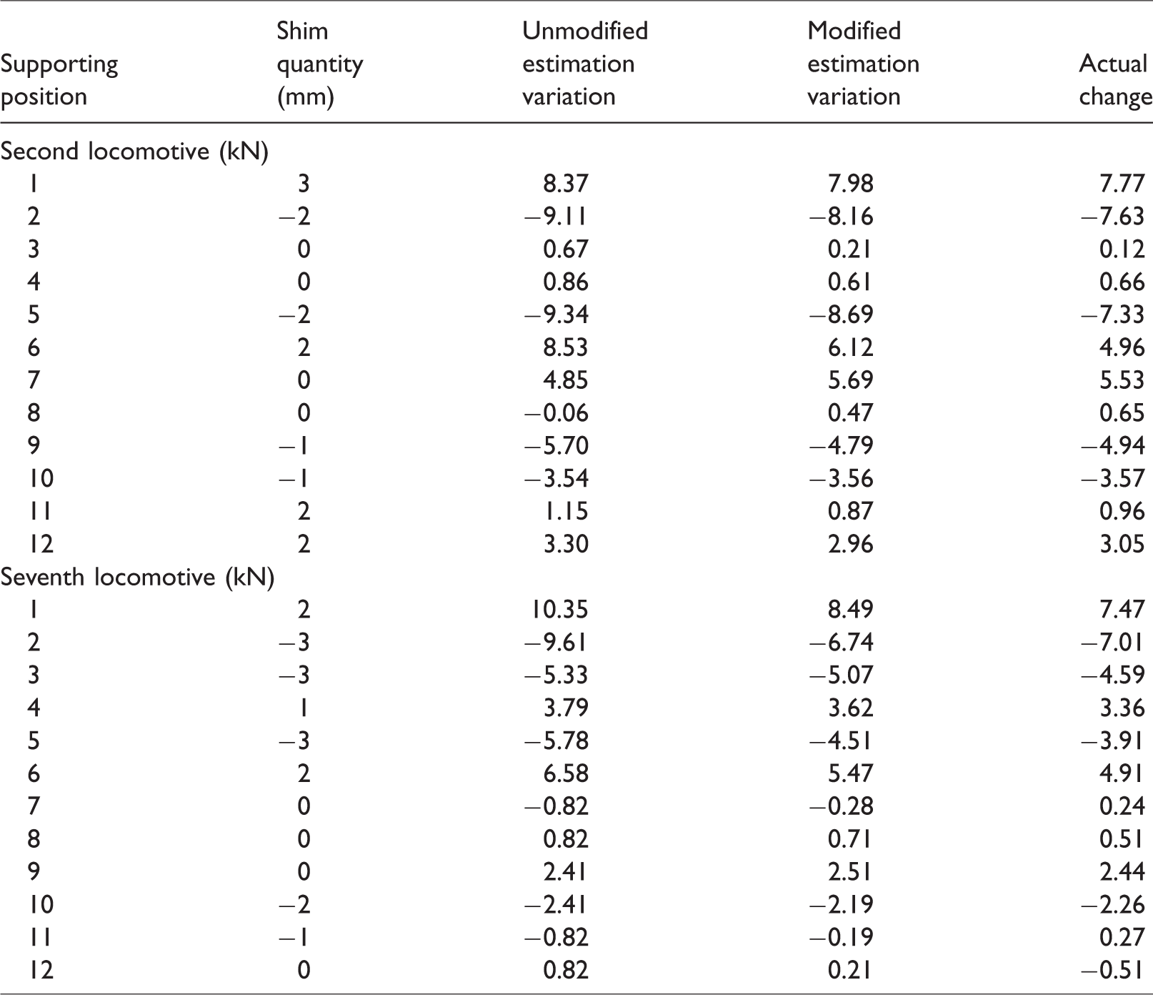
As shown in Table 6, the modified estimation variation obtained by the tread measured model is closer to the actual change than the unmodified estimation variation.

Conversion model between primary and tread shim quantities

If the deviation exhibited by theoretical calculation results cannot be neglected, then the tread measured model must be established. By controlling the vertical displacement of the test bed of entire locomotive load adjustment, the tread height variation and resulting wheel load change can be measured. Meanwhile, the tread measured composite stiffness can be obtained using equation (22). On the basis of equation (18), the tread shim quantity required to control the wheel (axle) load distribution within the scope of corresponding standards can be obtained, with the tread lifting steps controlled via a nonlinear electro-hydraulic actuator. In order to guide field production, the tread shim quantity should be converted to the primary spring shim quantity, as the conversion model shown in Figure 7.

Figure 7.

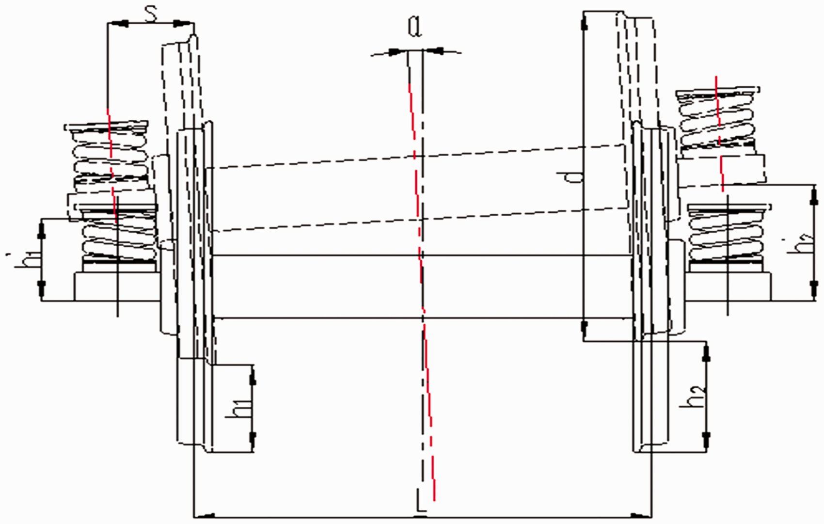
Conversion model between the tread and primary shim quantities.

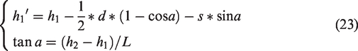
The primary spring is also susceptible to the rotary motion of the locomotive wheel (axle) after shimming on the tread. As shown in Figure 7, h₁ and h₂, respectively, represent the tread shim quantities for the two ends of the axle; h₁′ and h₂′ represent the primary shim quantities for the two ends of the axle; α represents the dip caused by shimming on the tread and S represents the axial distance from the roller surface to the spring seat. The conversion formula for the tread and primary shim quantities is

$$\{\begin{array}{l}{h}_1\prime =h_1-\frac{1}{2}*d*(1-\cos a)-s*\sin a\\ \tan \hspace{0.17em}a=(h_2-h_1)/L\end{array}$$

(23)

where dip α is very small and therefore $\cos \hspace{0.17em}a\hspace{0.17em}\approx \hspace{0.17em}1$ and $\sin \hspace{0.17em}a\hspace{0.17em}\approx \hspace{0.17em}\tan a$ . As a result, the conversion formula of the first position can be simplified via equation as follows

$$h_1\prime =h_1-s*(h_2-h_1)/L$$

(24)

Equation (25) expresses the relationship between the primary spring shim quantities for two ends of the axle

$$h_2\prime -h_1\prime =(2s+\text{L})*\sin \hspace{0.17em}a=(2s+\text{L})*(h_2-h_1)/L$$

(25)

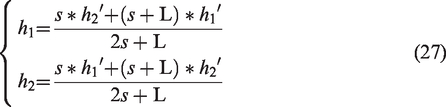
Then, the conversion formula for the second position is expressed as in equation (26)

$$h_2\prime \text{=}{h}_1\prime +(2s+\text{L})*\sin \hspace{0.17em}a=h_2+s*(h_2-h_1)/L$$

(26)

The conversion model between the tread and primary shim quantities is obtained as shown in equation (27)

$$\{\begin{array}{l}{h}_1\text{=}\frac{s*h_2\prime \text{+(}s+\text{L})*h_1\prime }{2s+\text{L}}\\ h_2\text{=}\frac{s*h_1\prime \text{+(}s+\text{L})*h_2\prime }{2s+\text{L}}\end{array}$$

(27)

Based on equation (18), the influence matrix of tread shim quantity on wheel load distribution K′ (kN/mm) is obtained by combining equations (21), (24) and (25). Matrix K′ illustrates how the wheel load changes with the shimming process carried out on the tread.

Tables 4 and 7 reveal that although the trends of the respective influences of the primary and tread shimming processes on wheel load are the same, the tread shimming process has a greater overall impact.

With matrix K′, the tread shim quantity required to control the wheel (axle) load distribution within the scope of corresponding standards can be obtained easily.

Table 7.

Influence matrix ( $K^{\prime }$ ) (kN/mm) of tread shim quantity on wheel load.

	13	14	15	16	17	18	19	20	21	22	23	24
13	1.47	−0.93	−1	−0.03	−0.24	0.82	−0.04	0.04	−0.04	0.04	−0.04	0.04
14	−0.93	1.47	−0.03	−1	0.82	−0.24	0.04	−0.04	0.04	−0.04	0.04	−0.04
15	−1	−0.03	2.37	−0.03	−1.13	−0.07	−0.04	0.04	−0.04	0.04	−0.04	0.04
16	−0.03	−1	−0.03	2.37	−0.07	−1.13	0.04	−0.04	0.04	−0.04	0.04	−0.04
17	−0.24	0.82	−1.13	−0.07	1.52	−0.89	−0.04	0.04	−0.04	0.04	−0.04	0.04
18	0.82	−0.24	−0.07	−1.13	−0.89	1.52	0.04	−0.04	0.04	−0.04	0.04	−0.04
19	−0.04	0.04	−0.04	0.04	−0.04	0.04	1.52	−0.89	−1.13	−0.07	−0.24	0.82
20	0.04	−0.04	0.04	−0.04	0.04	−0.04	−0.89	1.52	−0.07	−1.13	0.82	−0.24
21	−0.04	0.04	−0.04	0.04	−0.04	0.04	−1.13	−0.07	2.37	−0.03	−1	−0.03
22	0.04	−0.04	0.04	−0.04	0.04	−0.04	−0.07	−1.13	−0.03	2.37	−0.03	−1
23	−0.04	0.04	−0.04	0.04	−0.04	0.04	−0.24	0.82	−1	−0.03	1.47	−0.93
24	0.04	−0.04	0.04	−0.04	0.04	−0.04	0.82	−0.24	−0.03	−1	−0.93	1.47

Optimisation algorithm for entire locomotive load adjustment based on QPSO and AGA (QAGA)

Locomotive load regulation is a nonlinear multi-objective problem, ¹⁶ with entire locomotive load adjustment involving the optimisation of the shim quantity, the number of shimming positions, maximum load difference and load variance. In this regard, the present paper proposes QAGA, an optimisation method combining QPSO algorithm and AGA. The QPSO position update equation improves the efficiency and population distribution, while the AGA genetic operation, designed to perform crossover and mutation operations on individuals with higher fitness, is employed to enrich sample diversity and improve accuracy.

Mathematical model of optimisation for entire locomotive load adjustment

$$\{\begin{array}{l}\text{min}\left\{J_{\text{1}}\text{=}{\sigma }_F\text{,}{J}_{\text{2}}\text{=Pos,}{J}_{\text{3}}\text{=Sum}\right\}\\ F_j\text{=}{F}_{\text{0}j}+{\displaystyle \sum _{i=1}^n{k}_{ij}\times h_i,{\sigma }_F=\frac{1}{n-1}{\displaystyle \sum _{j=1}^n{(F_j-\stackrel{-}{F})}^2}}\\ \text{Pos=}{\displaystyle \sum _{i\text{=1}}^n\left[\{\begin{array}{l}\begin{array}{cc}\text{0}& h_i\text{=0}\end{array}\\ \begin{array}{cc}\text{1}& h_i\ne \text{0}\end{array}\end{array}\right]},\text{Sum=}{\displaystyle \sum _{i\text{=1}}^n{h}_i}\text{,0}\le h_i\le H_{\text{max}}\text{(i,j=1,2,}\cdot \cdot \cdot \text{,}n\text{)}\end{array}$$

(28)

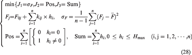
Load distribution adjustment can be realised by minimising the variance of wheel (axle) load σ_F, while the shim quantity can be controlled by minimising the total number of shimmed positions Pos and the total shim quantity Sum. Sum and Pos are indexes for shim quantity control. Three types of optimisation index are typically considered: J₁(ΔF_max), J₂(Pos) and J₃(Sum). In this case the mathematical model for entire locomotive load adjustment can be expressed in equation (28), where F_j represents the secondary spring load on the jth supporting point; $\overline{F}$ is the average secondary spring load; F_{0 j} is the secondary spring load on the jth supporting point before shimming; k_ij is the slope of the influence line depicting the change in the jth secondary spring load after shimming on the ith point; and H_max represents the maximum shim quantity allowed on a supporting point, here taken as H_max =10.

Objective function value calculation

The preference sequence of the objective functions is $J_1$ ( $J_2$ ∼ $J_3$ ), operator and stand for the degree of preference. It can be seen that the load distribution index $J_1$ is more significant than the shim quantity indexes $J_2$ and $J_3$ while $J_2$ and $J_3$ have the same status. Experiments show that the control of the total shim quantity $J_3$ can be equivalent to the control of $J_2$ , the total number of the shimmed supporting points.

According to the analysis above, the adjustment algorithm can be designed into a two-level optimisation structure:

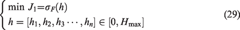
The first level: the load variance adjustment. An optimal solution set of the needed shim quantity sequence is obtained in this level. The solution set with permitted load variance is defined as, which restricts the range of feasible solution in the next level.

The optimisation goal of this level is shown in equation (29)

$$\{\begin{array}{l}\text{min}{J}_{\text{1}}\text{=}{\sigma }_F(h)\\ h=\left[h_1,h_2,h_3\cdots ,h_n\right]\in [0,H_{\max }]\end{array}$$

(29)

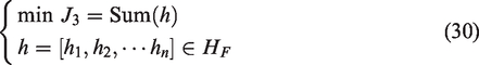
The second level: the shim quantity optimisation. The solution set H_F would be regarded as the feasible region if $\forall h\in H_F:\left|\right|{\sigma }_F(h)-{\sigma }_F^{*}\left|\right|\le {\delta }_{H_F}$ , where ‖·‖ is the Euclidean geometry distance, ${\sigma }_F^{*}$ is the feasible region centre ${\delta }_{H_F}$ and is the radius of the feasible region. This feasible region is the producing range of feasible solutions here, and the shim quantity is controlled within the range.

The optimisation goal of this level is shown in equation (30)

$$\{\begin{array}{l}\min J_3=\text{Sum}(h)\hfill \\ h=[h_1,h_2,\cdots h_n]\in H_F\hfill \end{array}$$

(30)

Wave function-based QPSO

In the QPSO system, the particle state is determined by the wave function ψ(X,t). The square of the wave function, |ψ| ² , here denoted as Q, is the probability density function of the particle position, and represents the probability density of particles appearing at spatial point X at time t.^17–19 As shown in equation (31)

$$\{\begin{array}{l}\psi (x_{ij}(t+1))=\frac{1}{\sqrt{L_{ij}(t)}}\exp \left(\frac{-\left|x_{ij}(t+1)-p_{ij}(t)\right|}{L_{ij}(t)}\right)\\ p_{ij}=\frac{c_1{r}_{1}pbes{t}_{ij}(t)+c_2{r}_{2}gbes{t}_{ij}(t)}{c_1{r}_1+c_2{r}_2}\\ L_{ij}(t)=2\alpha \cdot \left|M_j(t)-x_{ij}(t)\right|\\ Q(x_{ij}(t+1))={\left|\psi (x_{ij}(t+1))\right|}^2\\ {\displaystyle {\int }_{-\infty }^{+\infty }{\left|\psi \right|}^2}\mathrm{d}x\mathrm{d}y\mathrm{d}z={\displaystyle {\int }_{-\infty }^{+\infty }Q}\mathrm{d}x\mathrm{d}y\mathrm{d}z=1\\ x_{ij}(t+1)=p_{ij}(t)\pm \frac{L_{ij}(t)}{2}\ln (1/u_{ij}(t))\\ r_1,r_2,c_1,c_2,u_{ij}(t)\in U(0,1)\end{array}$$

(31)

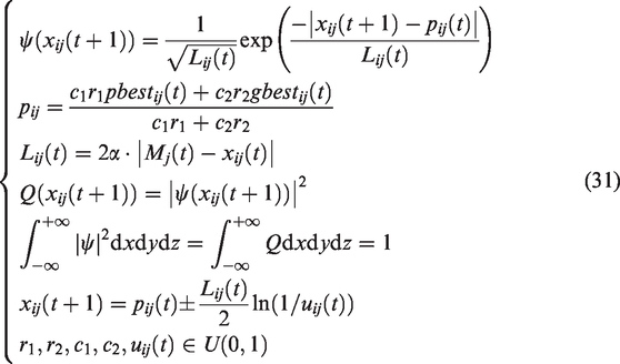
M_j(t) is the average of all particles’ optimal positions, $S$ is the population size, p_ij is component j of particle i, and c₁ and c₂ are acceleration coefficients or learning factors that are used to adjust the maximum step size between the particle and the individual or global optimal position. The particle position renewal equation is expressed as follows

$$x_{ij}(t+1)=p_{ij}(t)\pm \alpha \cdot \left|M_j(t)-x_{ij}(t)\right|\cdot \ln (1/u_{ij}(t))$$

(32)

where α is a compression expansion factor that adjusts the speed of particle convergence. This is the only parameter in the QPSO algorithm, with the exception of the number of iterations and the size of the population. Earlier research undertaken by Sun et al. ²⁰ has shown that the algorithm converges when α＜1.78. The current optimal position of particle P_ji and the optimal population location P_g are updated as follows

$$\{\begin{array}{l}{P}_{ij}(t+1)=\{\begin{array}{l}{P}_{ij}(t)\begin{array}{ccc}& if& f(x_{ij}(t+1))\ge \end{array}f(P_{ij}(t))\\ x_{ij}(t+1)\begin{array}{ccc}& if& f(x_{ij}(t+1))<f(P_{ij}(t))\end{array}\end{array}\\ P_g(t+1)=\arg \min \begin{array}{c}f(P_g(t+1))\end{array}\end{array}$$

(33)

AGA based on degree of convergence

Genetic coding

Considering that the total number of locomotive supporting positions is very large (generally), which will produce a huge variable dimension, it is better to employ decimal number genetic coding for the chromosome rather than binary genetic coding. ²¹ Here the chromosome is defined as a_i=[h₁,h₂,…,h_n] (where n is the total number of lifting positions and h_i is defined on the interval [0,10]), with h_i representing the code for the shim quantity on the ith lifting position.

Definition 1: The average fitness of individuals is set as f_t. f_max represents the optimal individual fitness and f represents the average fitness value of all particles with fitness greater than f_t. Then, the degree of population convergence is defined as Δ= f_max − f. Then the formula for calculating the AGA crossover and mutation probability is

$$\{\begin{array}{l}{P}_c=-1/(1+\exp (-k_1·\Delta ))+1.5\\ P_m=-1/(1+\exp (-k_2·\Delta ))+1\end{array}$$

(34)

where k₁ and k₂ are positive constants, and Δ is non-negative. As a result, the range of the crossover probability P_g is [0.5,1], while the range of the mutation probability P_m is [0,0.5]. In the traditional algorithm, control parameters such as the crossover and mutation probabilities are independent of the population evolution process, and thus this fixed parameter control mechanism can lead to premature convergence.^22,23 In the proposed algorithm, however, the crossover probability P_g and mutation probability P_m are adjusted automatically according to the degree of population convergence Δ.

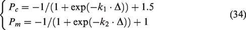
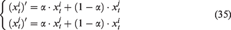
Genetic operator

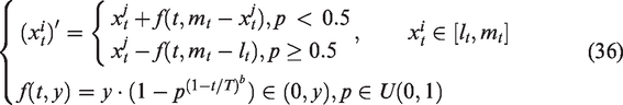
The crossover and mutation of the AGA proposed in this paper are based on arithmetic crossover and non-uniform mutation, as expressed in equations (35) and (36), respectively

$$\{\begin{array}{l}(x_t^i{)}^{\prime }=\alpha \cdot x_t^i+(1-\alpha )\cdot x_t^j\\ (x_t^j{)}^{\prime }=\alpha \cdot x_t^j+(1-\alpha )\cdot x_t^i\end{array}$$

(35)

$$\{\begin{array}{l}(x_t^i{)}^{\prime }=\{\begin{array}{l}{x}_t^j+f(t,m_t-x_t^j),p<0.5\\ x_t^j-f(t,m_t-l_t),p\ge 0.5\end{array},x_t^i\in \left[l_t,m_t\right]\\ f(t,y)=y\cdot (1-p^{{(1-t/T)}^b})\in \left(0,y\right),p\in U\left(0,1\right)\end{array}$$

(36)

where α is a random number with the value range (0,1), T is the maximum number of iterations, parameter b determines the non-uniformity of the mutation operation and F is an adaptive mutation operator that can adaptively adjust the step size. F is used to search potential regions in the whole domain, but in the later stages of iteration only a small neighbouring area of the current solution is searched so as to ensure the accurate positioning and locking of the optimal solution.

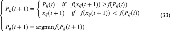
Fitness function and fitness evaluation

Fitness selection is based on the ranking evaluation method and a population size of N. Here the objective function values are calculated according to equation (28), with the smaller value of the target function, the larger the individual’s order. Let N be the population size and let Rank be the individual’s serial number in the population. Setting S_p∈[1.0,2.0] as the selection pressure, the fitness function can then be expressed as

$$\text{Fit}\left(x_i\right)=2-{\text{S}}_{\text{p}}+\frac{2\left({\text{S}}_{\text{p}}-1\right)\left(\text{Rank}-\text{1}\right)}{\text{N}-1}$$

(37)

The evaluation process proceeds as follows

Calculate the objective function values J₁(xj) and J₃(x_j)( j = 1,2,…,M) according to equations (29) and (30).

Arrange the population in descending order based on the first preferential objective function J₁. If two or more individuals share the same value of J₁, arrange them in descending order based on the second preferential objective function J₃. If any individuals share the same value of both J₁ and J₃, rank these individuals randomly.

The fitness value is then assigned to each individual based on equation (37), with Rank=M representing the optimal individual and Rank = 1 representing the worst individual.

Flow of the QAGA algorithm

Sample initialisation: Set S as the sample number and T as the maximum number of iterations. Randomly generate S samples $x_0^i$ $(i=1,2,\cdots ,\text{S)}$ .

Objective function value calculation: Calculate the objective function values. Obtain the total number of shimmed positions Pos, the total shim quantity Sum and the variance of the wheel (axle) load σF.

Sample update via QPSO: Update the sample according to the QPSO position update equation.

Fitness evaluation: Rank the population according to the objective function values. A fitness value is then assigned to each individual based on equation (37).

Adaptive genetic operation: Eliminate individuals with lower fitness and replace them with the same number of individuals with higher fitness. Then, introduce the AGA arithmetic crossover and non-uniform mutation to enrich sample diversity and improve accuracy.

Output results: Stop the iteration and output the shimming positions, the shim quantity and the load variance when it comes to the iterative termination conditions. Otherwise, return to Step 2.

The flow chart for the QAGA algorithm is shown in Figure 8.

Figure 8.

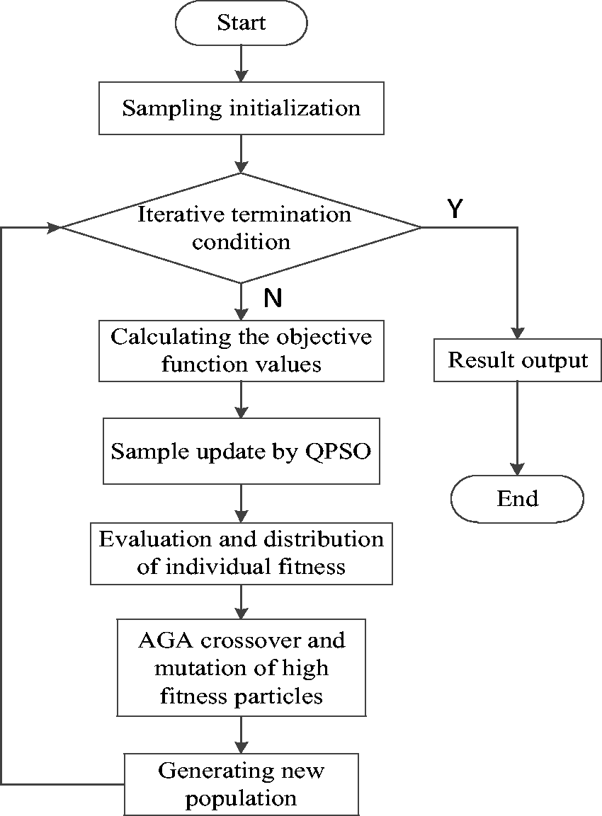
Flow chart for the QAGA algorithm.

Example and application results

Load distribution optimisation results

QAGA optimisation algorithm was used in a simulation of entire locomotive load adjustment using data for an HXD1D-type locomotive, which has 12 primary lifting points and 12 secondary lifting points.

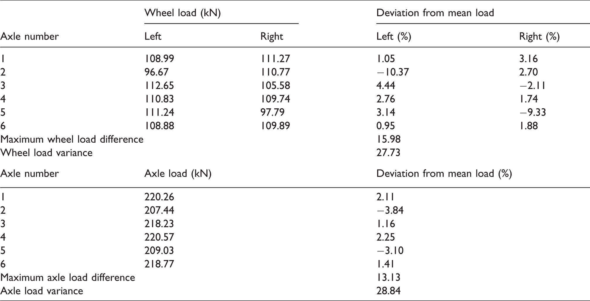
The influence matrix K₂ can be obtained as shown in Table 4. Analysis of this matrix reveals that the influence on wheel load of shimming on a single supporting position is greater than 1.40 kN/mm, which means that, within the permissible limit of shim quantity (10 mm), the maximum impact of shimming on locomotive wheel load is 14 kN, or 13% of the average wheel load. Similarly, the influence on axle load of shimming on a single supporting position is more than 0.39 kN/mm, which means that the maximum impact of the shimming process on locomotive axle load is 3.9 kN, or 1.8% of the average axle load. The wheel (axle) load difference did not exceed the scope of the corresponding standards; the analysed tread shimming process is quite efficient in wheel load and axle load adjustment. In order to verify the proposed method’s practical application, a simulation was carried out examining the most difficult adjustment situation possible, i.e. that the wheel load and axle load distribution both exceed the scope of corresponding standards. The initial load distribution under entire locomotive conditions is shown in Table 8.

Table 8.

Initial entire locomotive load distribution of the HXD1D locomotive.

	Wheel load (kN)		Deviation from mean load
Axle number	Left	Right	Left (%)	Right (%)
1	108.99	111.27	1.05	3.16
2	96.67	110.77	−10.37	2.70
3	112.65	105.58	4.44	−2.11
4	110.83	109.74	2.76	1.74
5	111.24	97.79	3.14	−9.33
6	108.88	109.89	0.95	1.88
Maximum wheel load difference			15.98
Wheel load variance			27.73
Axle number	Axle load (kN)		Deviation from mean load (%)
1	220.26		2.11
2	207.44		−3.84
3	218.23		1.16
4	220.57		2.25
5	209.03		−3.10
6	218.77		1.41
Maximum axle load difference			13.13
Axle load variance			28.84

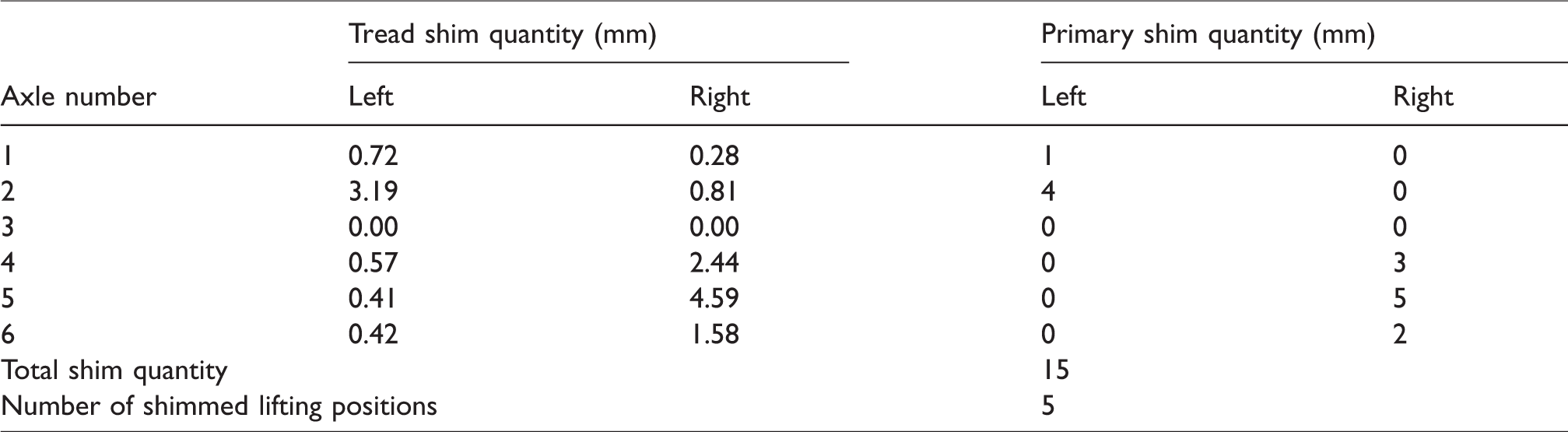
As shown in Table 9, the tread shim quantity and the corresponding primary shim quantity were obtained using the proposed QAGA optimisation theory. The shimming process was repeated according to the obtained optimisation results, with the new distribution of the entire locomotive wheel (axle) load obtained as shown in Table 10.

Table 9.

QAGA-derived optimisation results for HXD1D shim quantity.

	Tread shim quantity (mm)		Primary shim quantity (mm)
Axle number	Left	Right	Left	Right
1	0.72	0.28	1	0
2	3.19	0.81	4	0
3	0.00	0.00	0	0
4	0.57	2.44	0	3
5	0.41	4.59	0	5
6	0.42	1.58	0	2
Total shim quantity			15
Number of shimmed lifting positions			5

Table 10.

Adjusted results of entire locomotive load distribution for the HXD1D locomotive.

	Wheel load (kN)		Deviation from mean load
Axle number	Left	Right	Left (%)		Right (%)
1	108.02	109.34	0.15		1.37
2	105.08	108.50	−2.58		0.59
3	108.18	106.69	0.30		−1.08
4	109.67	107.33	1.68		−0.49
5	108.83	107.12	0.90		−0.68
6	109.46	106.05	1.49		−1.68
Maximum wheel load difference				4.59
Wheel load variance				2.06
Axle number	Axle load (kN)		Deviation from mean load (%)
1	217.36		0.76
2	213.58		−0.99
3	214.87		−0.39
4	217.00		0.60
5	215.95		0.11
6	215.51		−0.09
Maximum load difference				3.78
load variance				1.62

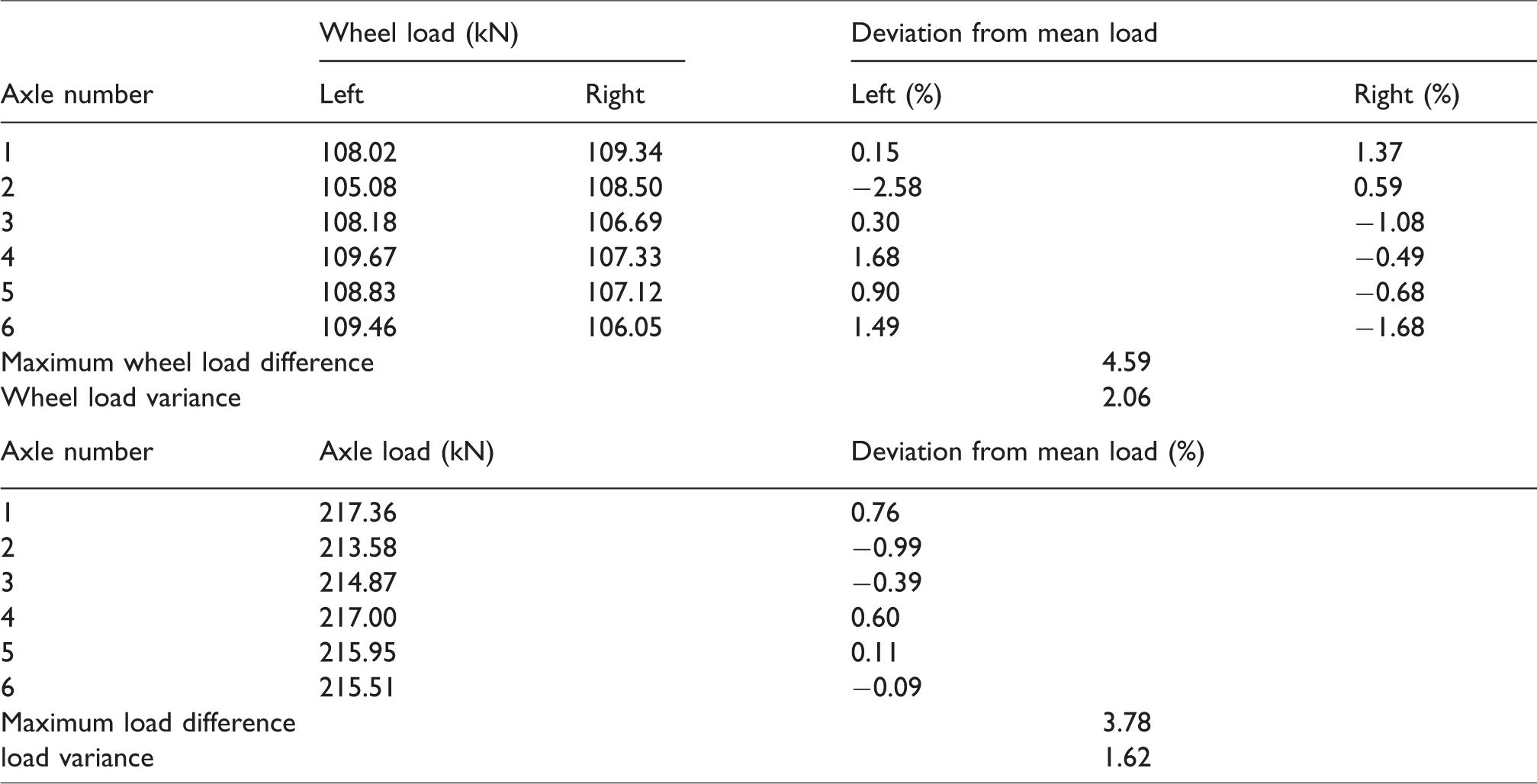
A comparison of Tables 8 and 10 reveals that the tread shimming process under entire locomotive conditions has a considerable impact on the entire locomotive wheel (axle) load distribution, with the maximum deviation of wheel (axle) load $\Delta F_{\max }$ successfully reduced to within the permissible limit of ±4% (±2%). In conclusion, shimming on treads under entire locomotive conditions is an efficient method for the adjustment of wheel (axle) load distribution.

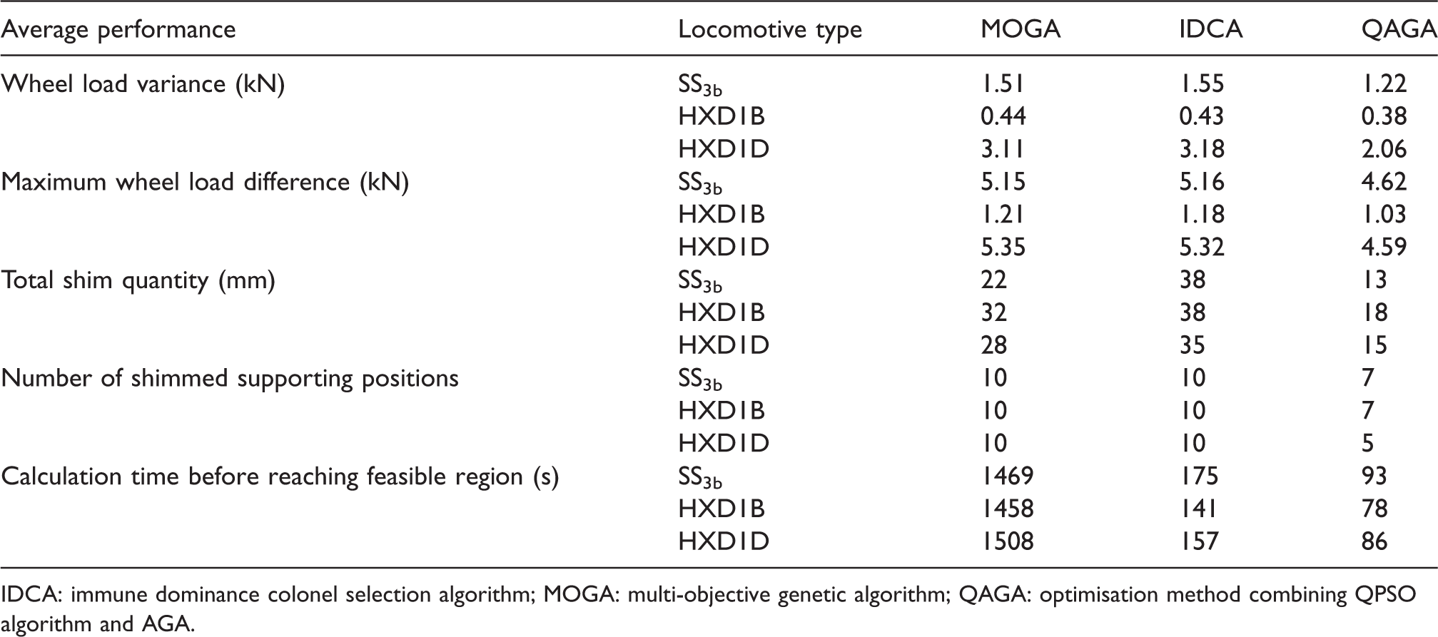
As can be seen from Table 11, the load variance achieved by the QAGA algorithm was the smallest. In terms of shim quantity control, the QAGA algorithm also performed much better than both the multi-objective genetic algorithm (MOGA) and immune dominance colonel selection algorithm (IDCA) methods, reducing the total shim quantity with respect to that achieved using these two algorithms by 41 and 66% (SS3b), 44 and 53% (HXD1B), and 46 and 57% (HXD1D), respectively. Furthermore, the number of un-shimmed supporting points was reduced by 30% (SS3b and HXD1B) and 50% (HXD1D), respectively. In addition, compared with that of the MOGA and IDCA methods, the solving efficiency of QAGA is considerably better, with calculation time reduced by 94 and 47% (SS3b), 95 and 45% (HXD1B) and 94 and 45% (HXD1D), respectively. In summary, QAGA offers effective shim quantity control together with effective locomotive load adjustment ability and high solving efficiency. Compared with other similar algorithms, the QAGA method greatly reduces the shim quantity and calculation time; in brief, its overall performance is simply better.

Table 11.

Performance comparison of MOGA, IDCA and QAGA.

Average performance	Locomotive type	MOGA	IDCA	QAGA
Wheel load variance (kN)	SS3b	1.51	1.55	1.22
	HXD1B	0.44	0.43	0.38
	HXD1D	3.11	3.18	2.06
Maximum wheel load difference (kN)	SS3b	5.15	5.16	4.62
	HXD1B	1.21	1.18	1.03
	HXD1D	5.35	5.32	4.59
Total shim quantity (mm)	SS3b	22	38	13
	HXD1B	32	38	18
	HXD1D	28	35	15
Number of shimmed supporting positions	SS3b	10	10	7
	HXD1B	10	10	7
	HXD1D	10	10	5
Calculation time before reaching feasible region (s)	SS3b	1469	175	93
	HXD1B	1458	141	78
	HXD1D	1508	157	86

IDCA: immune dominance colonel selection algorithm; MOGA: multi-objective genetic algorithm; QAGA: optimisation method combining QPSO algorithm and AGA.

Variation in shim quantity and number of shimmed positions

Figure 9 shows the change in the second preferential objective value (total shim quantity and the number of shimmed supporting positions) for an HXD1D-type locomotive obtained using QAGA optimisation during the process of entire locomotive load adjustment. This figure reveals that the second preferential objective value successfully reached its goal both efficiently and accurately, with the total shim quantity reduced to only 10 mm and the number of shimmed supporting positions reduced from 10 to 5. QAGA optimisation selected the shimming process with the optimal fitness, reducing load variance from 1.58 to 1.40.

Figure 9.

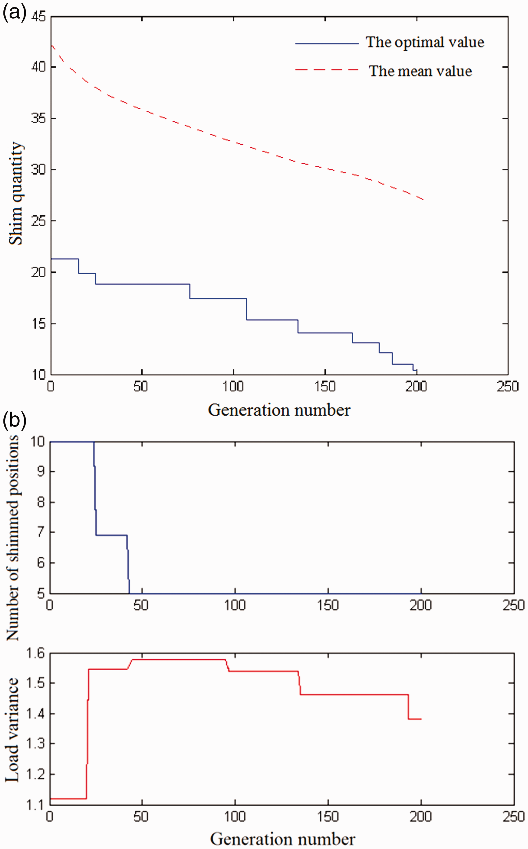
Change in the second preferential objective value for the HXD1D-type electric locomotive.

The optimisation results of load distribution, shim quantity and number of shimmed positions reveal that the new algorithm proposed in this paper can significantly improve manufacturing accuracy, reduce operation difficulty and save production cost in locomotive manufacturing process.

Conclusions

A new adjustment optimisation method for wheel (axle) load distribution is proposed in this paper, representing a breakthrough in locomotive load adjustment. Unlike traditional adjustment methods, which adjust the locomotive load by shimming the locomotive body and bogie separately, the new algorithm adjusts the wheel (axle) load distribution via the application of shimming on treads under entire locomotive conditions, with the vehicle body and the bogie considered as a single body prior to adjustment. As a result, problems of low efficiency, high costs and complex operation that characterise traditional two-step load adjustment methods are avoided.

The theoretical model for the entire locomotive load adjustment of a six-axle electric locomotive was established, with the tread measured model then obtained according to the theoretical model. Finally, the conversion model between primary shim quantity and tread shim quantity was established, thereby enabling the feasibility of simulating the primary shimming process by shimming on treads to be proven.

The proposed QAGA optimisation algorithm for entire locomotive load adjustment was adopted to simulate load adjustment tests using data for the HXD1D-type six-axle high-power electric locomotive. As shown in the application results, the new adjustment method successfully reduced the maximum deviation of the wheel (axle) load $\Delta F_{\max }$ to within the permissible limits of ±4% (±2%). Furthermore, the total shim quantity was reduced to only 15 mm and the number of shimmed supporting positions reduced from 10 to 5. The application results thus verified the efficiency, accuracy and feasibility of the proposed entire locomotive load adjustment method.