
Abstract
The research concerns analysis of transverse vibrations of power line transmission tower of variable cross section (changing on its length). Such constructions are subjected simultaneously to internal and external loads, which results in transverse and longitudinal vibrations. These vibrations are described by two partial differential equations of distributed parameters depending on two independent variables. If vibrations are small, the terms connecting equations of transverse and longitudinal vibrations can be neglected as infinitely small with respect to other quantities. Consequently, each vibration can be considered separately.
Introduction
The research aimed at analysis of transverse vibrations of power lines transmission tower of cross section changing along its length. Such constructions are subjected simultaneously to internal and external loads, which results in transverse and longitudinal vibrations. Considered vibrations can be described by two partial differential equations of distributed parameters depending on two independent variables. When the vibrations are small, the terms connecting equations of transverse and longitudinal vibrations can be neglected as infinitely small with respect to other quantities. Therefore, each vibration can be considered separately. Presented considerations concern transverse vibrations of power line pole while longitudinal vibrations will be the subject of a separate work.
The solution presented in the paper can be treated as a basis for development of a new method of studying vibrations of transmission towers. The scope of the carried out research covers:
formulation of the linear discrete–continuous model of the power line transmission tower, taking into account variable (in the function of the transmission tower length) geometry of the considered system, development of the assumed model mathematical description, formulation of the eigenproblem, providing solution of the initial-boundary problem taking into account the influence of external forces resulting in transverse vibrations of the considered system.
The structure of the paper is as follows. The next section concerns formulation of the linear discrete–continuous model of the power line transmission tower. Free vibrations are considered in the Free vibrations of the considered system section. In Formulation of eigenproblem section, eigenproblem is formulated. The initial-boundary problem is solved in the Solution of the initial-boundary problem section. Finally, conclusions and final remarks are given.
Linear discrete–continuous system model
Elaborated model associated with the power line transmission tower (of O24 type) consists of a single continuous element of distributed parameters (stiffness (EI)(x) and mass distribution (ρF)(x)) constrained at the bottom part. Functions (EI)(x) and (ρF)(x) are positive and continuous on the intervals. Under assumption that the changes in the values of these functions with respect to constants (ρ0F0) and (EI0) take place in small intervals; it is possible to describe these changes with the usage of the Dirac distribution.1–3 Such proceeding leads to the solution of the considered problem in the form of analytical formula. Obviously, this solution belongs to the space of generalized functions.
In Figure 1 there is presented discrete–continues model associated with the considered transmission tower O24 of overhead electrical power line. In the further considerations, the following notation was assumed: u(x, t) – relative displacement of the considered system cross section in the point x [m] at time t [s], ρ0 [kg/m3] – unit mass, F(x) [m2] – cross-section area, E [N/m2] – Young modulus, α0 [kg/m·s] – inner damping coefficient of the continuous element, I(x) [m4] – cross-sectional moment of inertia, H(x − a) and δ(x − a) [1/m] – Heaviside function and Dirac distribution concentrated at the point a, f(x, t) [N/m] – coordinate of the external force parallel to the pole axis, φ(x, ki, hi) [N/m] – coordinate of force associated with the massless constraints modelling interactions of electrical wires and the pole structure, ki [kg/s2], hi [kg/s] – stiffness and damping coefficients of the ith node, mi [kg] – mass concentrated at the point xi.
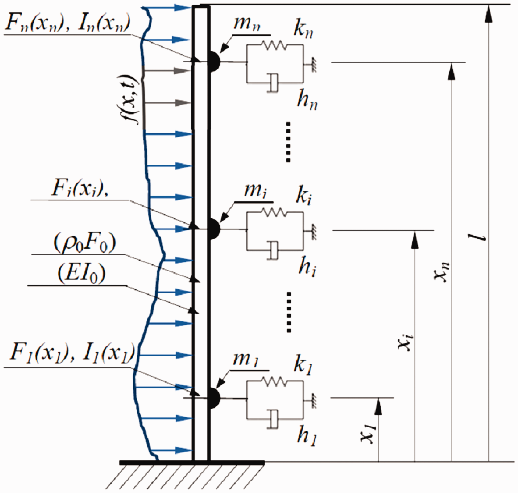
Model assumed for analysis of transverse vibrations of overhead electrical power line transmission tower.
Variability of cross section in the function of coordinate x.
Mass distribution in the function of coordinate x.
Distribution of cross-sectional moment of inertia in the function of coordinate x.
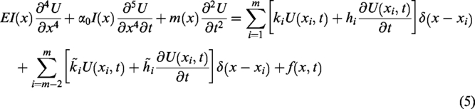
Influence of electrical cables on the considered structure was modelled by massless constraints arranged in short intervals along the pole length.4,5 In the carried out considerations it was assumed that formulated model mass equals mass of the real system. Model vibrations were described by partial differential equations of the fourth order with distributive coefficients
6
(p. 158). Solution of such equations belongs to the space of generalized functions, which means functions having distributive derivative at each point. The following assumptions concerning the pole structure were made:
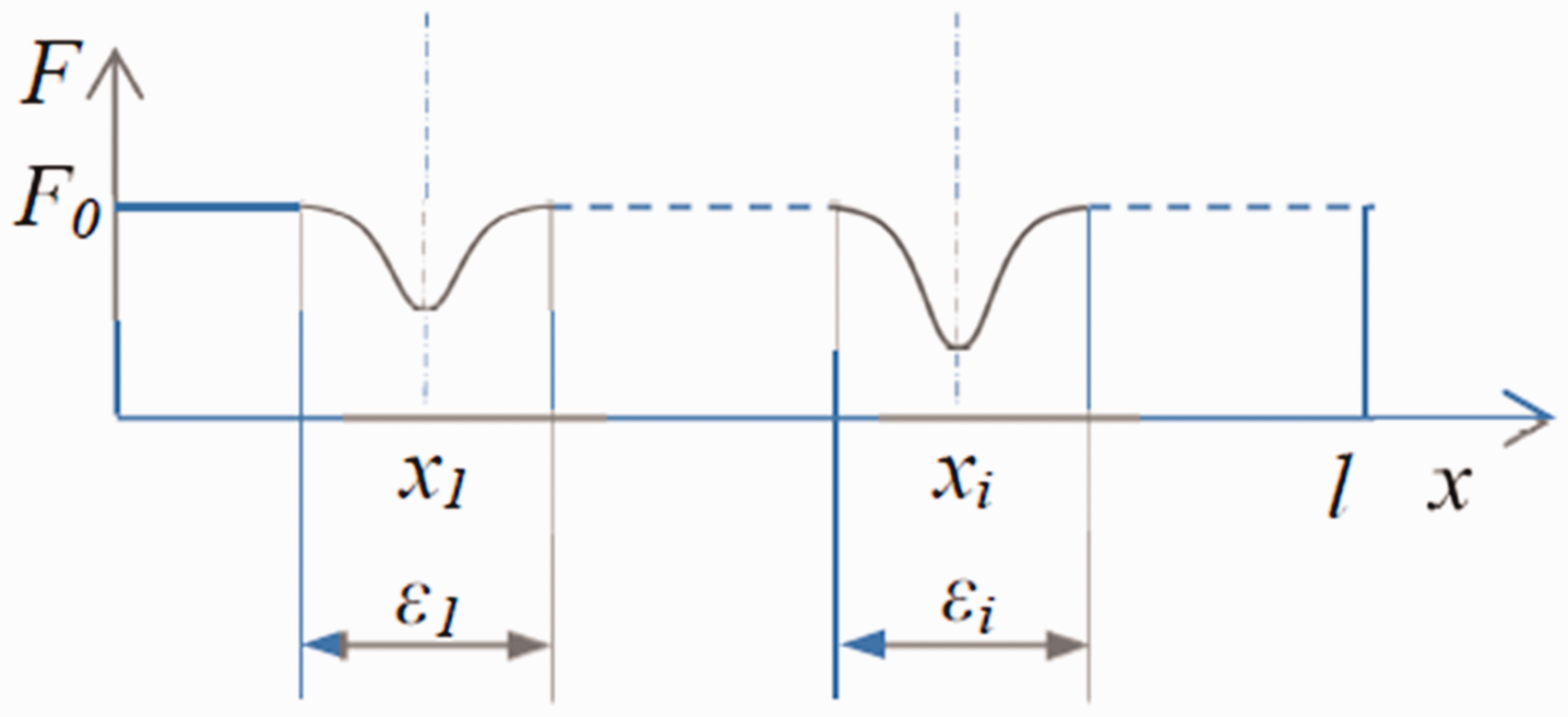
variability of pole cross section in the function of coordinate x (Figure 2)
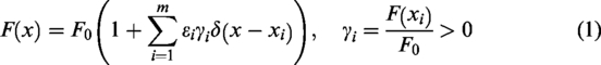
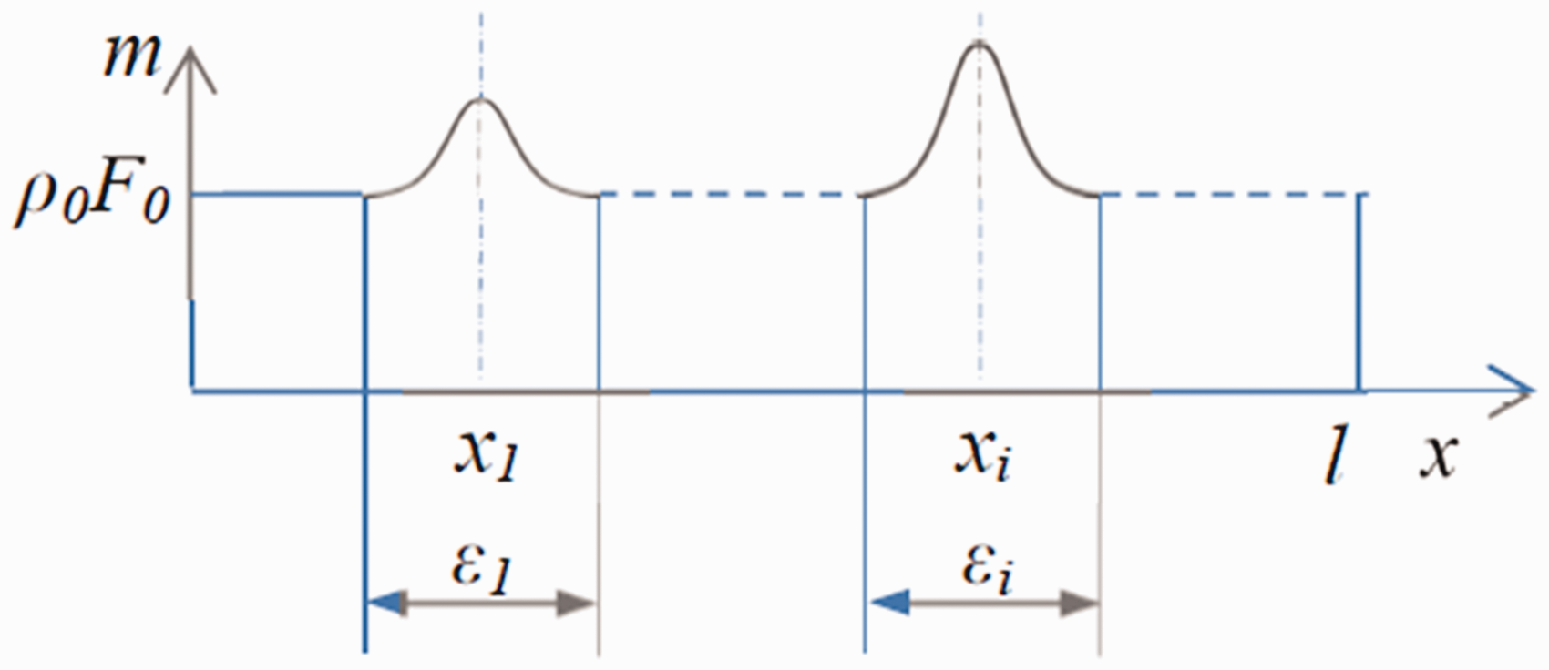
where: F0 [m2] = const, mass distribution (Figure 3)
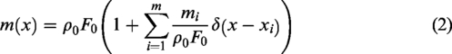
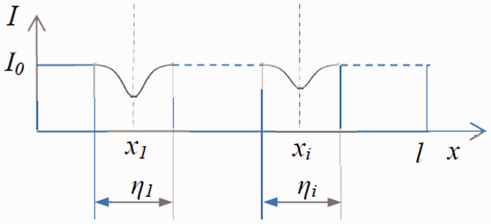
where: distribution of cross-sectional moment of inertia (Figure 4)
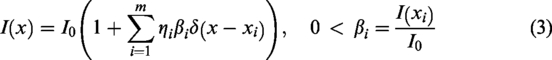
where: I0 [m4] = const, influence of electrical wires
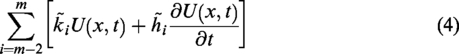
Using the notation


Due to the distributive coefficients in equation (5), solution of the initial-boundary problems (5) to (7) belongs to the class of generalized functions. In order to solve such a problem it is convenient to separate variables
9

For equation (8) it has to be assumed that
Due to the assumed forms of F(x), M(x), I(x) and ϕ(x) defined by formulas (1) to (4), equation (5) is linear. In the first step, the solution of free vibrations will be determined, in the following step – the solution of vibrations forced with the external force f(x, t).
Free vibrations of the considered system
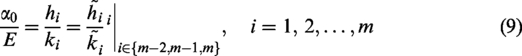
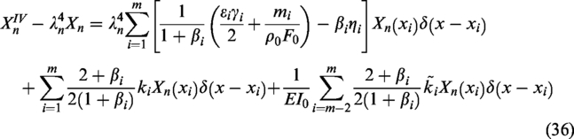
Inserting equation (8) into equations (5) and (6), taking into account equations (1) to (4) and (9)
10
(p. 90), having performed some standard operations, it can be written that
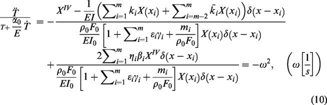

Relation (10) is equivalent to the equations

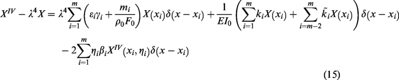
In equation (13), on the right side, there are components

In view of equation (14), equation (13) takes the form
For simplicity, in the further part of the paper,

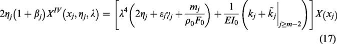
From equation (17) it follows that
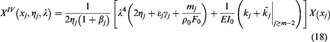
Having inserted equation (18) into equation (16) it was obtained
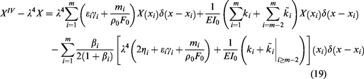
Parameters
Formulation of eigenproblem
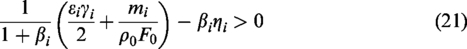
In order to find the solution of the eigenproblem, it is necessary to:
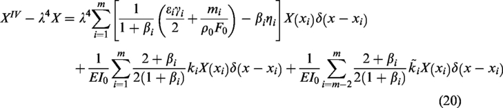
determine the set of generalized functions {X (x)} satisfying equation (20) with the boundary conditions (11), derive algebraic equation, the zeros of which are the eigenvalues λ of the eigenproblem problem being solved, derive orthogonality condition for elements of the set of functions satisfying equation (10), determine the solution of free vibrations of the considered system.
General solution of equation (11), in the class of generalized functions, is described by the equation
11
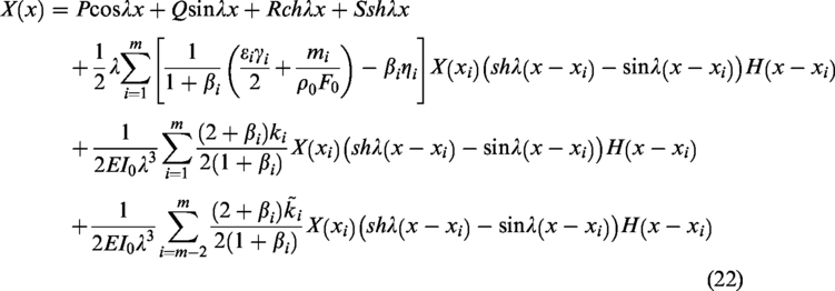
Due to the form of boundary conditions (11), from equation (22), the first three derivatives in the distributive sense should be calculated
12
(p. 76)
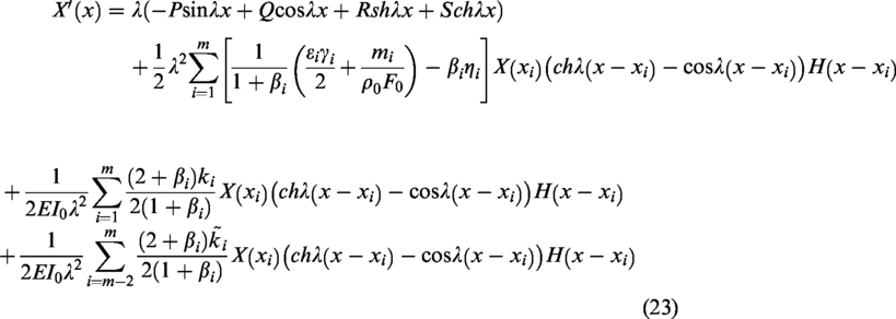

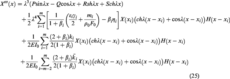
Constants P, Q, R and S can be determined from equations (22) to (25) and boundary conditions (11)

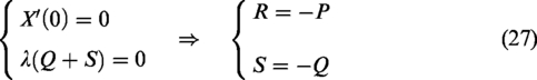
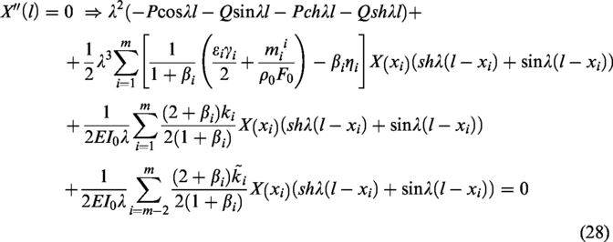
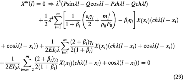
From equation (22), taking into account equations (26) and (27), it is possible to derive equations for calculating the remaining constants X(xi) at points xi (i = 1, 2, …, m)
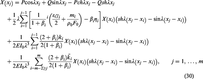
Set of equations (26) to (30) can be written in the matrix form

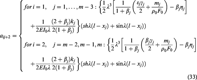
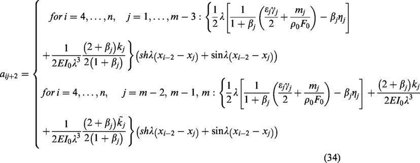
Matrix A(λ) has the following form
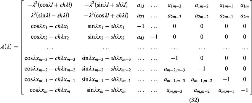
The set of equation (31) has nonzero solution when

Eigenvalues13,14 of the problems (20) and (11) form the solution of equation (35). Eigen values λn are positive and form an infinite series. Eigenvalues λn, correspond to functions {Xn(x)} forming the space of orthogonal functions.15,16 To prove the orthogonality condition, the method presented in Smirnov
10
(p. 102) was used. For Xn(x), with respect to each λn, the following differential equation can be written

Multiplying both sides of equation (20) by Xr(x) for n = s and equation (36) by Xs(x) for n = r, integrating in the interval [0, l], it was obtained that
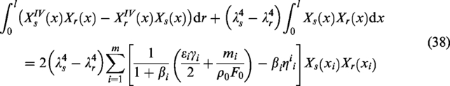
Integrating by parts the first component of equation (38) four times and taking into account boundary conditions, it was found out that this component equals zero. Therefore, equation (38) can be written as
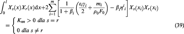
Functions describing free vibrations f(x, t)


Function (40) has to satisfy initial conditions. Therefore
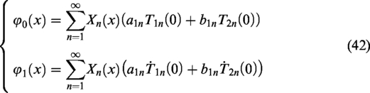
Since
Solution of the initial-boundary problem
Solution of the initial-boundary problems (5) to (7), under condition (14), was assumed in the following form
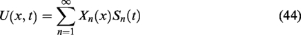
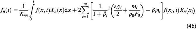
In order to formulate the second-order differential equation describing function Sn, equation (44) was inserted into equation (5), taking into account equation (14). Finally, both sides of the equation were multiplied by:

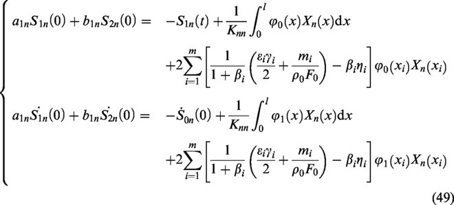
Particular solution of equation (45) can be written as

Taking into account the above considerations, solution of equation (44) can be described by the equation

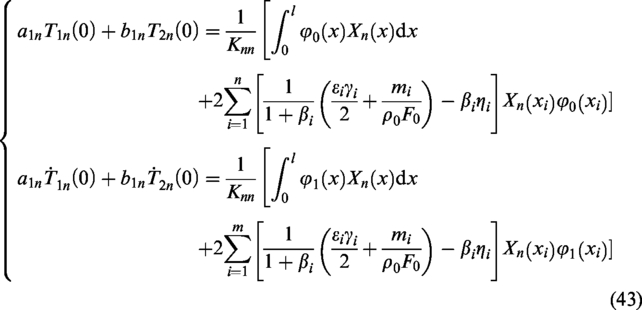
Constants a1
n
, b1
n
are determined from the set of equations
Since
Terms of series (20) and (48) should be treated as functions giving rise to the distributions 12 (p. 66), which means that series (20) and (48) are the series of distributions. These series are convergent in the distributive sense12,17 (p. 87). In practical applications, it is sufficient to take into account the first few terms of these series.
Numerical calculations were performed for the known model of the unilaterally restrained cantilever beam 18 of the following parameters: beam length: 0.8 [m], material density: 7820 [kg/m3], the Young’s modulus: 210,000 [MPa], beam cross section: 0.0004 [m2], geometrical moment of inertia: 1.333333 10−8 [m4]. The calculations aimed at determining the influence of supporting linear spring on the beam dynamic behaviour. In the course of analysis, the spring stiffness coefficient was changed in the range of 0–500,000 [N/m] with the step of 50,000 [N/m]. The impact of spring was modeled as a local discontinuity (concentrated force), the location of which was changed in the range of 0 [m] to 0.8 [m] with the step of 0.05 [m]. Dependence of the first wave number calculated for the entire system as a function of force location and value of spring modulus of elasticity is shown in the Figure 5.
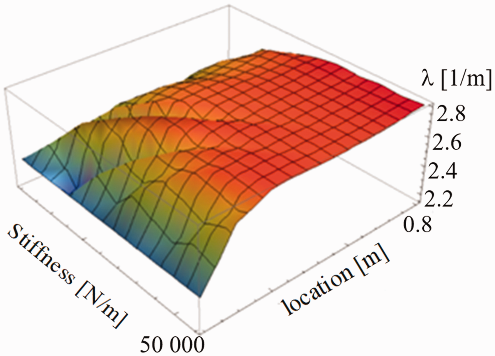
The first wave number of the considered cantilever beam calculated in the function of force location and value of spring modulus of elasticity.
Roots of equation (32) were determined numerically, with the application of direct root finding methods and LU decomposition.19,20 Due to low efficiency of gradient methods and resulting necessity of searching for the solution in the consecutive intervals, the task of root finding is not trivial.
Conclusions and final remarks
In the carried out research the discrete–continuous model of the truss power pole was formulated. In the considered partial differential equations describing vibrations of power pole, the changes in the system parameters were modelled with the use of the products of the second order derivatives at points xi and the Dirac distribution. Difficulties with application of the proposed description of the system vibrations result from the fact that the first derivatives are discontinuous at xi and, therefore, products of derivatives are indeterminate. On the other hand, the Dirac functions occurring in the equations describing the system vibration result from the assumed model. To avoid multiplication of Dirac functions, in the carried out research it was proposed to approximate second derivatives at the points xi by arithmetical means of their values in the neighbouring points xi − ηi, xi + ηi. Such proceeding allows for elimination of products of distributions from the considered equations. As the result the proposed model can be solved with the application of standard methods.
In the paper, the eigenproblem was formulated and solved. The authors presented differential equation on the basis of which eigenfunctions were determined. In the further part of the paper othogonality of eigenfunctions was proved and, taking into account external forces exciting transverse vibrations of the considered system, the initial-boundary problem was solved. Obtained solution has the form of infinite series.
For properly selected geometrical parameters of the continuous component, equations describing eigenfunctions and eigenvalues can be significantly simplified. Local abrupt changes in the geometrical properties of the system (power pole) affect only the first few eigenvalues, while the other eigenvalues remain almost unchanged with respect to the eigenvalues of the system of constant cross section.
Carried out analysis of power pole transverse vibrations can be extended to any truss systems. The analysis is based on the formulation of the discrete-continuous model of the considered truss system, i.e. cross section determining, selection of linear parameters and massless constraints. These constraints have to correspond to local changes in stiffness of the truss system. Selection of parameters for discrete-continuous model will be the subject of a separate work.
Footnotes
Declaration of conflicting interests
The author(s) declared no potential conflicts of interest with respect to the research, authorship, and/or publication of this article.
Funding
The author(s) received no financial support for the research, authorship, and/or publication of this article.