Sage Journals: Discover world-class research

Abstract

Room resonances create dramatic fluctuations in the distribution of sound pressure throughout the listening region of a room. Previous studies indicate that the addition of sound absorbing material decreases room resonances and shifts its modal characteristics. The present study proposes an approach which qualifies the effects that the additional absorption in a listening room may have on the sound fields and the frequency responses. Finite element analysis was employed for modelling the low-frequency responses of a room. The study analyses frequency responses at various listening positions involving different amounts and different placement of sound absorbents on room surfaces by observing standard deviation for linearity across a chosen frequency range. Two-dimensional sound field plots at listening height were also used to examine the spatial changes of room resonances caused by the additional absorption. The present study applied a modified statistical approach to evaluate both the sound field and the frequency responses of a room. The results were then applied to re-evaluate the effects of the absorbers location on the listening region through the proposed approach.

Keywords

Sound field absorption frequency responses

Introduction

Spaces dominated by low frequencies have been studied in wave theory since 1940.^1,2 A number of studies focused on room acoustics,³ sound insulations,^4–6 and boundary conditions.⁷ With the emergence of professional recording and digital audio technology, the study of small critical listening environments has recently gained prominence. The advancements in audio technology and rising popularity of small rooms for critical listening have made small room acoustics a popular area of research over the past several years.⁸ Unlike large performance spaces or rooms with complicated shape which exhibit increased modal density or lower Schroeder/transition frequency,^9,10 standing waves become a problem in lower frequencies as the size of a room decreases. Optimum room ratios^11–15 and room modal distributions^16,17 were previously researched in several studies.

A number of studies, some of which date as far back as the 1940s,^1,2 used modal spacing as the criteria for low-frequency performance of a room. These theories suggest that the frequency response within a room will be increasingly regular the more evenly the modes are spaced across the frequency spectrum. The first iteration of the theory attempted to minimize the average spacing between each mode.¹ It was later determined that the average mode spacing was not a good indicator of modal performance.¹⁴ The ratio calculated by Bolt¹ did not consider weighting between axial and the weaker tangential and oblique modes, and due to this, the stronger axial modes dominated room configuration. Future studies built on the foundation set by Bolt for low-frequency optimization.

Room modes cause unwanted effects for sound reproduction in listening rooms.¹⁸ Solutions to these problems vary from simple loudspeaker/listener positioning, and complex signal processing,^19–21 to architectural design. Toole²² reviewed some of these solutions and concluded that current assumptions in the design of large performance spaces may not be valid as spaces turn smaller and more acoustically absorptive. Strong modal behaviour of space can be observed at frequencies below approximately 300 Hz. Currently, there is a general lack of methods towards identifying this transition frequency.

Recently, modal decay thresholds have shown to be a more promising tool for the evaluation of audible artifacts in listening environments at low frequencies.^21,23–26 Modal decay perceptual thresholds can help reduce the complexity of a modal control system or design. There are some studies that address the frequency and level dependency of perceptual thresholds as the functions of modal decay.²⁶ A strong correlation has been identified²⁵ between the perceived improvement in the reproduction quality and the decay time of low-frequency energy in a room. Subjective tests also show that room aspect ratios affect the perception of modal distribution.²⁴ However, as of yet, a simple objective method evaluating architectural design or room shape based on the simulated or measured frequency responses of a room has not been attempted.

Often subject to debate is the alteration of room geometry in order to solve modal problems. Splaying the walls or adjusting the acoustic mass of a room through surface undulations or depressions will undoubtedly change mode shapes and shift modal frequencies, possibly improving the sound field. However, these alterations make the low-frequency performance much more difficult to predict when compared to the performance of a rectangular space.^27,28 Changes to the geometry of a room do not eliminate modal effects on the sound field and listening responses: they simply make them harder to predict.²⁹ When attempting to predict modal behaviour of the space, it should be noted that non-rectangular spaces do not follow the simple formulation of eigen-frequencies that rectangular spaces do.

Papadopoulos²⁸ recently investigated the modification of rooms with rectangular geometry in order to produce smoother distribution of sound energy in the low-frequency range. The study observed regional depressions and indentations in a room that change the modal response. The study proposed that the addition or removal of acoustic mass (air) at specific points within a room would shift and damp modal frequencies and create a more pleasant listening environment. By using this methodology, Papadopoulos²⁸ was able to take non-ideal rectangular room ratios with degenerate modes and use geometric irregularities in the model to improve the low-frequency performance. Geometric modifications were made by computer optimization algorithms that sought out the optimum conditions that produced as closely linear frequency response of the room as possible. The results of the research showed that the algorithm was able to make changes to the sound field. Most notably, the algorithm adjusted the modal frequencies from a degenerate mode condition to an evenly spaced mode condition. The algorithm was also able to slightly damp the modes so that the maximum and minimum sound pressure levels were not as disparate. The results showed that the standard deviation of the frequency response for the room was reduced from 3.3 decibels to 2.8 decibels, a noteworthy improvement.²⁸ However, the nature of the modifications proved to be impractical and would have been be difficult to apply to actual construction.

Previous studies also investigated the effects related to the addition of room elements to a low-frequency finite element model. Adding elements such as beams, columns, and furniture to a room and then analysing the effects of those elements on the frequency responses and the low-frequency sound field helped better understand the actual low-frequency responses. Eda et al.³⁰ devised a finite element room model and ran 29 iterations of the model, each containing one different room element. The study concluded that the addition of columns, beams and furniture to a perfectly rectangular room helped create smoother frequency response at listening positions in the room, though of varying performance degrees. Even if the standard deviation of the frequency response at the main listening position was improved, other nearby positions could have degraded significantly. Therefore, in order to determine the overall acoustic effect of the added elements,³⁰ an analysis of several positions throughout the room is required. The study of effects that the addition of practical items such as furniture and columns has on the low-frequency sound field is a much needed step towards better understanding of the actual low-frequency performance in small rooms. However, the flatness characteristic, related to both frequency and space ( $S D_{f, s}$ ), is calculated based on multiple standard deviations of frequency (SD_f) and space (SD_s). $S D_{f, s}$ can be lower if either SD_s or SD_f are lower. Therefore, this approach may not reflect the unevenness of the frequency variation spatial distribution over the subject space/domain. The present study proposes the evaluation of the sound field that is based on the average SD_f over the space, and the visualization of SD_f. Statistical analysis and standard deviations are also applied with regard to subwoofer/source optimization in a room.³¹ Due to the popularity of wall-mounted absorption in listening rooms, the authors hope that this study will add to previous research and help provide a more complete understanding of the effects of various elements on the low-frequency performance in space.

Numerical modelling

Room model

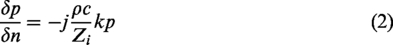
The finite element analysis (FEA) software package, COMSOL Multiphysics, was used to model the sound propagation. The finite element computation solves the inhomogeneous wave equation as follows

\nabla^{2} p + k^{2} p = q

(1)

where p and k represent the complex acoustic pressure and the wave number of the sound, respectively; q denotes the source strength density of the excitation; and

\nabla^{2}

is the Laplacian operator over a specified domain with Neumann boundary conditions. Although the study employs commercial software, it is only used to generate frequency responses of a room in order to evaluate the proposed method and the absorbers placement. Frequency responses can also be obtained by other methods and measurements.

The room model closely resembles a realistically sized small room to which the acoustic treatments are to be applied. Louden¹¹ widely appreciated room ratio of 1:1.4:1.9 was used in order to avoid degenerate modes. Considering the typical ceiling height of 3 m, the study sized the room 4.2 m by 5.7 m by 3 m. Based on its shape, the room volume stands at approximately 72 m³ with the Schroeder frequency of over 200 Hz assuming the average absorption coefficient of less than 0.22. Figure 1 displays the model geometry.

Figure 1.

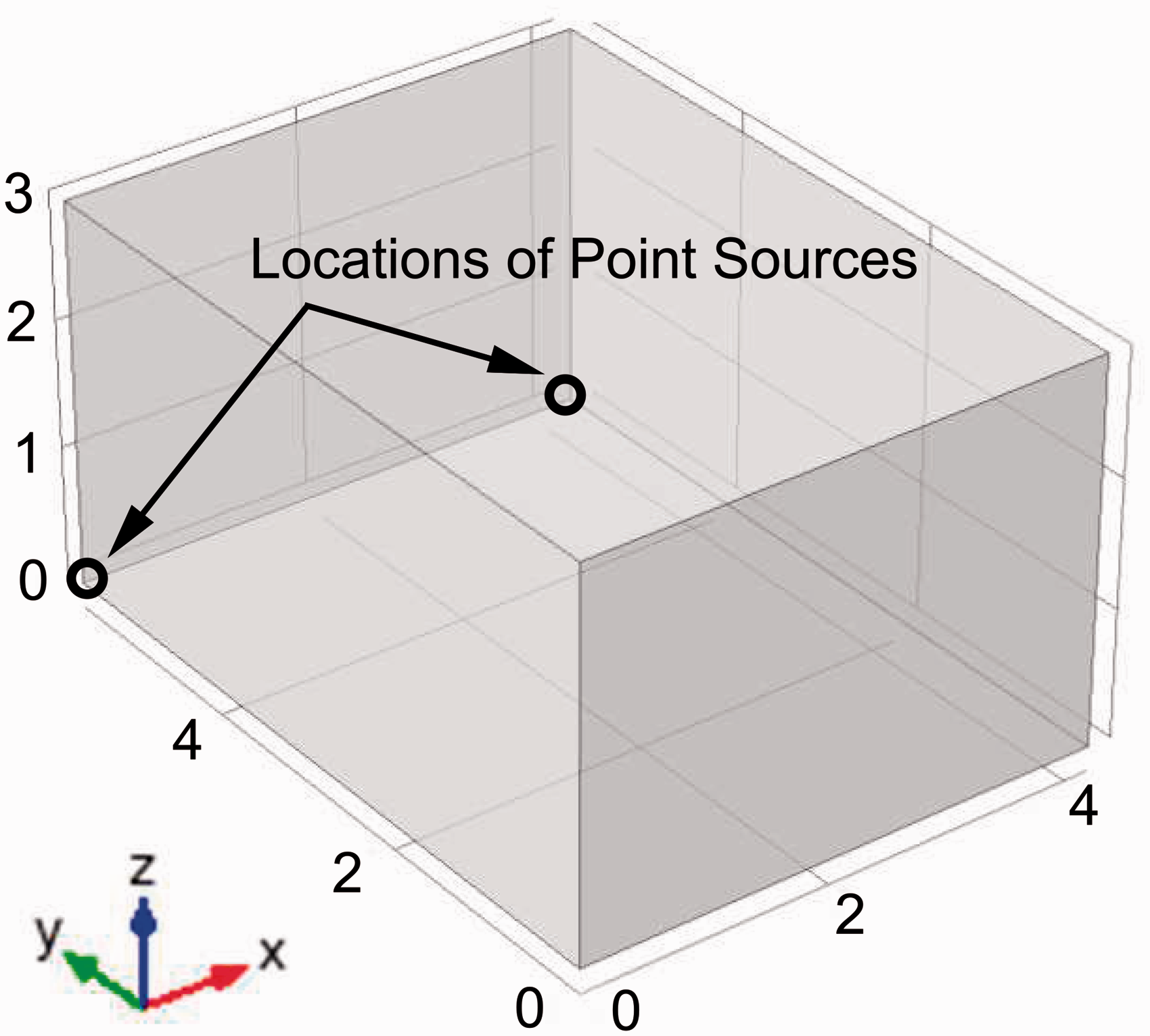
Room geometry and coordinate system (in meters).

Boundary conditions and mesh size

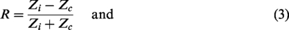
In order to obtain the desired results, the impedance boundary conditions on all surfaces were set as follows

\frac{δ p}{δ n} = - j \frac{ρ c}{Z_{i}} k p

(2)

where

j = \sqrt{- 1}

; n denotes the outgoing normal of the surface; ρ and c stand for the density of sound and the sound speed in the air, respectively. Z_i represents the acoustic impedance on the i^th surface. Sound absorption coefficients are based on Z_i,³² where the reflection coefficient R and the normal incidence absorption coefficient are calculated as follows

R = \frac{Z_{i} - Z_{c}}{Z_{i} + Z_{c}} and

(3)

α = 1 - | R |^{2}

(4)

with Z_c being the typical impedance of air. The acoustic impedance corresponding to the normal incidence absorption coefficient α = 0.10 was allocated to all six surfaces of the initial rectangular model. The value α = 0.10 relates to the approximate measured low-frequency absorption of the standard wood frame with plaster board wall.

The mesh size is determined by the wavelength of the highest frequency of interest. The largest acceptable mesh size is 0.2144 m, or one eighth of the wavelength at 200 Hz. Constructing a free tetrahedral-shaped mesh with the largest acceptable mesh length inside the 72 m³ volume, generated a mesh with about 127,000 elements.

Sound source and model verification

A pair of sound sources was added to the model in order to excite the room with a time-harmonic source. The point sources were located at two corners as shown in Figure 1, in order to avoid the nodal lines of any acoustic mode in the rectangular enclosure. Each point source radiated at a constant power of 0.1 W with even power distribution from 20 to 200 Hz. The two sources were used to mimic the sound reinforcement system in a small room. It may be expected that the two in-phase sources at symmetrical locations will suppress asymmetrical model responses; however, in terms of frequency responses, such positioning may be the worse scenario. Nevertheless, the study used the proposed approach focusing on the optimization of the absorption materials placement.

In order to verify that the initial model accurately calculated eigen-frequencies, the FEA model results were compared to the frequencies calculated by an analytical model with acoustically rigid walls. The largest difference between the initial 20 modes amounted to 0.03%. The result verified the accuracy of the model for future iterations.

Sound absorption modelling

With the initial model verified for accuracy, the parameters for modelling acoustically absorbing devices were then added. Current FEA model uses Delaney and Bazley model³³ to estimate sound absorbing properties (i.e. complex sound speed and complex density) of porous materials. The model may have shown some deviations at low frequencies; however, the absorption is low at these frequencies and may not be relevant to the objective of this study which is to examine the proposed method. Based on the results of the previous studies,³⁴ the average value for a standard acoustic absorbing fibreglass was determined to be 20,000 Pa $\cdot$ s/m².

In order to account for the addition of absorptive material to the initial model, volume domains were added to the FEA model to simulate typical treatment locations. In total, 34 absorptive devices were added to the model at pre-set locations on walls and ceiling. Thirty panels were the typical 0.6 m by 1.2 m by 0.1 m thick fibreglass absorbers on the rigid boundary and were distributed evenly along each wall with the bottom edge 1 m above the floor. Figure 2 provides a view from the top of the room and also labels all absorber volume domains by number. The remaining four treatments were corner absorbers (domains 2, 8, 29, and 30 in Figure 2). The corner absorbers had a radius of 0.3 m and extended vertically downward from the ceiling to 0.3 m from the ground in each of the four corners (a total height of 2.7 m). The location of the two point sources is marked by the two circles.

Figure 2.

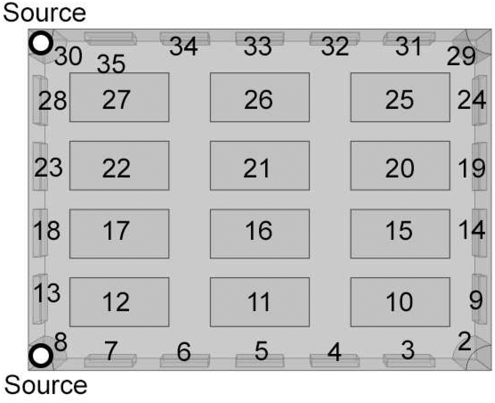
Absorber domain locations.

The speed of sound in the absorbing material previously described whose flow resistance is 20,000 Pa $\cdot$ s/m², was determined to stand at 64.36 m/s at 200 Hz. The smallest acceptable mesh size inside the absorbing material was 0.04023 m – a much finer mesh than at standard air conditions. When the final mesh was compiled, the model contained over 255,000 elements with all 34 absorber domains active.

The standard acoustic absorbing fibreglass materials with 0.1 m thickness may have limited sound absorption at low frequencies. Figure 3 shows the normal incident sound absorption coefficients that are higher than 0.2 at frequency above 100 Hz – values commonly featured in small listening spaces. In order to control the low-frequency sound, porous absorbers can be used though this may not be a good strategy. This study, however, aims at re-evaluating the effects of the absorbers location on the listening region through the proposed approach.

Figure 3.

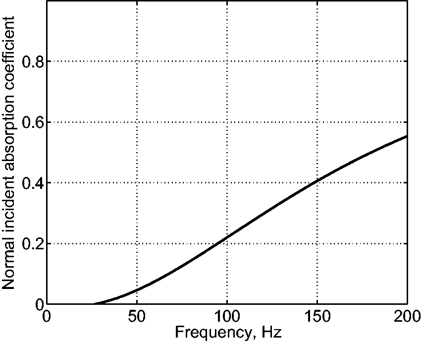
Normal incident sound absorption coefficients of the absorptive material (20,000 ${Pa·s/m}^{2}$ ), thickness 0.1 m.

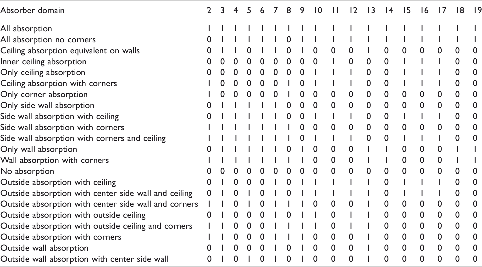
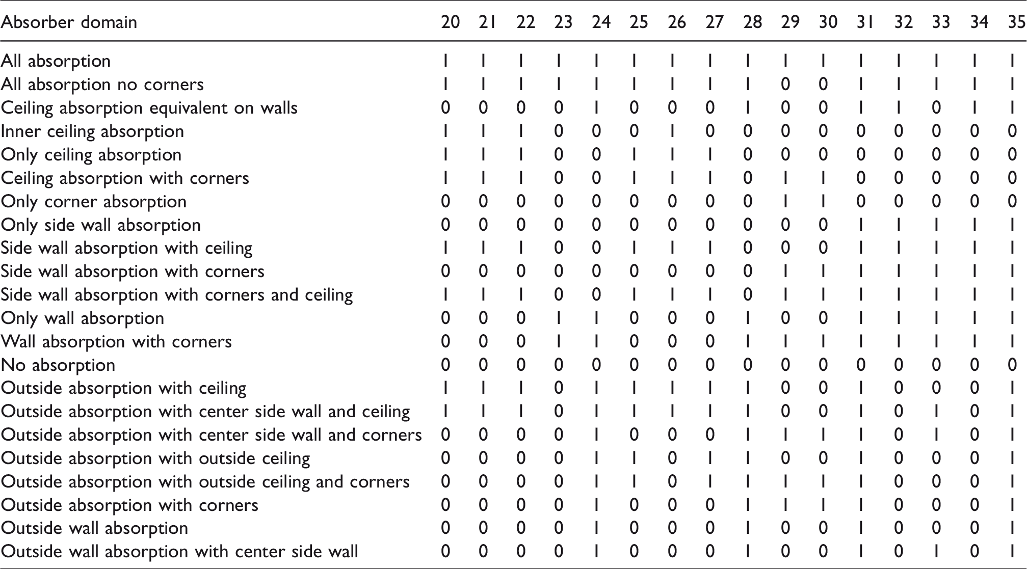
In order to test the effects of absorption within the room, several different absorption configurations were tested. Modal responses are highly sensitive to the corresponding shape of the model room. Pressure sensitive absorbers (e.g. panel and Helmholtz) are optimally placed at high pressure locations, whereas the optimal placement of porous absorbers is at locations with high particle velocity. This study examines frequency responses at pre-set locations in the room some of which may not be optimal for porous absorbers. Hence, they are potential locations for the placement of absorbers. Tables 1 and 2 describe absorber status for each analysed room absorption configuration. Absorber domains from Figure 2 are labelled accordingly starting with row 2 through 35 (domain 1 is the large air volume of the listening space). First column contains the names of absorption configurations, whereas the second column provides numerical configuration descriptions. Value 1 denotes that a particular acoustic domain is active as an absorber device, whereas value 0 denotes that the domain is inactive and has typical air properties.

Table 1.

Absorption configurations for domains 2 to 19.

Absorber domain	2	3	4	5	6	7	8	9	10	11	12	13	14	15	16	17	18	19
All absorption	1	1	1	1	1	1	1	1	1	1	1	1	1	1	1	1	1	1
All absorption no corners	0	1	1	1	1	1	0	1	1	1	1	1	1	1	1	1	1	1
Ceiling absorption equivalent on walls	0	1	1	0	1	1	0	1	0	0	0	1	0	0	0	0	0	0
Inner ceiling absorption	0	0	0	0	0	0	0	0	0	1	0	0	0	1	1	1	0	0
Only ceiling absorption	0	0	0	0	0	0	0	0	1	1	1	0	0	1	1	1	0	0
Ceiling absorption with corners	1	0	0	0	0	0	1	0	1	1	1	0	0	1	1	1	0	0
Only corner absorption	1	0	0	0	0	0	1	0	0	0	0	0	0	0	0	0	0	0
Only side wall absorption	0	1	1	1	1	1	0	0	0	0	0	0	0	0	0	0	0	0
Side wall absorption with ceiling	0	1	1	1	1	1	0	0	1	1	1	0	0	1	1	1	0	0
Side wall absorption with corners	1	1	1	1	1	1	1	0	0	0	0	0	0	0	0	0	0	0
Side wall absorption with corners and ceiling	1	1	1	1	1	1	1	0	1	1	1	0	0	1	1	1	0	0
Only wall absorption	0	1	1	1	1	1	0	1	0	0	0	1	1	0	0	0	1	1
Wall absorption with corners	1	1	1	1	1	1	1	1	0	0	0	1	1	0	0	0	1	1
No absorption	0	0	0	0	0	0	0	0	0	0	0	0	0	0	0	0	0	0
Outside absorption with ceiling	0	1	0	0	0	1	0	1	1	1	1	1	0	1	1	1	0	0
Outside absorption with center side wall and ceiling	0	1	0	1	0	1	0	1	1	1	1	1	0	1	1	1	0	0
Outside absorption with center side wall and corners	1	1	0	1	0	1	1	1	0	0	0	1	0	0	0	0	0	0
Outside absorption with outside ceiling	0	1	0	0	0	1	0	1	1	0	1	1	0	0	0	0	0	0
Outside absorption with outside ceiling and corners	1	1	0	0	0	1	1	1	1	0	1	1	0	0	0	0	0	0
Outside absorption with corners	1	1	0	0	0	1	1	1	0	0	0	1	0	0	0	0	0	0
Outside wall absorption	0	1	0	0	0	1	0	1	0	0	0	1	0	0	0	0	0	0
Outside wall absorption with center side wall	0	1	0	1	0	1	0	1	0	0	0	1	0	0	0	0	0	0

Table 2.

Absorption configurations for domains 20 to 35.

Absorber domain	20	21	22	23	24	25	26	27	28	29	30	31	32	33	34	35
All absorption	1	1	1	1	1	1	1	1	1	1	1	1	1	1	1	1
All absorption no corners	1	1	1	1	1	1	1	1	1	0	0	1	1	1	1	1
Ceiling absorption equivalent on walls	0	0	0	0	1	0	0	0	1	0	0	1	1	0	1	1
Inner ceiling absorption	1	1	1	0	0	0	1	0	0	0	0	0	0	0	0	0
Only ceiling absorption	1	1	1	0	0	1	1	1	0	0	0	0	0	0	0	0
Ceiling absorption with corners	1	1	1	0	0	1	1	1	0	1	1	0	0	0	0	0
Only corner absorption	0	0	0	0	0	0	0	0	0	1	1	0	0	0	0	0
Only side wall absorption	0	0	0	0	0	0	0	0	0	0	0	1	1	1	1	1
Side wall absorption with ceiling	1	1	1	0	0	1	1	1	0	0	0	1	1	1	1	1
Side wall absorption with corners	0	0	0	0	0	0	0	0	0	1	1	1	1	1	1	1
Side wall absorption with corners and ceiling	1	1	1	0	0	1	1	1	0	1	1	1	1	1	1	1
Only wall absorption	0	0	0	1	1	0	0	0	1	0	0	1	1	1	1	1
Wall absorption with corners	0	0	0	1	1	0	0	0	1	1	1	1	1	1	1	1
No absorption	0	0	0	0	0	0	0	0	0	0	0	0	0	0	0	0
Outside absorption with ceiling	1	1	1	0	1	1	1	1	1	0	0	1	0	0	0	1
Outside absorption with center side wall and ceiling	1	1	1	0	1	1	1	1	1	0	0	1	0	1	0	1
Outside absorption with center side wall and corners	0	0	0	0	1	0	0	0	1	1	1	1	0	1	0	1
Outside absorption with outside ceiling	0	0	0	0	1	1	0	1	1	0	0	1	0	0	0	1
Outside absorption with outside ceiling and corners	0	0	0	0	1	1	0	1	1	1	1	1	0	0	0	1
Outside absorption with corners	0	0	0	0	1	0	0	0	1	1	1	1	0	0	0	1
Outside wall absorption	0	0	0	0	1	0	0	0	1	0	0	1	0	0	0	1
Outside wall absorption with center side wall	0	0	0	0	1	0	0	0	1	0	0	1	0	1	0	1

Analysis methods

Rooms were evaluated based on the frequency responses of listening positions. The FEA model defined a dense grid of evaluation points. The grid was placed 1.2 m above the floor (i.e. the average ear height for a seated listener). For each grid point, FEA calculated the level of sound pressure at frequency intervals of 2 Hz. Thereafter, an SPL plot versus frequency was made at each point in the grid area. The plots are considered to be the frequency response at each position.

Previous studies accept the standard deviation of mode spacing as a factor of the acoustic quality of low-frequency performance in a room.^1,30 Rooms with higher performance had lower standard deviation values indicating that the modes were more evenly separated in space through other modal frequency ranges. The standard deviation value of frequency response would also be at a higher value for rooms with close modes or with further spread modes. The present study evaluates the absorber placement based on the regularity of the frequency responses across the listening space. The aim is to reduce the frequency distortion; hence, the optimization involves minimizing standard deviations.

The linear standard deviation from the mean was used to determine the linearity of the frequency response plot. Eda et al.³⁰ developed a methodology that analyses the spaces for low-frequency performance. They used the standard deviation of point frequency responses and also compared the two-dimensional plots showing the standard deviation at all points. This study used a modified methodology to analyse the frequency responses of rooms with and without absorption. Data grid was plotted as the 2D standard deviation of frequency responses over the listening area. The listening region evaluated in this study ranges from 2.5 m to 5 m along the length of the room and is centered between 1.1 m and 3.1 m along the width. This particular region was chosen based on previous iterations of the whole room standard deviation sound field to define the best listening region and also to determine the region that would best describe and isolate the effect of the added absorption. Figure 4 depicts the location of the grid plane within the room. In this study, the standard deviation data were also averaged over the entire listening region to acquire a performance metric for the whole space.

Figure 4.

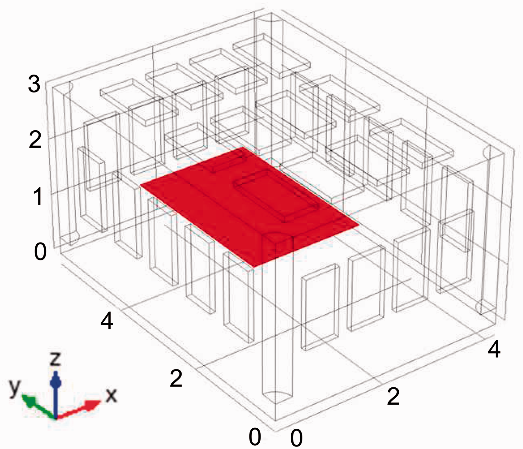
Location of the analysed grid plane in the room (the evaluated listening region is marked in red).

The results obtained in this research imply that human subjective response will be more positive when the frequency response at a listening position is more linear. When frequency responses become more linear due to the addition of absorbents, it assumes a decrease in the Q-value of the modes. According to the research of Avis et al.,²³ this reduction in the standard deviation leads to a decrease in the resonance decay time and improves subjective perception of low frequencies in the space.

As concluded in a study by Eda et al.,³⁰ the analysis of one or even several frequency responses is not enough to provide an accurate description of the overall sound field quality in a room. Since the goal of this research is to improve the frequency response across many positions in a room rather than optimize just one specific listening position, spatial distribution of standard deviations was analysed across the whole dense grid of data points. The data obtained revealed that while some listening positions improved, others degraded, and vice versa. Only when the spatial average of the standard deviation of the frequency responses improved as a whole did the acoustic quality of the listening area of the room improve as well. The effect of the addition of absorption to certain areas of the room was also observed in relation to the spatial averaging plots. The study hypothesised that absorption in specific areas of the room will smoothen out the responses in the predictable areas of the sound field and aimed to quantify such prediction more accurately. Spatial plots and spatial averages were used to quantify the effect of the added absorption in the space.

Results and discussions

Twenty-two iterations in total were analysed for the low-frequency performance based on the standard deviation metrics as described in the analysis methods section. The sub-sections below detail the acquired modelling results and analyse the changes in the frequency response and the sound field of the listening region caused by the addition of absorptive material.

Comparison of the average standard deviation

The first method of analysis employed in this study compared the standard deviation averaged over the listening area, $\bar{S D}$ (dB), for each absorption configuration in order to quantify the overall performance of the listening region for each absorption configuration. In this way, the uniformity of the sound fields and frequency responses could be evaluated. Table 3 compares the calculated average standard deviation of all absorption configurations based on the amount of absorption present within each configuration.

Table 3.

Analysis of the average standard deviation of the listening region.

Absorption configuration	TotalAbsorptionArea (m²)	$\bar{S D}$ (dB)
No absorption	0.00	6.13
Only corner absorption	5.17	6.12
Inner ceiling absorption	5.95	5.85
Outside wall absorption	5.95	5.98
Only side wall absorption	7.43	5.94
Outside wall absorption with center side wall	7.43	5.94
Ceiling absorption equivalent on walls	8.92	5.96
Only ceiling absorption	8.92	5.80
Outside absorption with outside ceiling	8.92	5.99
Outside absorption with corners	11.12	5.97
Side wall absorption with corners	12.60	5.98
Outside absorption with center side wall and corners	12.60	5.92
Only wall absorption	13.38	5.89
Ceiling absorption with corners	14.09	5.88
Outside absorption with outside ceiling and corners	14.09	5.92
Outside absorption with ceiling	14.86	5.74
Side wall absorption with ceiling	16.35	5.62
Outside absorption with center side wall and ceiling	16.35	5.65
Wall absorption with corners	18.55	5.84
Side wall absorption with corners and ceiling	21.52	5.69
All absorption no corners	22.30	5.59
All absorption	27.47	5.64

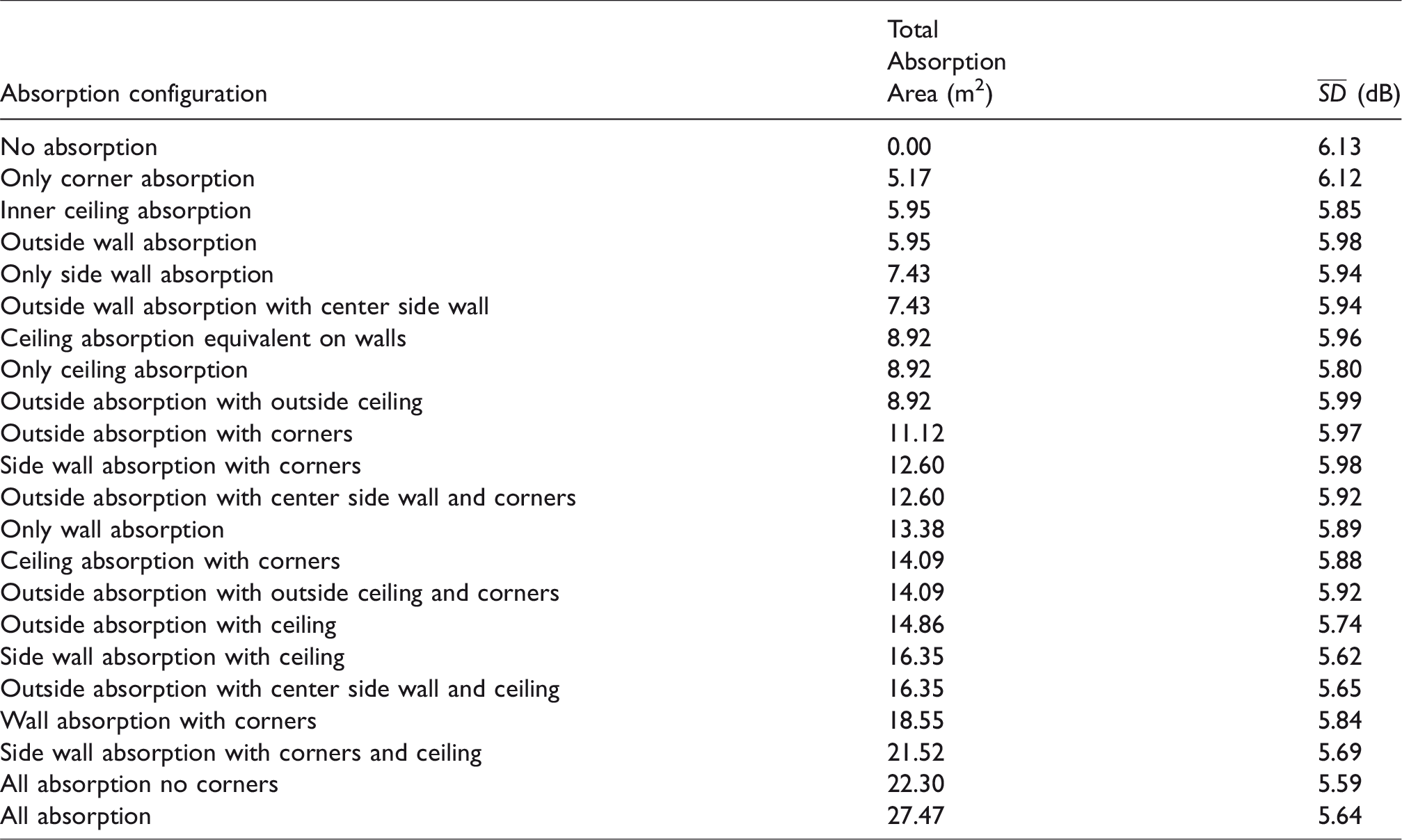
Figure 5 presents the $\bar{S D}$ trend against total active absorption areas in the space. Although the data in this series is not perfectly linear, a general trend could be derived from the results which the average standard deviation decreases approximately to 0.02 dB/m². The addition of absorption reduced the average standard deviation in the listening region. The range of the results spans 0.54 dB. According to the results and conclusions of a study by Eda et al.,³⁰ such change in the average standard deviation for a listening region may be considered as significant. However, further study is needed to verify the significance of the change subjectively. The modification in this study is also limited by the low absorption of the porous panel absorber at low frequency. A wider range of standard deviations may also be obtained through other types of sound absorbers or other room treatments.

Figure 5.

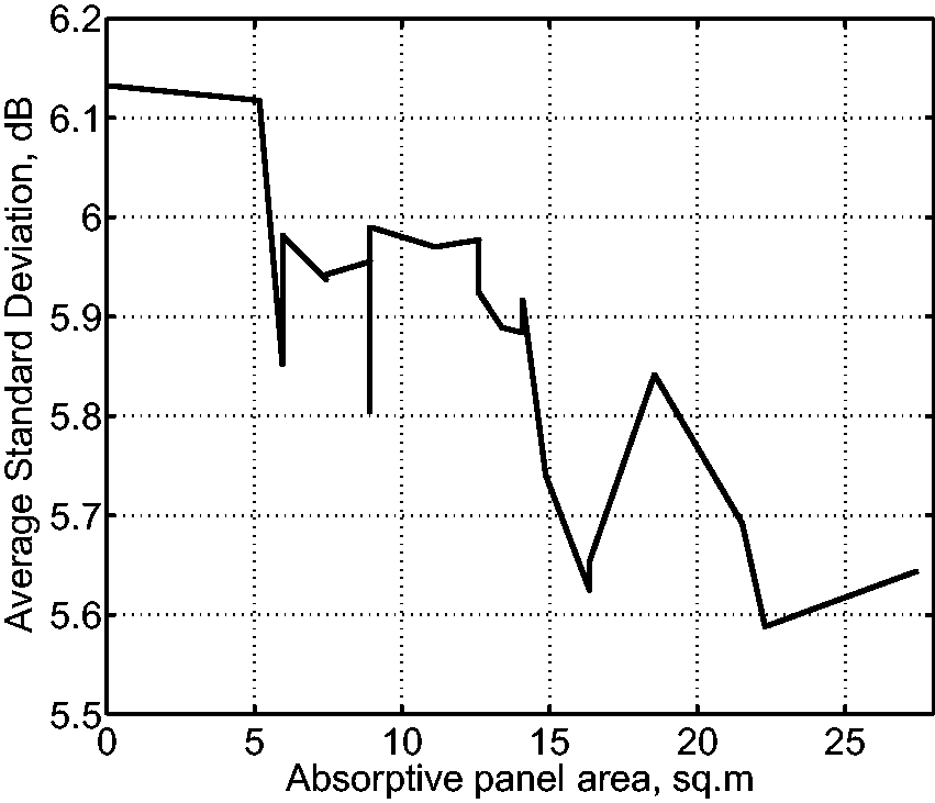
Average standard deviation against the absorption area.

A significant $\bar{S D}$ decrease can be observed when the room configuration from “Only corner absorption” (5.17 m²) changes to “Inner ceiling absorption” (5.95 m²), while $\bar{S D}$ increase may also be noted in the configuration “Wall absorption with corner” (5.84 m²) when compared to the “Outside absorption with center side walls and ceiling” configuration (5.65 m²). This may be caused by the low sound absorption of the absorbing materials at low frequencies. Bass traps commonly used in the industry include a reactive absorption mechanism which should improve the performance.

Another point of interest in the analysis of Figure 5 is the comparison between model iterations containing the same amount of absorption but located in different positions in the room. Three room absorption configurations contained 8.92 m² of absorption area but returned three different average standard deviation values ranging from 5.99 dB to 5.80 dB. The three configurations returned different average standard deviation values while utilizing the same absorption area which suggests that location of the absorption does have an effect on the performance of the space. The absorption location dependence will be further analysed and discussed in a section to follow and will help further the definition of the most optimum room treatment for the frequency response and the sound field.

Comparison of the standard deviation sound field

Another objective of this study was to investigate the effect of the added absorption on the entire listening area. The grid plane described previously highlights this concern.

Analysis of sound field changes due to absorption addition

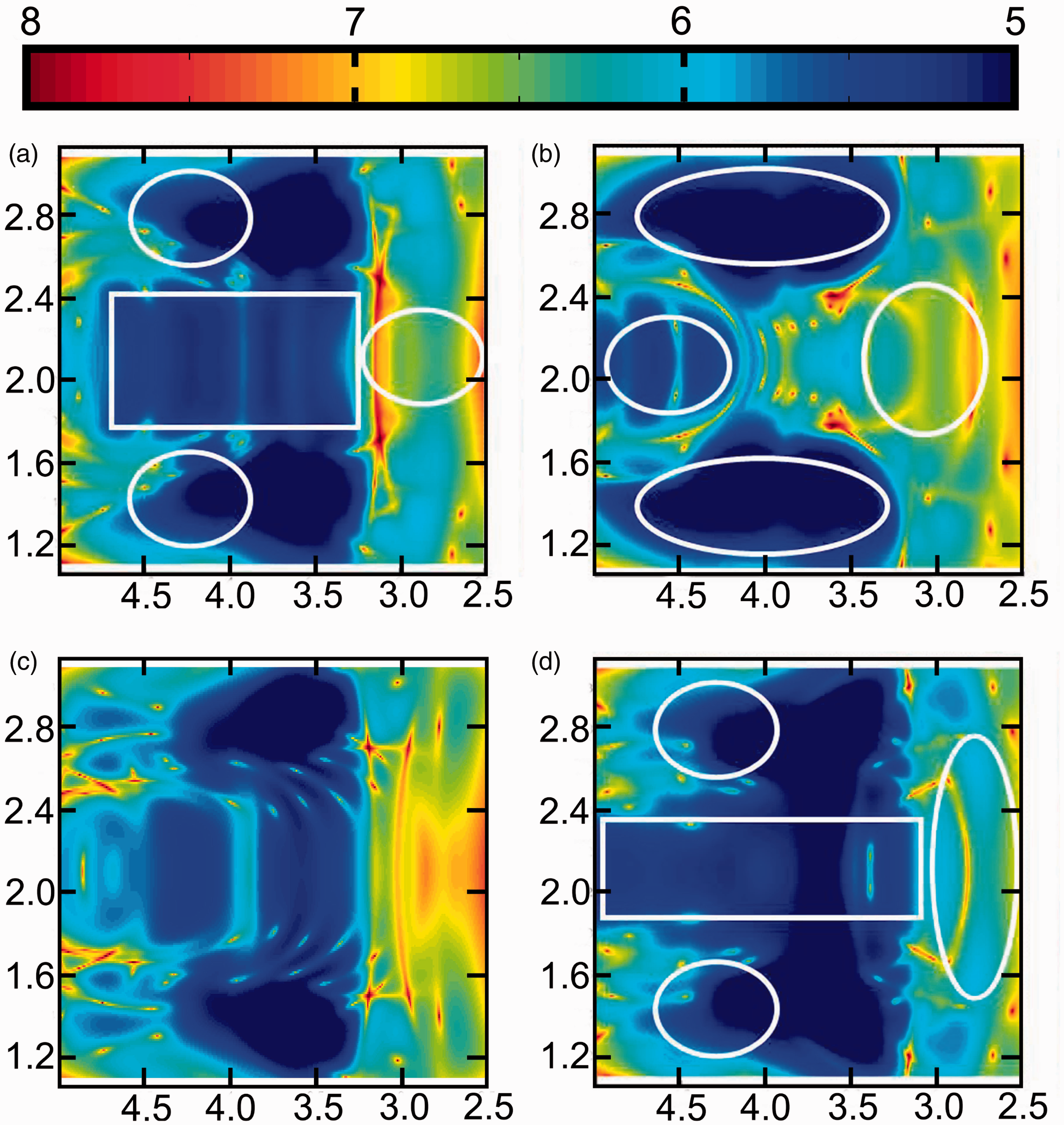
Figure 6 displays the standard deviation of each grid point in the listening region for four of the absorption configurations analysed. Blue areas in the figures represent areas of low standard deviation and acceptable listening positions, while red areas represent locations of higher standard deviation and correlate to areas with poor listening positions. The results in these figures show that the absorption treatment configurations do have an effect on the standard deviation. The standard deviation values for each individual listening position within the listening region ranged from approximately 4.5 dB up to almost 10 dB.

Figure 6.

Standard deviation sound fields: The blue areas of the figures represent areas of low standard deviation and acceptable listening positions, while the red areas represent locations of higher standard deviation (Unit: dB).(a) No absorption. (b) All absorption. (c) Only corner absorption. (d) All absorption no corners.

Figure 6(a) shows the sound field for a room without any absorption, and mode shapes (i.e. standing waves) clearly dominate the low-frequency performance of the listening positions. The linear and geometrical shape of areas with higher standard deviation indicates modal resonance at that location dominating the standard deviation of the frequency response, while some positions in close proximity of such locations may be acceptable. Strong modal effects are evidenced in these regions. In contrast, Figure 6(b) displays the sound field for the room with all 34 absorptive panels active. This room configuration shows how dramatically the location of acceptable listening positions changes. Whereas in Figure 6(a) the acceptable listening positions were in small isolated regions of the listening area, in Figure 6(b), with the addition of absorption, there were more widespread areas with acceptable listening positions. This change was especially evident between 3.5 and 4.5 m along the length and at approximately 0.5 m on either side of the room’s centre line. There was also another notable region of acceptable listening positions in the rear of the listening region near 5 m along length and centered along the width. Similar comparisons can be made between the rooms with no absorption (Figure 6(a)), with only corner absorption active (Figure 6(c)), and all absorption excluding corners (Figure 6(d)). These figures indicate that the addition of the absorption to the room for modal damping had an impact on the location and quality of the low frequency listening positions within the space.

Analysis of sound field changes due to absorption location

An interesting observation arising from Table 3 relates to the difference in the average standard deviation for various configurations with the same active total absorption area in the space. As discussed previously; there were three configurations with 8.92 m² of total absorption area. Upon further investigation, it can be seen that the three absorption configurations with 8.92 m² of active absorption were (1) outside absorption with outside ceiling, (2) ceiling absorption equivalent on walls, and (3) only ceiling absorption. The range of average standard deviation values for these three configurations spanned from 5.99 dB to 5.80 dB. The fact that the configuration with only the ceiling panels active had the lowest average standard deviation by a significant margin led the authors to investigate the effects of the ceiling on the performance of the space by performing iterations with and without ceiling absorption active.

Table 4 conveys the average standard deviation of seven absorption configurations coupled with the respective absorption configuration with the absorptive ceiling panels active. The results for the addition of the ceiling absorption show a clear pattern of improving the sound field. Each of the seven comparisons significantly improves the average standard deviation of the sound field by at least 0.20 dB with an average of 0.27 dB. The ceiling absorption showed a clear improvement in every comparison, while a similar study for other absorption locations (results not shown) did not show such dramatic improvements due to porous absorptions ineffectiveness compared to pressure-based absorption at high acoustic pressure locations.

Table 4.

Ceiling absorption investigation.

Absorption configuration	TotalAbsorptionArea (m²)	$\bar{S D}$ (dB)	Difference due to added Absorption
No absorption	0.00	6.13
Only ceiling absorption	8.92	5.80	0.33
Only corner absorption	5.17	6.12
Ceiling absorption with corners	14.09	5.88	0.23
Outside wall absorption	5.95	5.98
Outside absorption with ceiling	14.86	5.74	0.24
Only side wall absorption	7.43	5.94
Side wall absorption with ceiling	16.35	5.62	0.31
Outside wall absorption with center side wall	7.43	5.94
Outside absorption with center side wall and ceiling	16.35	5.65	0.29
Side wall absorption with corners	12.60	5.98
Side wall absorption with corners and ceiling	21.52	5.69	0.29
Wall absorption with corners	18.55	5.84
All absorption	27.47	5.64	0.20

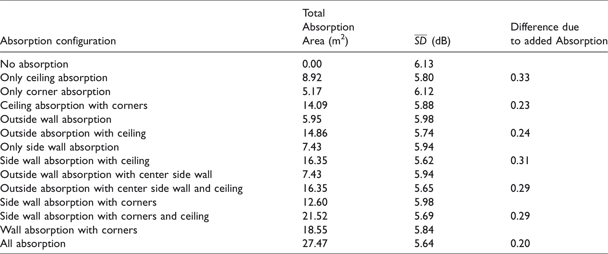
Figure 7(a), (b) and (d) conveys the results for three absorption configurations and their coupled configurations with the ceiling absorption added. As was shown in Table 4, the ceiling absorption had a much more prominent effect on the average standard deviation of the listening region than did the corner absorption. This effect on the sound field can be clearly seen in the figures.

Figure 7.

Standard deviation sound fields for the effects of ceiling absorption: The blue areas of the figures represent areas of low standard deviation and acceptable listening positions, while the red areas represent locations of higher standard deviation (Unit: dB). (a) Only ceiling absorption. (b) Ceiling absorption with corners. (c) Only side wall absorption. (d) Side wall absorption with ceiling.

The three base configurations analysed for the addition of ceiling absorption were no absorption, only corner absorption, and only side wall absorption in Figures 6(a) and (c), and 7(c), respectively. Each comparison showed a dramatic reduction in overall standard deviation and each reveals similar improvement characteristics to the sound field. Figure 6(a), which displays the sound field for the room without any absorption, had many areas with high standard deviation and showed the highest overall standard deviation of any room configuration. Adding the 8.92 m² of absorption to the ceiling yielded a much smoother response as can be seen in Figure 7(a). Many of the high standard deviation areas were removed through the centre of the room along the length of the listening region.

An improvement was also seen between 3 m and 4.5 m along the length of the listening region and 0.5 m on either side of the centre of the listening region. These areas of improvement were marked with white circles and white rectangles on the figures containing the ceiling absorption. Figure 7(a), with just the ceiling absorption active, had the smoothest low-frequency sound field and lowest average standard deviation of any configuration with equal or lesser amounts of absorption. In fact, it was not until the absorption in the room was nearly doubled that there was another configuration that bettered that of Figure 7(a).

Similar improvements were also seen between Figures 6(c) and 7(b) as well as between Figure 7(c) and (d). Here, the white circles and rectangles also represent the areas in which the sound field was improved by adding the ceiling absorption. Most areas of the listening region were improved after the addition of ceiling absorption; however, the most extensive improvements were noted along the centre of the width of the room between 3 m and 4.5 m in the x direction and also along the sides of the listening region. Also, the ceiling absorption was effective at reducing the higher standard deviation areas near the front of the listening region, in the areas less than 3.5 m in the x direction. Corner absorption was of little help in these areas, and in some cases, even degraded them.

Conclusions

An approach has been proposed and developed to qualify the sound field and the frequency response due to the addition of absorption in a room. Frequency responses at various listening positions were evaluated by the standard deviation at the chosen frequency range across the listening region. The addition of absorption to the room had a clear effect on the average standard deviation of the listening region. With the addition of the absorption to the room, the average standard deviation of the listening room was reduced and the average acceptable listening positions were improved on a whole. This claim was also supported by the 2D sound field plots over the listening areas which showed improvements after the addition of absorption to the room. However, the trend observed, that the addition of damping by absorption improves low-frequency response quality, is rather loose as some absorption locations are more effective at improving the low-frequency sound field than others.

There were several instances to suggest that absorption configurations with the same active absorption area can affect the sound field differently suggesting location dependence of the performance. The large difference in the depiction of the standard deviation sound field plots also suggests that the location of the absorption had a significant effect on shaping the listening region. The standard deviation sound field plots showed widened areas of acceptable listening positions for rooms with some sort of absorption added, but also showed that some absorption locations greatly affect the sound field in predictable locations, while other absorption locations have little to no effect on the sound field.

Footnotes

Declaration of conflicting interests

The author(s) declared no potential conflicts of interest with respect to the research, authorship, and/or publication of this article.

Funding

The author(s) disclosed receipt of the following financial support for the research, authorship, and/or publication of this article: This work was supported by a grant (S.K. Lau) from the University of Nebraska-Lincoln.

References

Bolt

RH.

Note on the normal frequency statistics in rectangular rooms. Appl Acoust 1946; 18: 130–133.

Morse

PM.

Vibration and sound. 2nd ed. New York: Acoustical Society of America, 1948.

Iannace

Acoustic correction of monumental churches with ceramic material: the case of the Cathedral of Benevento (Italy). J Low Frequen Noise Vib Active Control 2016; 35: 230–239.

Sahu

Tuhkuri

Active structural acoustic control of transmitted sound through a double panel partition by weighted sum of spatial gradients. J Low Frequen Noise Vib Active Control 2017; 36: 27–42.

Bagha

Modak

SV.

Active structural-acoustic control of interior noise in a vibro-acoustic cavity incorporating system identification. J Low Frequen Noise Vib Active Control 2017; 36: 261–276.

Lau

Tang

SK.

Spatial attenuation of sound in a rectangular enclosure under active control of sound transmission through an elastically supported flexible panel. J Low Frequen Noise Vib Active Control 2008; 27: 147–165.

Cui

Chen

Modelling and analysis of acoustic field in a rectangular enclosure bounded by elastic plates under the excitation of different point force. J Low Frequen Noise Vib Active Control 2017; 36: 43–55.

Kleiner

Tichy

Acoustics of small rooms. ▪: CRC Press.

Howard

Angus

Acoustics and psychoacoustics. 2nd ed. Oxford, UK: Focal Press, 1998

10.

Angus

JAS.

The effect of diffusers on frequency-dependent room mode decay. J Audio Eng Soci1999; 47.

11.

Louden

Dimension ratios of rectangular rooms with good distribution of eigentones. Acoustica 1971; 24: 101–104.

12.

Bonello

OJ.

A new criterion for the distribution of normal room modes. J Audio Eng Soc 1981; 29: 597–606.

13.

Walker

Low frequency room responses, part 2 – calculation methods and experimental results. BBC Res Devlop 1992; 93.

14.

Cox

D’antonio

Avis

Room sizing and optimization at low frequencies. J Audio Eng Soc 2004; 52: 640–650.

15.

Bolt

RH.

Normal modes of vibration in room acoustics: angular distribution theory. J Acoust Soc Am 1939; 11: 74–79.

16.

Mehta

Johnson

and

Rocafort

Architectural acoustics: principles of design. 1st ed. Upper Saddle River: Prentice Hall, 1998.

17.

Morse

Ingard

KU.

Theoretical acoustics. New Jersey: Princeton University Press, 1986.

18.

Olive

Schuck

Ryan

JG.

The detection thresholds of resonances at low frequencies. J Audio Eng Soc 1997; 45: 116–127.

19.

Schuck

Olive

Ryan

et al . Perception of perceived sound in rooms: some results of the Athena project. In: Proceedings of the AES 12th international conference: perception of reproduced sound, Copenhagen, Denmark, June 28–30, pp.49–73. Copenhagen, Denmark: Audio Engineering Society.

20.

Toole

FE.

The measurement and calibration of sound reproducing systems. J Audio Eng Soc 2015; 63: 512–541.

21.

Karjalainen

Antsalo

Mäkivirta

et al . Perception of temporal decay of low-frequency room modes. In: AES 116th convention, Berlin, Germany, 8 May–11 May 2004.

22.

Toole

FE.

Loudspeakers and rooms for sound reproduction – a scientific review. J Audio Eng Soc 2006; 54: 451–475.

23.

Avis

Fazenda

Davies

Thresholds of detection for changes to the Q factor of low-frequency modes in listening environments. J Audio Eng Soc 2007; 55: 611–622.

24.

Fazenda

Avis

Davies

WJ.

Perception of modal distribution metrics in critical listening spaces – dependence on room aspect ratios. J Audio Eng Soc 2005; 53: 1128–1141.

25.

Fazenda

Wankling

Hargreaves

Subjective preference of modal control methods in listening rooms. J Audio Eng Soc 2012; 60: 338–348.

26.

Fazenda

Stephenson

Goldberg

Perceptual thresholds for the effects of room modes as a function of modal decay. J Acoust Soc Am 2015; 137: 1088–1098.

27.

Van Nieuwland

Weber

Eigenmodes in nonrectangular reverberation rooms. Noise Control Eng 1979; 13: 112–121.

28.

Papadopoulos

Redistribution of the low frequency acoustic modes of a room: a finite element-based optimization method. Appl Acoust 2001; 62: 1267–1285.

29.

Everest

Pohlman

Master handbook of acoustics. New York: McGraw Hill, 2009.

30.

Eda

Yosuke

, and Tetsuya

Acoustical effects of columns, beams and furniture on sound field in small enclosures. Int Cong Acoust 2010; pp. 23-27.

31.

Welti

TS.

Subwoofer optimization in rooms for consistency and efficiency. J Acoust Soc Am 2011; 130: 2334

32.

Allard

Atalla

Propagation of sound in porous media: modelling sound absorbing materials. 2nd ed. West Sussex, UK: John Wiley & Son, 2009.

33.

Delaney

Bazley

EN.

Acoustical characteristics of fibrous absorbent materials. Appl Acoust 1969; 3: 105–116.

34.

Bies

Hansen

CH.

Flow resistance information for acoustic design. J Audio Eng Soc 1979; 13: 357–391.

Effects of absorption placement on sound field of a rectangular room: A statistical approach

Abstract

Keywords

Introduction

Numerical modelling

Room model

Boundary conditions and mesh size

Sound source and model verification

Sound absorption modelling

Analysis methods

Results and discussions

Comparison of the average standard deviation

Comparison of the standard deviation sound field

Analysis of sound field changes due to absorption addition

Analysis of sound field changes due to absorption location

Conclusions

Footnotes

Declaration of conflicting interests

Funding

References