
Abstract
Structural control of a multi-degree-of-freedom building under earthquake excitation is investigated in this paper. The ARMAX model calculation is developed for a linear representation of multi-degree-of-freedom structure. A control approach based on the generalized minimum variance algorithm is developed and presented. This approach is an empirical method to control the story unit regardless of the coupling with other stories. Kanai-Tajimi and Clough–Penzien models are used to generate the seismic excitations. Those models are calculated using the specific soil parameters. In order to test the control strategy performances under real strong earthquakes, the structure has been subjected to EL Cento earthquake. RST controller form shows the stability conditions and the optimality of the control strategy. Simulation tests using a 3DOF structure are performed and show the effectiveness of the control method using of the empirical method.
Keywords
Introduction
The impact of control theory in the different domains of engineering and applied sciences has become increasingly important in the last few decades.1,2 Researchers are very interested in control against the external disturbances (vehicles, buildings, sensors disturbances, etc.).2–8 One of the important missions of structural control is to ensure the safety of structures and cities during large earthquakes.9–13 In fact, Weng et al. 14 have proposed the finite-time vibration control of earthquake-excited linear structures with input time-delay by considering the saturation. The objective of designing controllers is to guarantee the finite-time stability of closed-loop systems while attenuating earthquake-induced vibration of the structures. Gudarzi 15 has presented a robust μ-synthesis output-feedback controller design for seismic alleviation of multi-structural buildings with parametric uncertainties and to tackle the instabilities and performance declines due to these uncertainties. Tınkır et al. 16 have investigated a SolidWorks and SimMechanics-based dynamic modeling technique and displacement control of flexible structure system against the disturbance through theoretical simulation and experimental approach. PI and LQR controllers have been used as a control strategy in the active mode. Both simulation and experimental results have shown the reduction of vibration due to the disturbance effects.
A multi-degree-of-freedom (MDOF) structure can be considered as a large-scale system with interconnected subsystems, which are story units. The problem of interconnection between the story units and the structural properties of the building is considered as a whole and must be addressed. The interconnection effects can also be introduced in the control law formulation, or can be considered as external disturbances to be compensated by control actions. Another problem encountered in MDOF structural control is the number and location of actuators. Several structural models have been studied and developed for control perspective: state space, ARMAX (autoregressive moving average exogenous), etc. Alqado et al.17 developed five methods for structural identification approach, specifically ARX, ARMAX, BJ, OE, and state-space models, and have implemented them for the identification process. Furthermore, the paper shows that the ARMAX and the output error models had indicated an excellent performance to predict the mathematical models of vibration's propagation in the building. The ARMAX model can give an interesting representation of the system for a digital control perspective. In this case, the system is characterized as stochastic process described by a linear model subjected to external disturbances. Ying et al. 17 proposed an algorithm for the decentralized structural control of tall shear-type buildings under unknown earthquake excitation. A decentralized control algorithm based on the instantaneous optimal control scheme was developed with limited measurements of structural absolute acceleration responses. The inter-connection effect between adjacent substructures was treated as ‘additional unknown disturbances’ at substructural interfaces to each substructure. However, the control algorithm is based on the minimization of some cost functions such as linear quadratic regulator (LQR) which requires a solution of the Riccati equation. This one is subjected to a boundary condition at the terminal time that leads to a sub-optimal solution. So, in such perturbed systems, the controller performances and robustness may be weak. 18
The purpose of this paper is to develop a control strategy applied to an earthquake excited 3DOF structure. This algorithm attempts to minimize a generalized cost function including variance of both output and control effort. For this purpose, a specific model of the system to be controlled and its environment will be developed.
The GMV algorithm has been widely studied in literature. It was introduced by Clarke19,20 as an extended version of the minimum variance (MV) algorithm initially developed by Åström.21–23 Our approach presented in this paper is a generalization of the GMV algorithm for the multivariable case. A multivariable ARMAX model of the structure is used.
Our approach is a method that uses the mono-variable GMV controller for each story. The coupling terms appearing in the structural model are not introduced in control law formulation but rather they are considered as external perturbations to be compensated by the control actions. The ARMAX polynomial parameters are not tuned; they are calculated according to the structural parameters. Also, the soil characteristics described by the dynamical model (Kanai-Tajimi, Clough-Penzien) can be introduced within the structural model that leads to an optimal prediction and also defines the stability conditions that take the soil parameters into account. In other words, the poles of the polynomial C(q−1) are the closed-loop poles which are related to the introduction of the soil parameters.
The paper is organized as follows: the next section deals with the development of the dynamic model of the structure, while the following section deals with the presentation of the MIMO ARMAX model. The GMV algorithm is introduced in the subsequent section. The seismic excitation models are then presented.. Then, in the next section, simulation results showed the effectiveness of the developed algorithms. Finally, some conclusions are given.
Dynamical model of an MDOF structure
The purpose of this section is to develop the dynamical model of an MDOF structure under seismic excitation. Figure 1(a) is a schematic representation of the structure. It is a multi-story building with active tendon controllers in each story unit. In order to establish the dynamical model, the following assumptions are considered
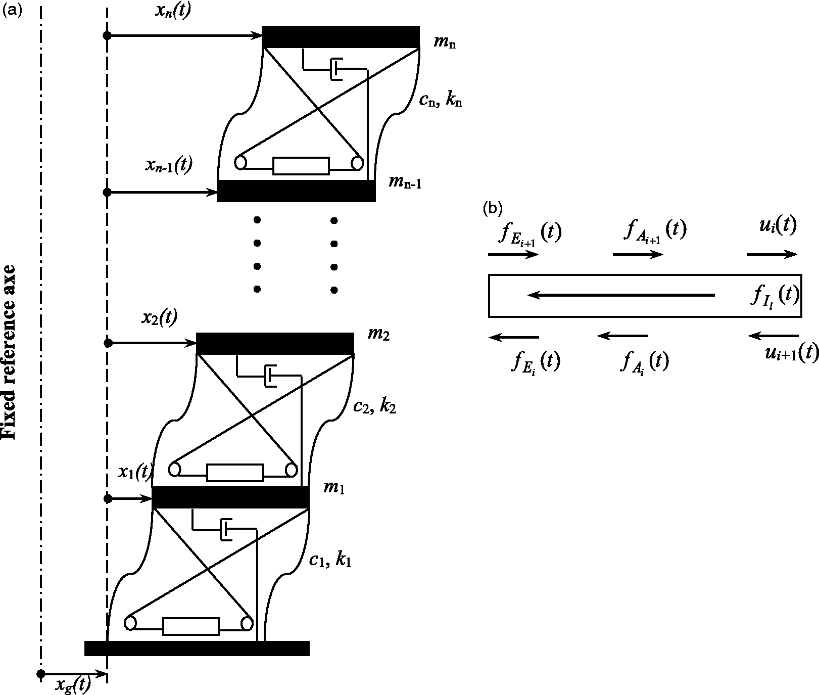
Schematic representation of a multi-degree-of-freedom structure under seismic excitation (a) motion of the structure (b) forces equilibrium of the ith story unit.
(1) Each story is supposed to be a lumped mass in the girder.
(2) The two vertical axes between two adjacent floors are weightless and inextensible in the vertical direction.
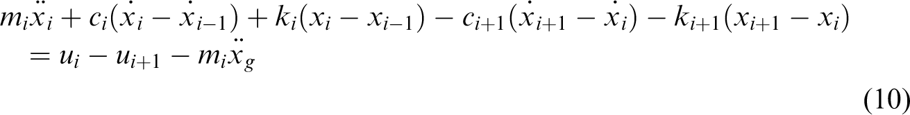
Figure 1(b) is a representation of the dynamic force equilibration at the ith story unit, which can be written as
24


Absolute displacement

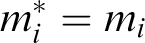
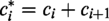
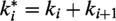
The ith story unit is characterized by its characteristic parameters. In this system, it is assumed that the structural mass, mi, and the elastic stiffness, ki, have been concentrated in floors and columns, respectively. Internal viscous damping, ci, is also a parameter that describes the structural behavior.
Substituting equations (2) to (5) into equation (1), we obtain
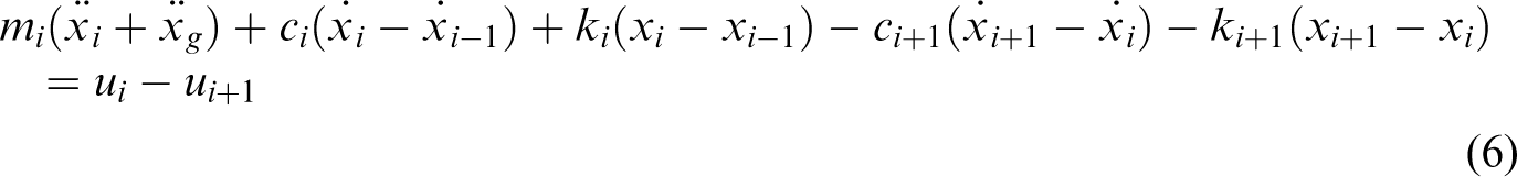
Equation (6) can be written in the matrix form as
24

M is the (n × n) mass matrix of the structure.
C is the (n × n) damping matrix of the structure.
K is the (n × n) stiffness matrix of the structure.
L is the (n × 1) matrix indicating the location of actuators.
Iv =[1 1……1] T unity vector of dimension (n × 1).
ARMAX model of the structure
We are interested in this section to derive the ARMAX model of the MDOF structure.
Structural model
Consider the state space equation of the MDOF structure which can be obtained from equation (7) by choosing
I is the identity matrix of dimension (n × n)
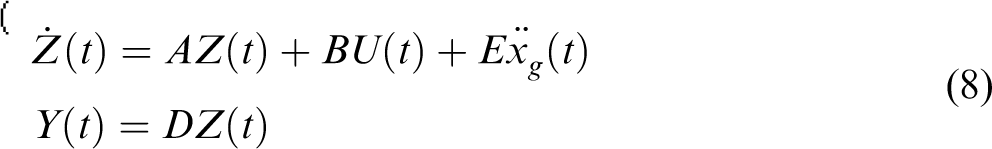
The digital control of the system needs the knowledge of the discrete representation model. Thus, the discrete model, described by equation (8), can be written in the following form24–26

q−1 shift operator is defined as
Empirical model
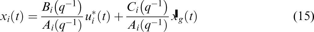
Our calculation for the empirical model is based on a re-parameterization of the structural model. This is done to obtain a decoupled model where the interactions between stories are considered to be external perturbations. Considering the dynamical equation of motion of the ith story
Equation (10) can be written as
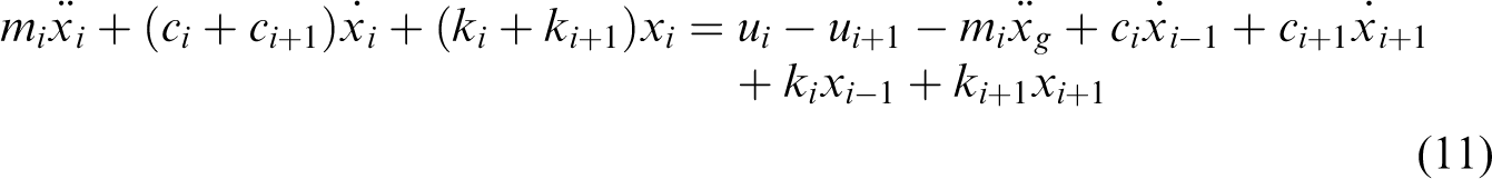
Introducing new notations, equation (11) has the form

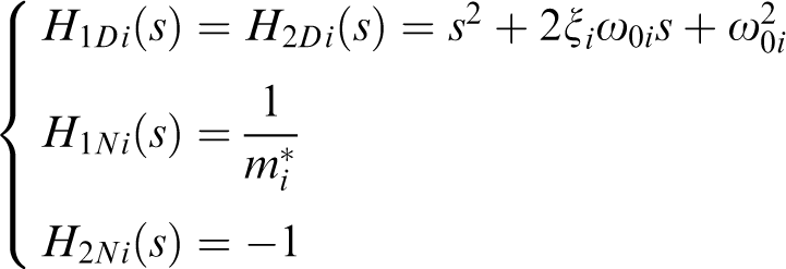
Equation (12) can be interpreted as a new decoupled subsystem with new structural parameters, new control variable and a term of perturbations. The ARMAX model of each subsystem is determined from equation (12). By neglecting the term

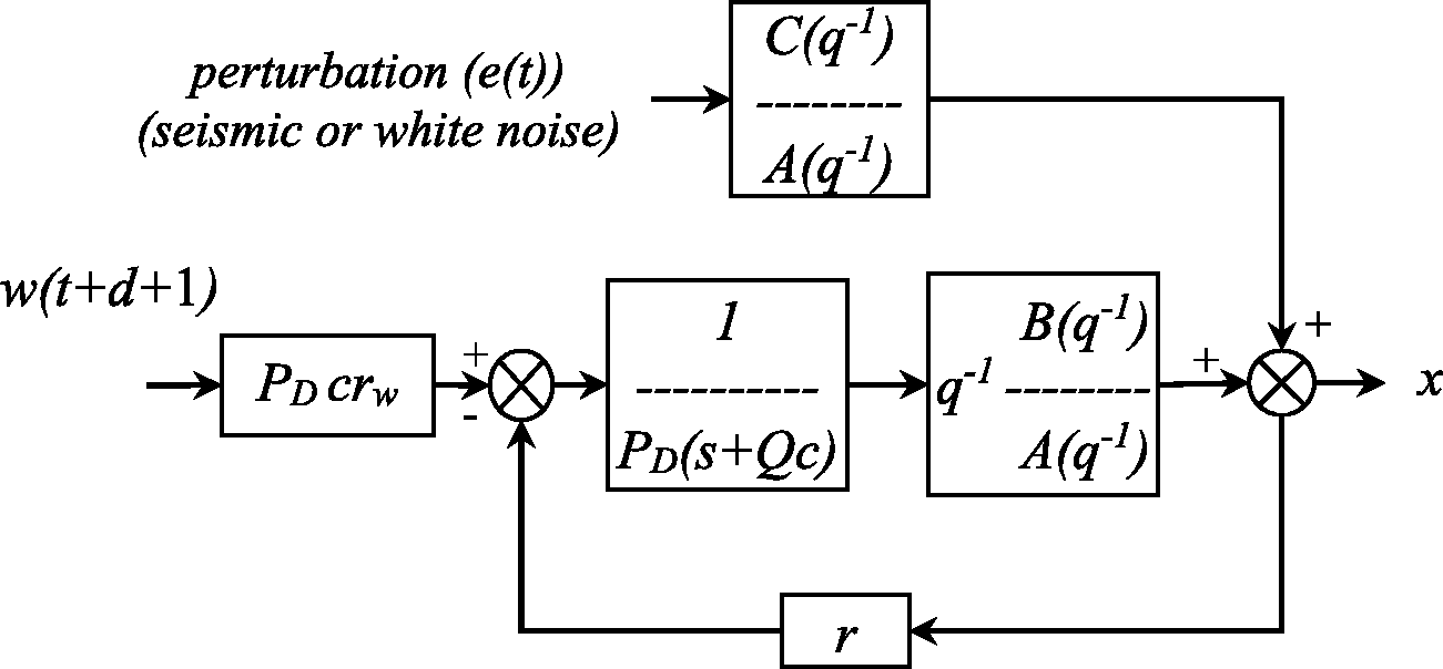
Figure 2 shows a bloc diagram of the ith story model.
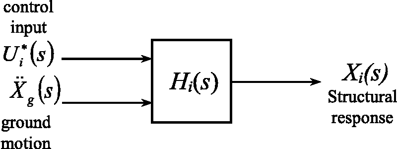
Bloc diagram of the ith story model.
Depending on the model of seismic excitation, we develop different ARMAX models that can be obtained, and the following cases arise.
Case 1
The seismic excitation model is unknown or is not taken into consideration. Equation (13) has the form

The ARMAX model of the structure is obtained by the discretization of equation (14)
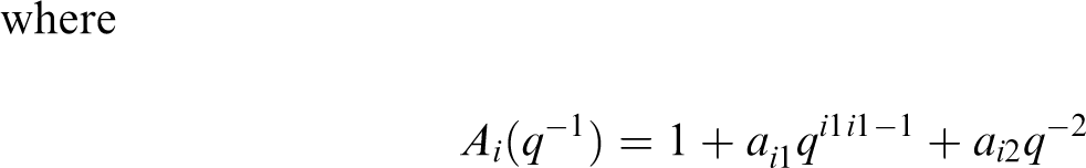
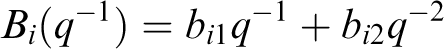
By analytical discretization of equation (14) using the Z-transform, the polynomial parameters are given by
5
Case 2
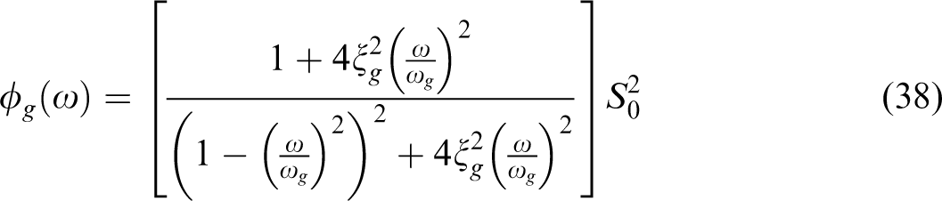
The ground acceleration is described by the Kanai-Tajimi model, i.e.

E(s) is the Laplace transform of white noise.
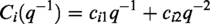
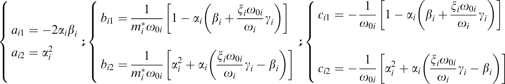
Substituting equation (16) into equation (13), we obtain
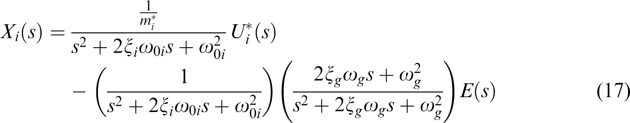

By reducing the second member of equation (18) to a common denominator, we obtain

Block diagrams are shown in Figure 3 to illustrate the previous calculations.
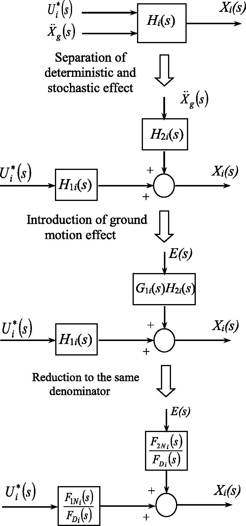
Block diagram of ith story model under Kanai-Tajimi seismic excitation.
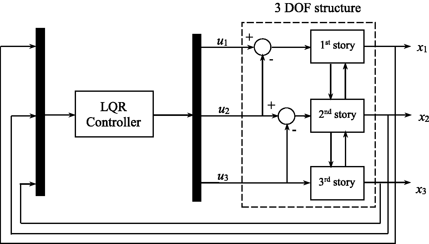
Schematic representation of the LQR approach for a 3DOF structure. LQR: linear quadratic regulator.
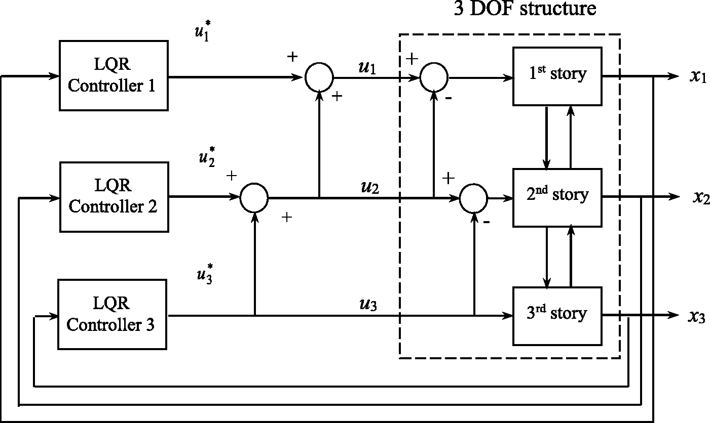
Schematic representation of the empirical LQR approach for a 3DOF structure. LQR: linear quadratic regulator.

Schematic representation of the GMV approach for a 3DOF structure. GMV: generalized minimum variance.
Discretization of equation (19) gives the discrete ARMAX model of the structure under the Kanai-Tajimi ground acceleration 18
LQR algorithm
Control algorithms for linear systems have been extensively studied. Optimal control algorithms are based on the minimization of a quadratic performance index whose objective is to maintain the desired system state while minimizing the control effort. 1
LQR for MDOF structure
The LQR is applied for the system represented in equation (8). In this case, the control gain matrix is determined as
1
P is the solution of Riccati equation given as

LQR using the empirical model
In this case, we develop an LQR controller which is calculated for each story of the structure. The controller is designed based on the structural model represented by equation (12). Each controller is calculated using an SDOF structural model of the ith storey by ignoring the coupling terms, represented by the term, due to the interconnection with other subsystems.

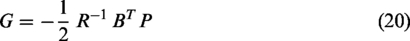
Using the state space concept, equation (22) can be written as

In this case, the control gain matrix is

Pi is the solution of Riccati equation given as

Generalized minimum variance control algorithm
The generalized minimum variance (GMV) algorithm was introduced by Clarke20,21 to control the non-minimum phase systems. It is an extension of the MV algorithm 26 which, by choosing a certain performance criterion and a certain model of the controlled system and its perturbations, attempts to minimize the variance of the output.
GMV control algorithm for MDOF structure
A generalization of the GMV algorithm for multi-input-multi-output (MIMO) systems has been proposed for structures under earthquakes. The controlled system in this case is assumed to be described by a linear vector difference equation including a moving average of white noise.
The criterion to be minimized is

E is the expected value w(t + d + 1) is the n × 1 vector defining the reference signal.
P, Rw,
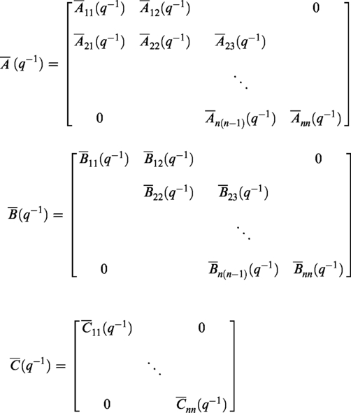
In the MIMO case, we proceed by discretization of the state space model described by equation (8), we obtain full matrix model.
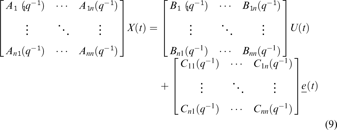
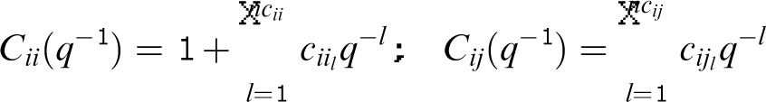
The discrete multivariable ARMAX model is then obtained. It is given by

As in the mono-variable case, we first have to derive the optimal predictor

Using equations (27) and (28), it is shown that the control strategy is given by

We have shown the efficiency of this control strategy, but the major problem of this method is the huge calculation matrix of Diophantine equation. There is a problem of implementation, control calculation and also problem of the coupling terms that are taken into consideration.
Empirical GMV control algorithm for the structure
The aim of this work is the calculation of one model (the empirical model) that permits us the generalization of the SISO GMV algorithm to the MIMO case without any further modification. So, we calculate the decoupled model by ignoring the interaction term (ϕi*). So we can obtain a mono-variable linear time varying system for each story for the structure.
To derive the GMV algorithm, the ARMAX model of the system is used
7


The performance index to be minimized is

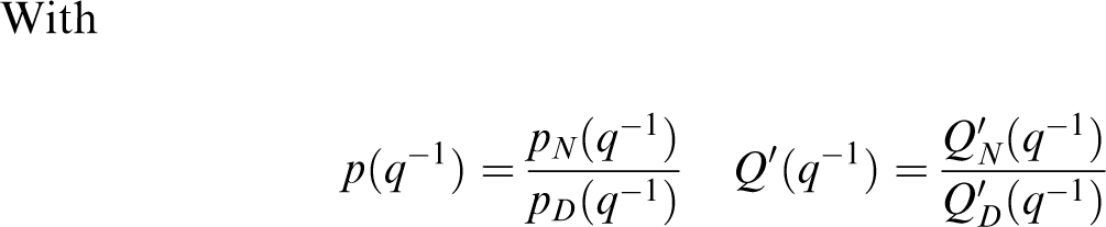
The degrees of P and rw can be chosen arbitrarily. We remark in this criterion that w(t + d + 1) is a disposable information, but y(t + d + 1) is not. It is the future information that we must predict. After some calculations, the prediction of py(t + d + 1) = ψ(t + d + 1) is (see Appendix 1)


With


The minimization of J leads to the GMV control law given by (see Appendix 2)
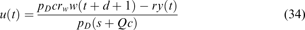
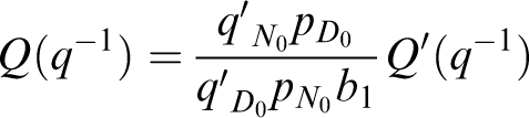
The controller described by equation (34) is written on the RST form2,21

The closed loop transfer function is deduced from equation (35)

The resulting closed-loop poles associated to an RST controller are the poles of the polynomial C(q−1) (with: PN =1) according to the Diophantine equation described by equation (33). We can remark that similar tracking behavior with the pole placement can be obtained. The polynomial C(q−1) defines the tracking trajectory regulation, and the closed-loop dynamic at the same time
18

So the polynomial parameters C(q−1) lead to an optimal prediction. Moreover, the closed loop characteristic polynomial is C(q−1) = T(q−1), and it also defines the closed loop stability condition, where the poles must be in the unit circles.
19
The empirical model derived previously is used to implement the monovariable case of the GMV to each story independently. Figure 8 is a schematic representation of this control approach. Our contribution is to calculate the GMV controller that has the charge to compensate the perturbations, represented by the term
Generalized minimum variance control architecture.
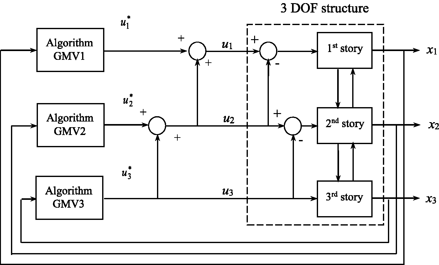
Schematic representation of the empirical GMV approach for a 3DOF structure. GMV: generalized minimum variance.
Mathematical model of earthquake ground motion
The earthquake ground acceleration is modeled as a uniformly modulated non-stationary random process.
23

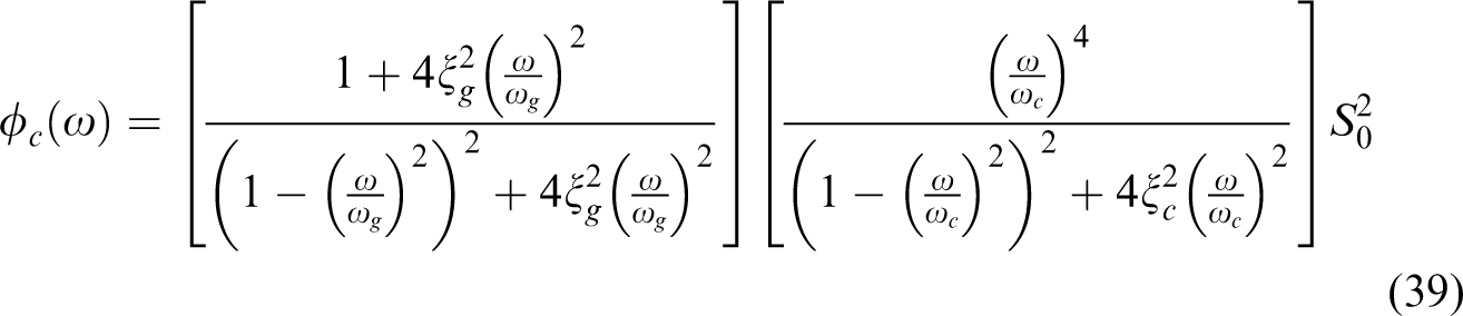
Using such a second high-pass filter, the Kanai-Tajimi spectrum is modified as follows to obtain the Clough–Penzien spectrum
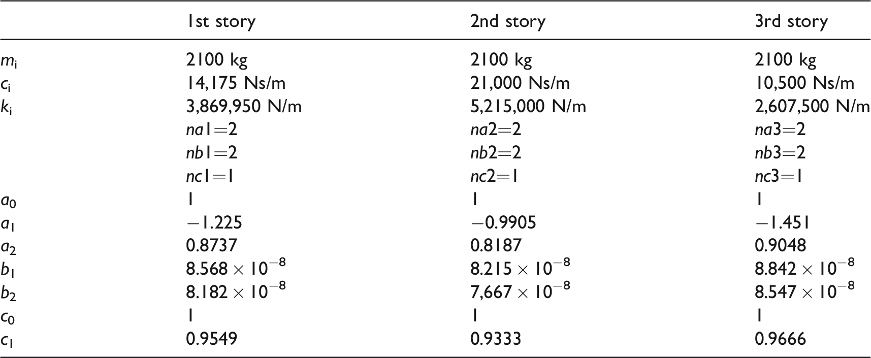
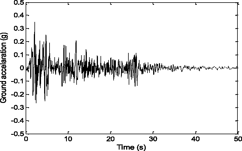
A particular envelope function ψ(t) given in the following will be used
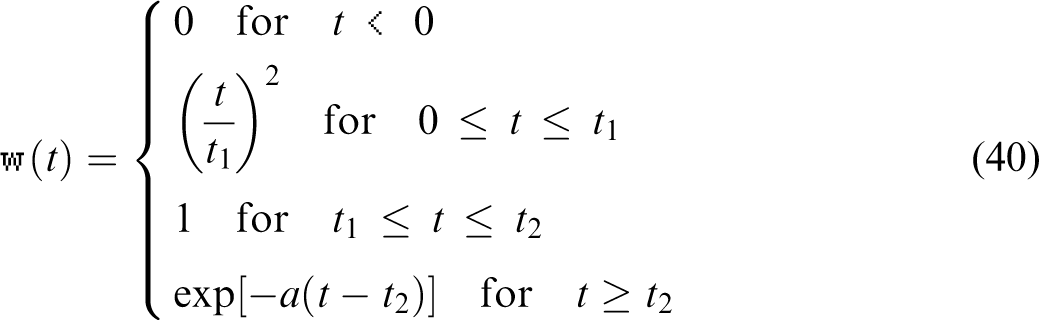
The Kanai-Tajimi and Clough–Penzien ground accelerations have been simulated and are presented in Figure 9.
Simulated ground accelerations.
Simulation results
Simulation tests are performed using a 3DOF structure with the following structural parameters 11
m1=2100 Kg, k1=1,262,450 N/m, c1=3675 Ns/m
m2=2100 Kg, k2 = 2,607,500 N/m, c2=10500 Ns/m
m3=2100 Kg, k3=2,607,500 N/m, c3=10500 Ns/m
An active tendon controller is installed in every story unit and the angle of incline of the tendons with respect to the floor is 25°. Thus, the control force vector from the controllers is u/cos25°. Thus, we can suppose that the force is applied at the top of each story and assumed to be activated externally by an independent power supply.
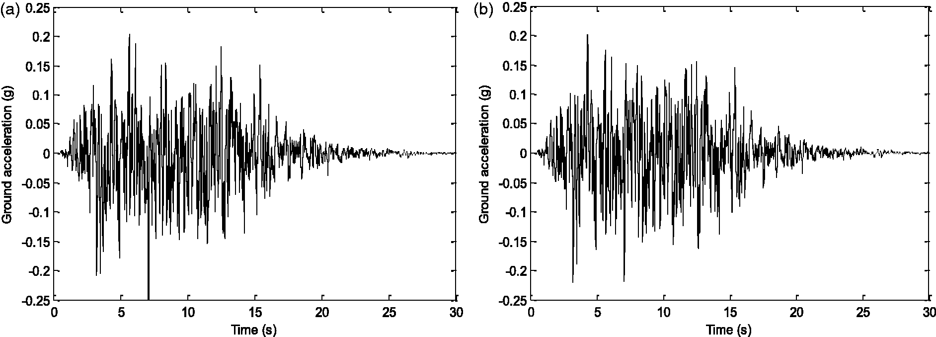
To implement the empirical approach, Table 1 gives the structural parameters, and the corresponding ARMAX model for each story.
Structural parameters and ARMAX model parameters.
ARMAX: autoregressive moving average exogenous
Ponderation polynomials used in the GMV algorithm are

In order to test the control strategy performances under real strong earthquakes, the structure has been subjected to EL Cento earthquake as presented in Figure 10. The Empirical GMV control algorithm has demonstrated good performances.
El Centro Earthquake.
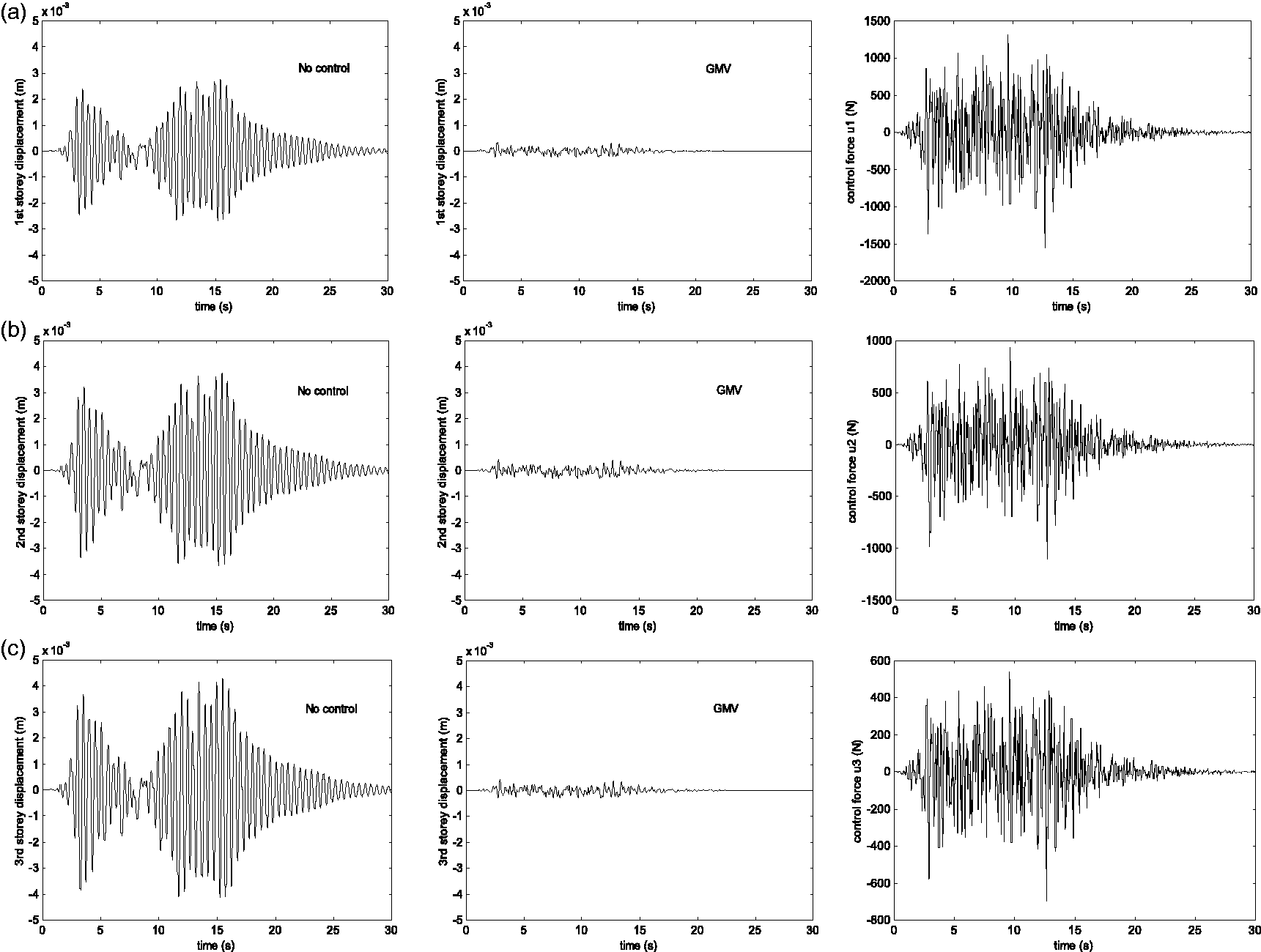
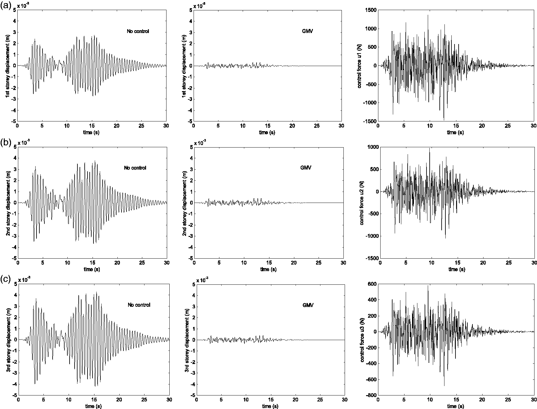
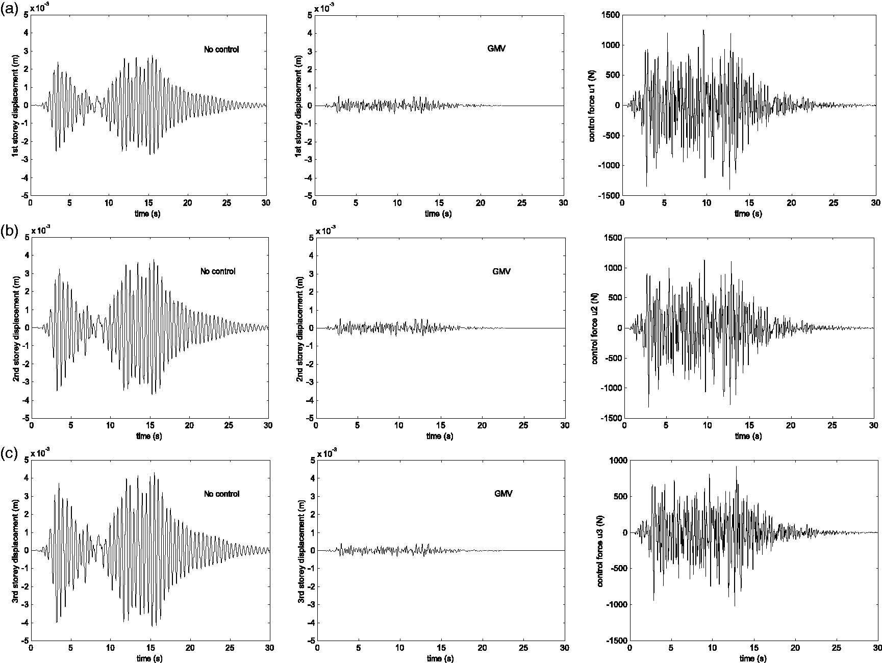
Responses of the structure to Kanai-Tajimi and Clough–Penzien excitation models are shown in Figures 11 to 22.
In order to demonstrate the effectiveness of our approach, several simulation comparisons have been made.
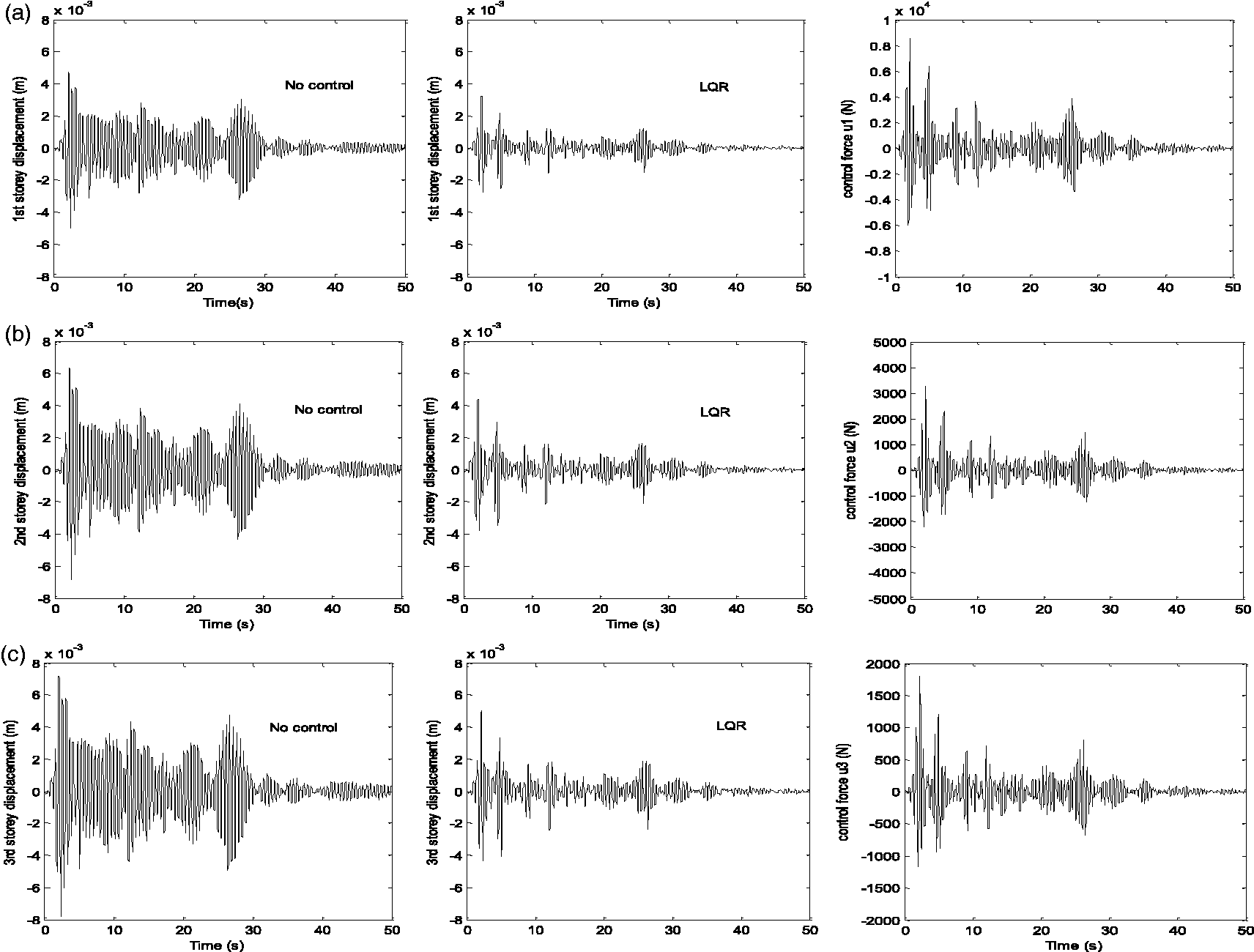
First, the LQR algorithm has been applied to mitigate the structural vibration under Kanai-Tajimi and Clough–Penzien earthquake. This controller has been calculated using the MIMO structural model. Then, the LQR controllers, using the empirical model, have been calculated to each story of the structure. In this case, we calculate the decoupled model by ignoring the interaction term (ϕi*). So we can obtain a mono-variable linear time varying system for each story for the structure.
We have compared all the controller performances with the Empirical GMV control algorithm proposed in this paper. The LQR algorithm proposed (see section LQR algorithm)has presented weak performances compared to our approach. In fact, the results show the superiority of the empirical approach as presented in Tables 2 to 7 and Figures 11 to 20.
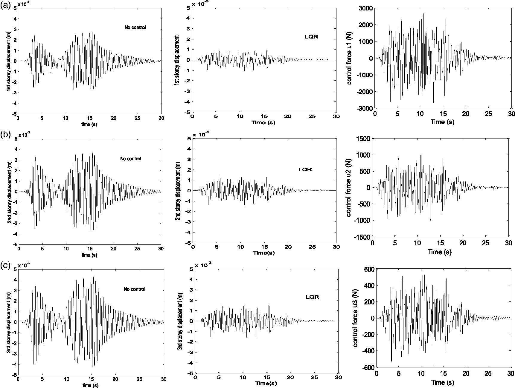
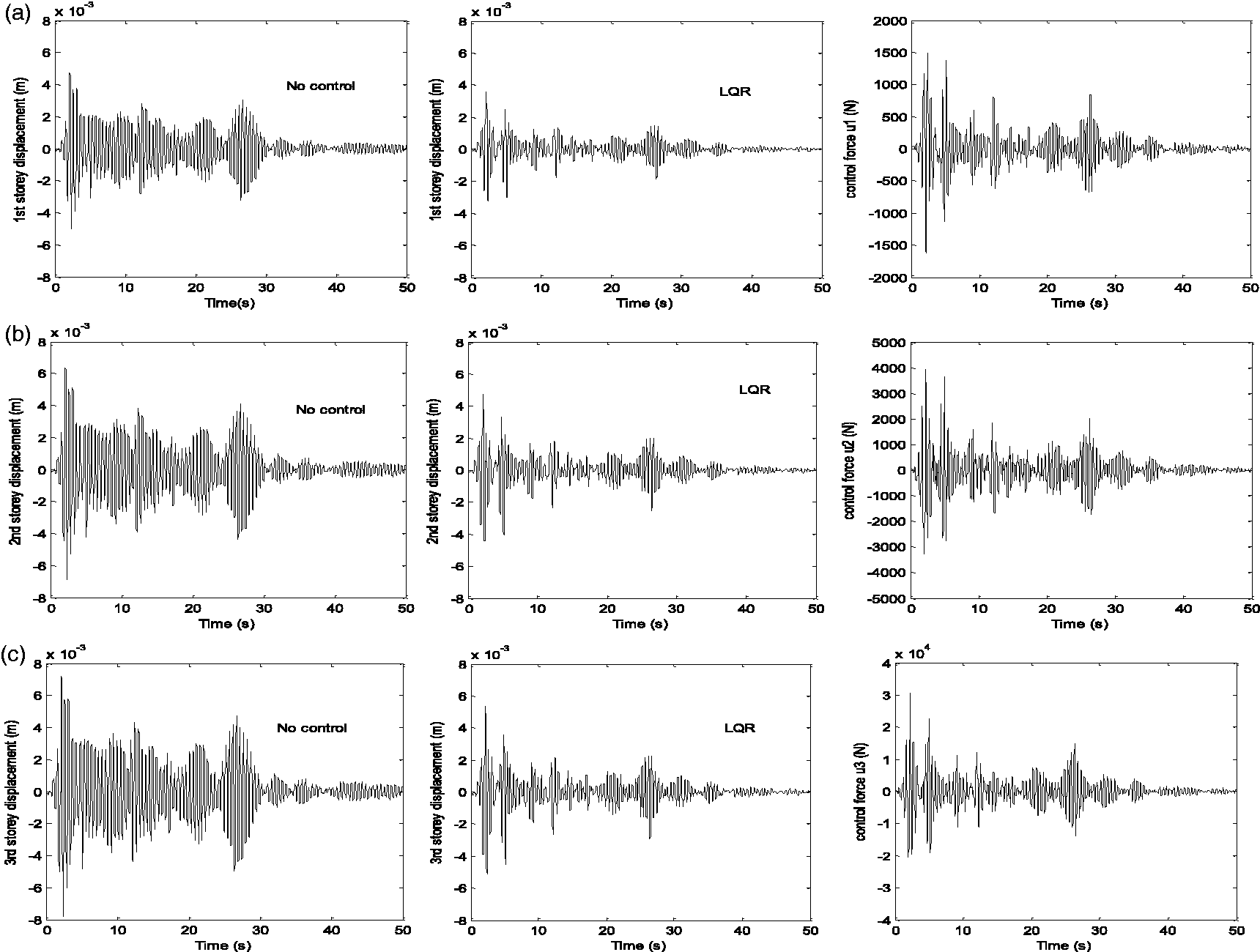
LQR approach: structural response to Clough–Penzien ground acceleration. LQR: linear quadratic regulator.
LQR approach: structural response to Kanai-Tajimi ground acceleration. LQR: linear quadratic regulator.
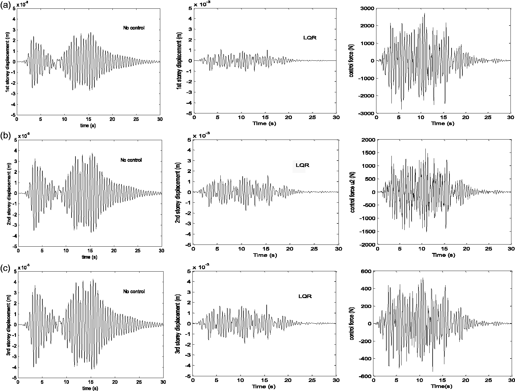
Empirical LQR approach: structural response to Kanai-Tajimi ground acceleration. LQR: linear quadratic regulator.
Empirical LQR approach: structural response to Clough–Penzien ground acceleration. LQR: linear quadratic regulator.
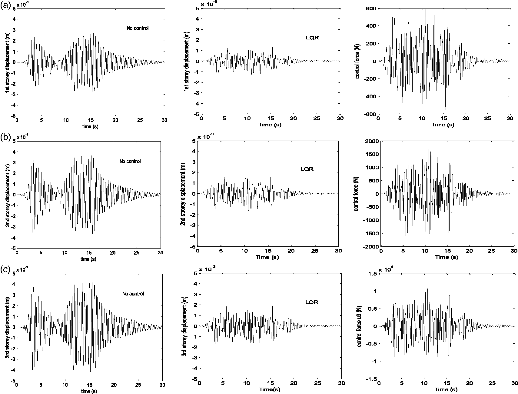
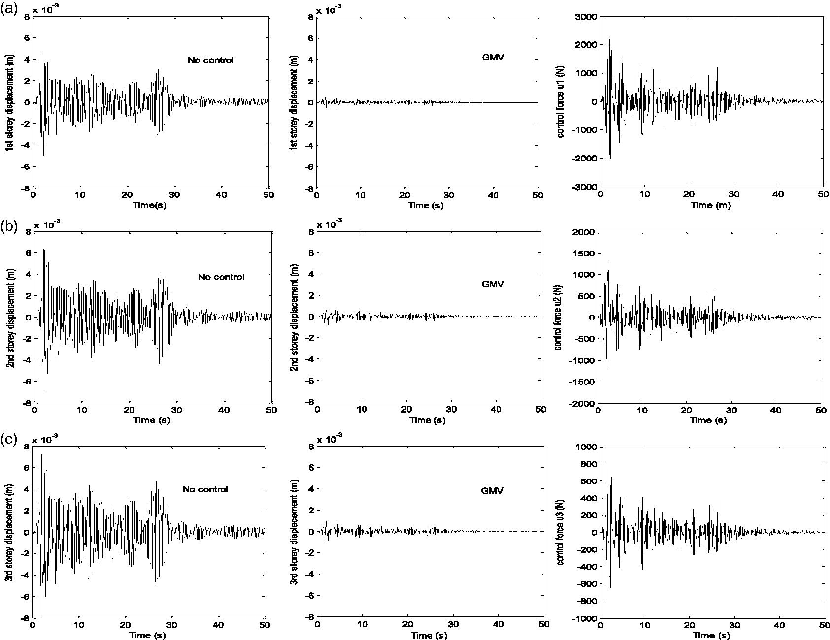
GMV approach: structural response to Kanai-Tajimi ground acceleration. GMV: generalized minimum variance.
GMV approach: structural response to Clough–Penzien ground acceleration.

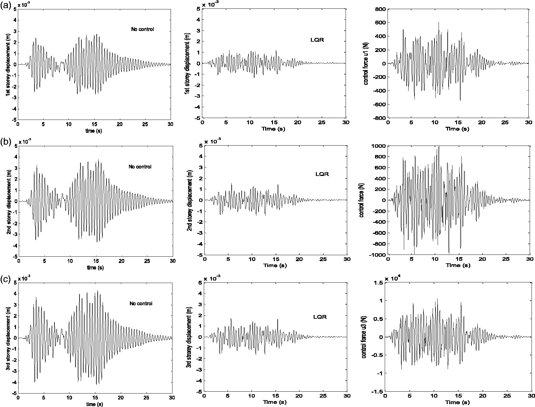
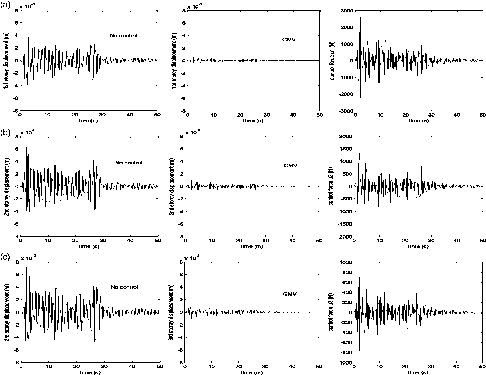
Empirical GMV approach: structural response to Kanai-Tajimi ground acceleration. GMV: generalized minimum variance.
Empirical GMV approach: structural response to Clough–Penzien ground acceleration. GMV: generalized minimum variance.
LQR approach: structural response to EL Centro Earthquake.
Empirical LQR approach: structural response to El Centro Earthquake. LQR: linear quadratic regulator.
GMV approach: structural response to EL Centro Earthquake. GMV: generalized minimum variance.
Empirical GMV approach: structural response to EL Centro Earthquake. GMV: generalized minimum variance.
Output variance.
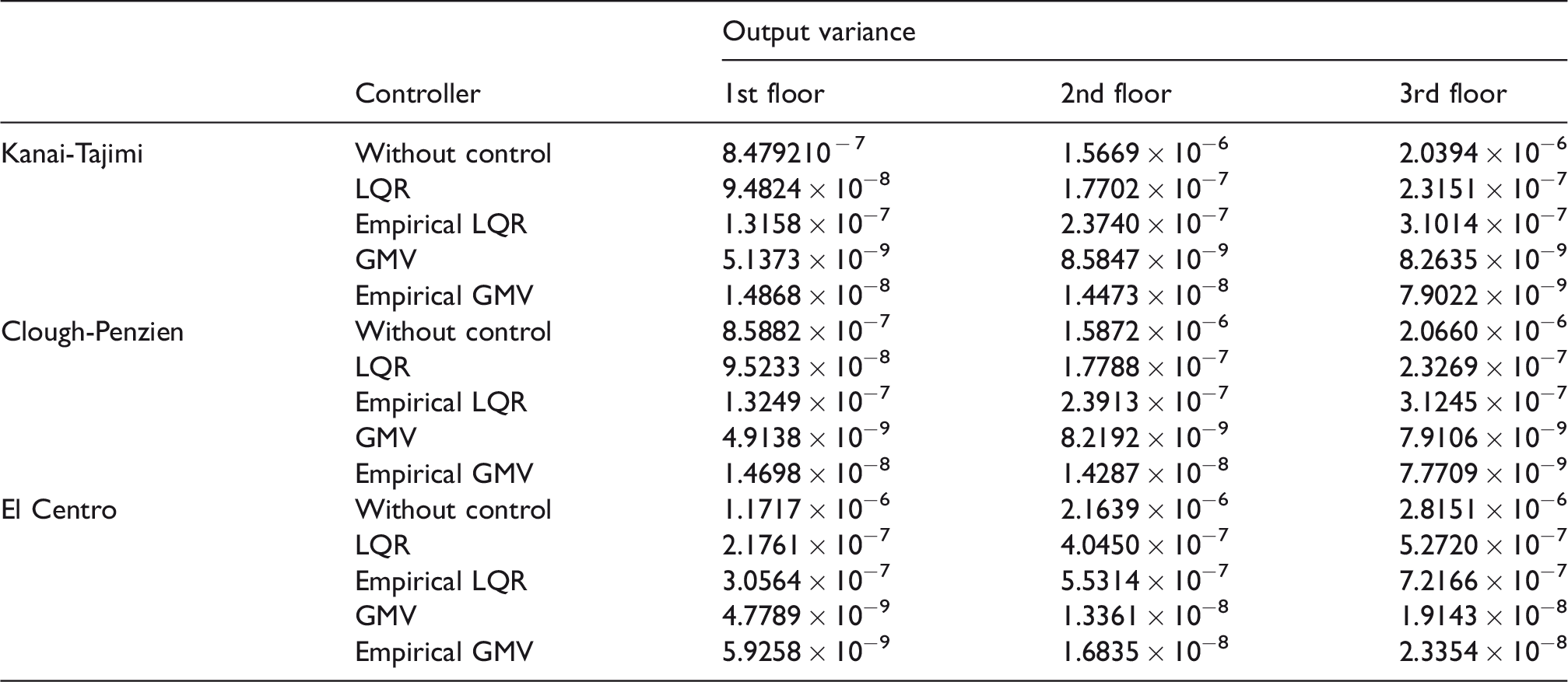
LQR: linear quadratic regulator; GMV: generalized minimum variance.
Maximum displacement.
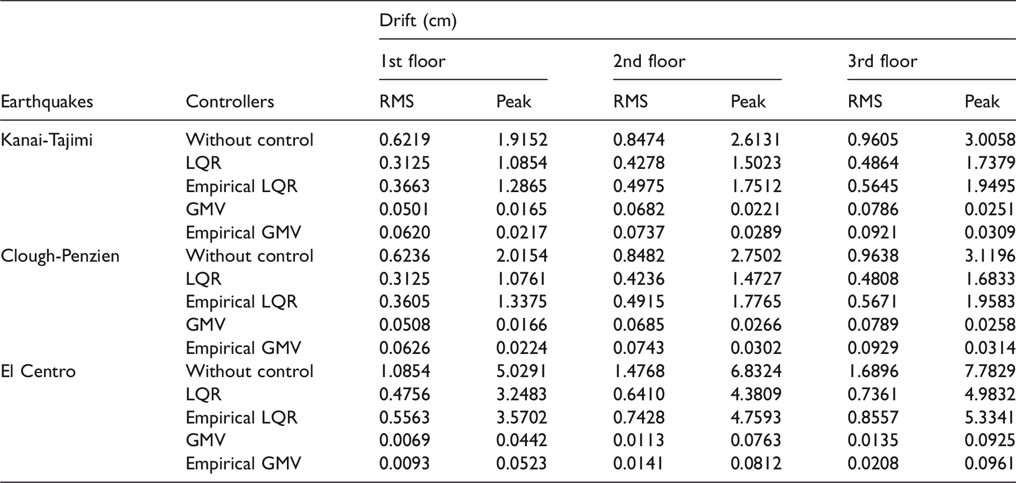
LQR: linear quadratic regulator; GMV: generalized minimum variance.
Maximum acceleration.
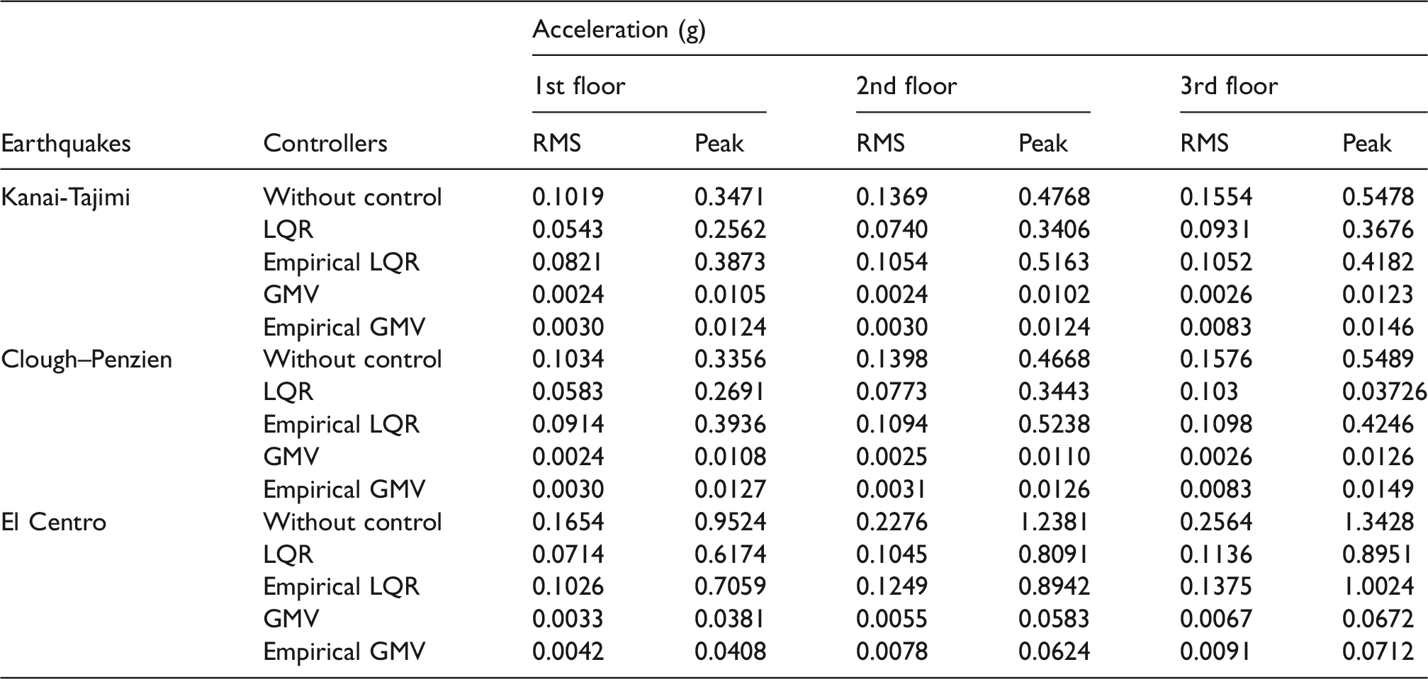
LQR: linear quadratic regulator; GMV: generalized minimum variance.
Maximum control effort.
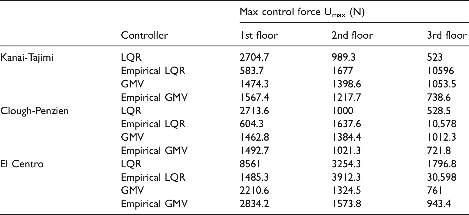
LQR: linear quadratic regulator; GMV: generalized minimum variance.
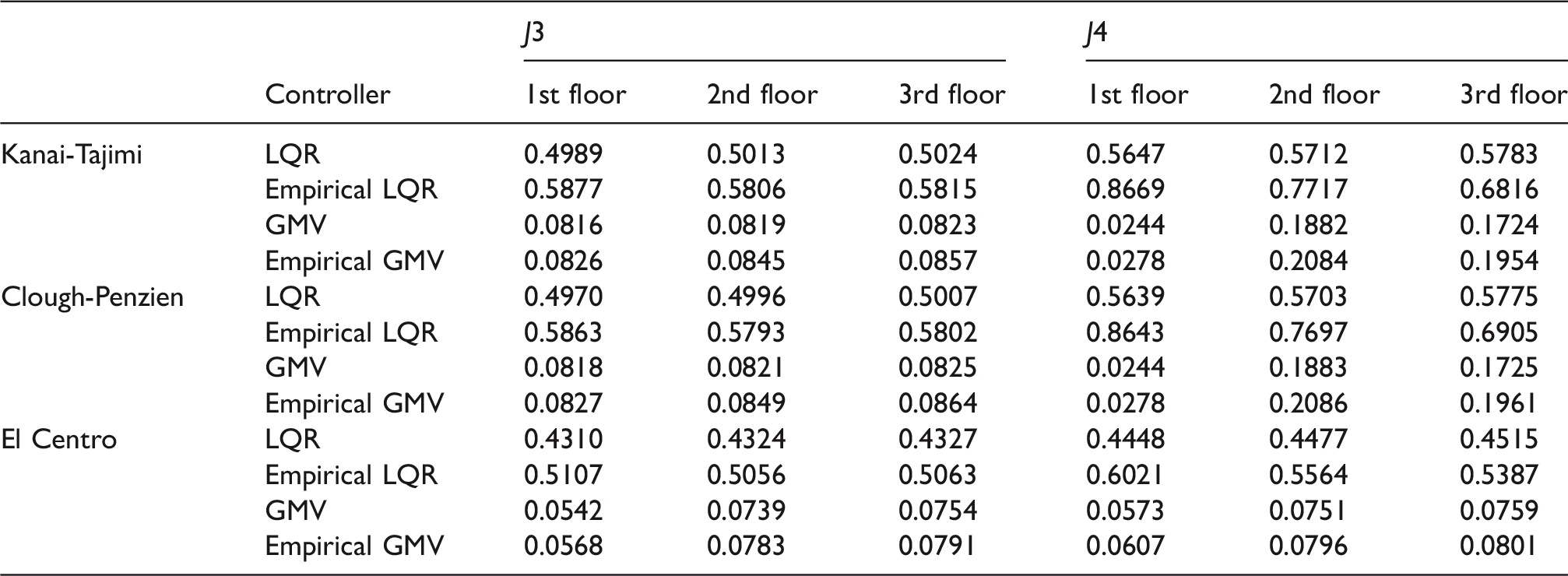
Responses and accelerations ratios (evaluation criteria).
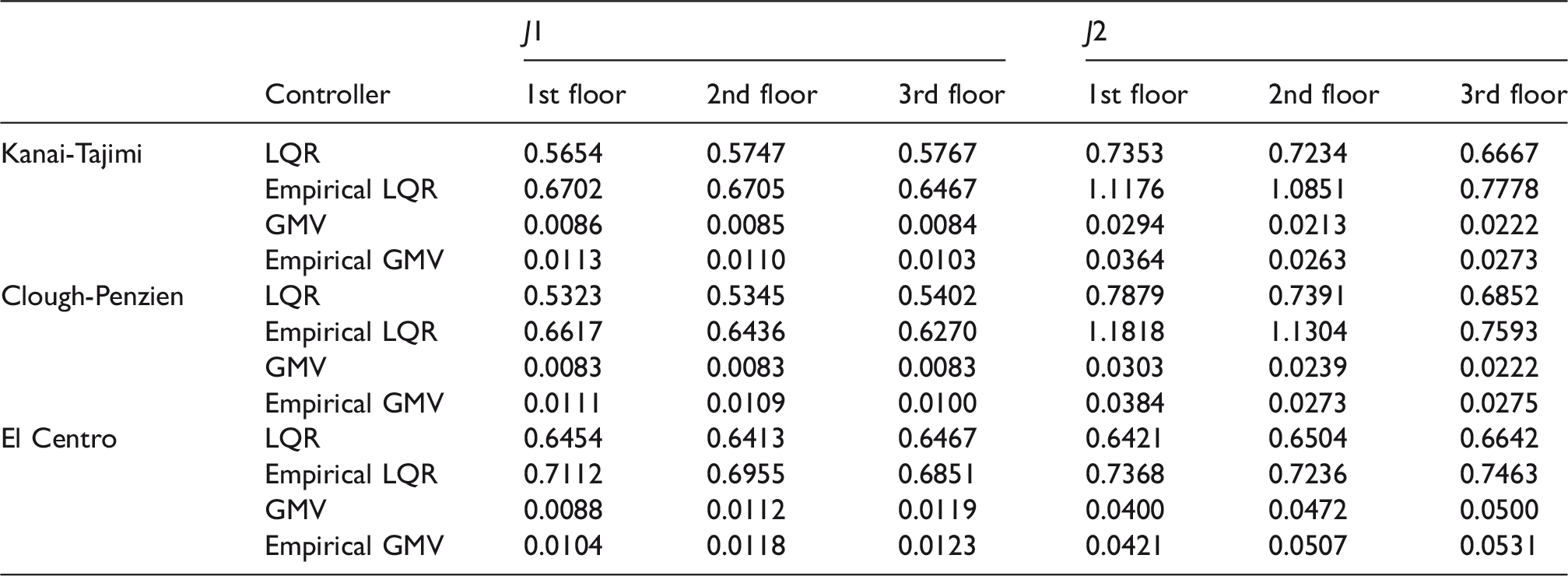
LQR: linear quadratic regulator; GMV: generalized minimum variance.
RMS responses and acceleration ratios (evaluation criteria).
LQR: linear quadratic regulator; GMV: generalized minimum variance ; RMS : root mean square.
On the other hand, we have proposed the GMV control algorithm for MDOF structure under earthquake. This controller was developed based on the ARMAX model calculation using the MIMO structural model. The GMV controller has shown its efficiency.
The Empirical GMV method has been compared to the MDOF GMV algorithm. The results have shown the robustness of the proposed method as presented in Tables 2 to 7 and Figures 11 to 22.
Simulation results show the effectiveness of the control approach. Structural responses are significantly reduced with an acceptable control effort. Indeed, the deep comparison made in this paper has shown a small advantage for the multivariable case over the empirical approach. This result is logical because the MIMO case takes the interconnection terms into account in the control law calculation which brings more suitable performances. On the other hand, even if the interconnection terms are considered as external perturbations, the empirical approach has shown very satisfying results (very close to MIMO GMV results) using a simplified structural modal with less complicated control law calculations. On the other hand, the GMV controller has shown good robustness for compensating the external perturbations
For comparison purposes, Table 2 gives the output variance for each story.
To highlight the controllers performances, the displacement Peak, the RMS and the control effort peak of each controller of each story of the structures under different earthquakes are presented in Tables 3 to 5.
To evaluate the control algorithm performances, the following evaluation criteria are adopted from literature.28–31 are considered.
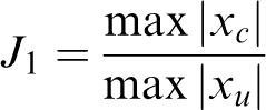
Story displacement ratio
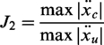
Story acceleration ratio
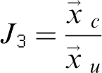
Root mean square (RMS) story displacement ratio

Ts is the sampling time.
Tf is the total excitation duration.std is the standard deviation.
RMS story acceleration ratio

Tables 6 and 7 show the reduction in the peak story displacement without control compared with the proposed control algorithms.
Conclusions
This paper investigated the GMV control algorithm applied to earthquake excited MDOF structures. The control approach was developed and presented based on an empirical model. Our approach has given good performances and the structural responses are significantly reduced. This approach is an extension to the mono-variable case of the classical GMV algorithm. It is designed for the structure as a multivariable system based on local GMV controllers.
Simulation results have shown that our method (the empirical approach) is efficient, despite the fact that this approach does not consider the interaction effects between story units.
It has been shown that the multivariable model is complicated with a well-established theoretical development. In fact, the MIMO case has the disadvantage of the great amount of calculations and matrix manipulation especially in the case of tall buildings with a large number of degrees of freedom. However, our approach has the advantage of presenting a decentralized system. Each local GMV controller can be implemented in local computer hardware which reduces significantly time calculations and memory requirements.
Footnotes
Declaration of conflicting interests
The author(s) declared no potential conflicts of interest with respect to the research, authorship, and/or publication of this article.
Funding
The author(s) received no financial support for the research, authorship, and/or publication of this article.