An explicit formula of perturbating stiffness matrix for partial natural frequency assignment using static output feedback

Abstract

The partial eigenvalue (or natural frequency) assignment or placement, only by the stiffness matrix perturbation, of an undamped vibrating system is addressed in this paper. A novel and explicit formula of determining the perturbating stiffness matrix is deduced from the eigenvalues perturbation theorem for a low-rank perturbed matrix. This formula is then utilized to solve the partial eigenvalue (or natural frequency) assignment via the static output feedback. The control matrix, output matrix and feedback gain matrix can be explicitly expressed and easily constructed.

Introduction

In the last dozen years, the partial eigenvalue (or natural frequency) assignment or placement has been a rich research area. Many aspects of the inverse problem of structural and mechanical dynamics have been involved in the research, such as the structural inverse modification,^1–3 model updating^4–6 and active vibration control.^7–12 These cited here are a small part of the literatures published in recent years. In the above research content, the proposed methods have a nice feature, that is, all the unassigned eigenvalues (or unmodified natural frequencies) with the corresponding eigenvectors remain unchanged while a small number of eigenvalues of a structure are assigned to the targeted values. The results and related methods with this feature are also deemed to be no spillover.

This paper is concerned with the partial eigenvalue (or natural frequency) assignment or placement, only by the stiffness matrix perturbation, of an undamped vibrating system. A novel and simple formula is presented for determining the perturbating stiffness matrix. It is derived from the important results given by Brauer and the others,^13,14 who proved the eigenvalues perturbation theorem for a low-rank perturbed matrix. The application of the formula is then explored in dealing with some related aspects mentioned above, especially in solving the static output feedback control of an undamped vibrating system.

The Brauer’s theorem and a related result

The relationship among eigenvalues of a given square matrix A and its rank one updated matrix was proved by Brauer. ¹³ The following Theorem 2 is an extension of the Brauer’s theorem. Firstly, the Brauer’s theorem is introduced as follows.

Theorem 1.^13,15 Let A be an n × n arbitrary matrix with eigenvalues $\{{\text{λ}}_1,{\text{λ}}_2,\mathrm{\dots }\mathrm{\hspace{0.17em}},{\text{λ}}_n\}$ . Let $x_k$ be an eigenvector of A associated with the eigenvalue ${\text{λ}}_k$ , and let $u$ be any n-dimensional column vector. Then, the matrix $\text{A}+x_k{u}^T$ has eigenvalues $\{{\text{λ}}_1,\mathrm{\dots }\mathrm{\hspace{0.17em}},{\text{λ}}_{k-1},{\text{λ}}_k+x_k^{T}u, {\text{λ}}_{k+1},\mathrm{\dots }\mathrm{\hspace{0.17em}},{\text{λ}}_n\}$ .

Theorem 1 shows that eigenvalues of the matrix $\text{A}+x_k{u}^T$ consist of those of A, except that one eigenvalue ${\text{λ}}_k$ of A is replaced by ${\text{λ}}_k+x_k^{T}u$ . The following theorem further describes how to modify, in only one step, r eigenvalues of an arbitrary square matrix A without changing any of the remaining (n − r) eigenvalues.

Theorem 2.^14,15 Let A be an n × n arbitrary matrix with eigenvalues $\{{\text{λ}}_1,{\text{λ}}_2,\mathrm{\dots }\mathrm{\hspace{0.17em}},{\text{λ}}_n\}$ . Let ${\text{X}}_1=\left[x_1{x}_2\mathrm{\dots } x_r\right]$ be an n × r matrix such that rank(X₁) = r and $\text{A}{x}_i={\text{λ}}_i{x}_i$ , i = 1, 2, …, r, $r\le n$ . Let C be an r × n arbitrary matrix. Then, the matrix $\text{A}+{\text{X}}_1\text{C}$ has eigenvalues $\left\{{\mu }_1,{\mu }_2,\mathrm{\dots }\mathrm{\hspace{0.17em}},{\mu }_r,{\text{λ}}_{r+1},{\text{λ}}_{r+2},\mathrm{\dots }\mathrm{\hspace{0.17em}},{\text{λ}}_n\right\}$ , where ${\mu }_1,{\mu }_2,\mathrm{\dots }\mathrm{\hspace{0.17em}},{\mu }_r$ are eigenvalues of the matrix ${\text{Λ}}_1+{\text{CX}}_1$ with ${\text{Λ}}_1=\text{diag}\left({\text{λ}}_1,{\text{λ}}_2,\mathrm{\dots }\mathrm{\hspace{0.17em}},{\text{λ}}_r\right)$ .

In the next section only the stiffness matrix perturbation of a vibrating system is considered. The aim is to assign some natural frequencies of the original system with no spillover. A new explicit formula of the perturbating stiffness matrix will be presented based on above Theorem 2. Its computation is fairly straightforward when changing amounts of some natural frequencies of the original system are given.

An explicit formula of the perturbating stiffness matrix

Consider an n-degree-of-freedom undamped vibrating system that is modeled by the following set of homogeneous second-order ordinary differential equations

$${\text{M}}_0\ddot{q}\left(t\right)+{\text{K}}_{0}q(t)=0$$

(1)

where $q(t)$ is n-dimensional displacement vector depending on time t, ${\text{M}}_0,{\text{K}}_0$ are n × n mass and stiffness matrices, respectively. In general, ${\text{M}}_{0 }$ is symmetric and positive definite, and ${\text{K}}_0$ is symmetric and positive semi-definite, denoted by ${\text{M}}_0>0$ , ${\text{K}}_0\ge 0$ . It is well known that dynamical performances of the system (1) are characterized by the following generalized eigenvalue equations

$${\text{K}}_0{x}_i={\lambda }_i{\text{M}}_0{x}_i,i=1,2,\dots ,n$$

(2)

where ${\lambda }_i={\omega }_i^2$ is the square of the ith natural frequency ${\omega }_i$ , called the ith eigenvalue and $x_i$ is the corresponding ith mode shape, called the ith eigenvector.

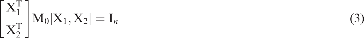
The real number set of eigenvalues of the system (1) can be partitioned into two non-intersection subsets $\{{\text{λ}}_1,{\text{λ}}_2,\mathrm{\dots }\mathrm{\hspace{0.17em}},{\text{λ}}_r\}$ and $\{{\text{λ}}_{\text{r}+1},{\text{λ}}_{\text{r}+2},\mathrm{\dots }\mathrm{\hspace{0.17em}},{\text{λ}}_n\}$ . For the convenience of the following exposition, the former subset and the corresponding eigenvectors are expressed by, respectively, two submatrices, that is ${\text{Λ}}_1=\text{diag}\left({\text{λ}}_1,{\text{λ}}_2,\mathrm{\dots }\mathrm{\hspace{0.17em}},{\text{λ}}_r\right)$ and ${\text{X}}_1=\left[x_1{x}_2\mathrm{\dots } x_r\right]$ , which are consistent with the expression in Theorem 2. The latter subset and the corresponding eigenvectors are represented by ${\text{Λ}}_2=\text{diag}\left({\text{λ}}_{r+1},{\text{λ}}_{r+2},\mathrm{\dots }\mathrm{\hspace{0.17em}},{\text{λ}}_n\right)$ and ${\text{X}}_2=\left[x_{r+1}{x}_{r+2}\mathrm{\dots } x_n\right]$ . Additionally, it is always assumed without loss of generality that the eigenvectors ( ${\text{X}}_1$ , ${\text{X}}_2$ ) of the system (1) are normalized in such a way that

$$\left[\begin{array}{c}{\text{X}}_1^{\text{T}}\\ {\text{X}}_2^{\text{T}}\end{array}\right]{\text{M}}_0\left[{\text{X}}_1,{\text{X}}_2\right]={\text{I}}_n$$

(3)

$$\left[\begin{array}{c}{\text{X}}_1^{\text{T}}\\ {\text{X}}_2^{\text{T}}\end{array}\right]{\text{K}}_0\left[{\text{X}}_1,{\text{X}}_2\right]=\text{diag}\left({\text{Λ}}_1,{\text{ Λ}}_2\right)$$

(4)

where the superscript T denotes the matrix transpose, and ${\text{I}}_n$ is an n × n identity matrix.

Now the problem is to change the eigenvalues subset $\{{\text{λ}}_1,{\text{λ}}_2,\mathrm{\dots }\mathrm{\hspace{0.17em}},{\text{λ}}_r\}$ of the system (1) to another subset of targeted eigenvalues $\{{\mu }_1,{\mu }_2,\mathrm{\dots }\mathrm{\hspace{0.17em}},{\mu }_r\}$ , which is also written as a submatrix ${\text{Σ}}_1=\text{diag}\left({\mu }_1,{\mu }_2,\mathrm{\dots }\mathrm{\hspace{0.17em}},{\mu }_r\right)$ , while keeping any of the remaining (n − r) eigenvalues $\{{\text{λ}}_{\text{r}+1},{\text{λ}}_{\text{r}+2},\mathrm{\dots }\mathrm{\hspace{0.17em}},{\text{λ}}_n\}$ and the corresponding eigenvectors of the system (1) unchanged. Furthermore, that’s all going to be done through only replacing or updating the stiffness matrix ${\text{K}}_0$ by ${\text{K}}_0+\text{ΔK}$ in the system (1). Notice that an assumption, $\left\{{\mu }_1,{\mu }_2,\mathrm{\dots }\mathrm{\hspace{0.17em}},{\mu }_r\right\}\cap \left\{{\text{λ}}_{\text{r}+1},{\text{λ}}_{\text{r}+2},\mathrm{\dots }\mathrm{\hspace{0.17em}},{\text{λ}}_n\right\}=\varnothing$ , is made in this problem. In what follows, the perturbating stiffness matrix $\text{ΔK}$ is constructively presented for solving the problem.

The generalized eigenproblem (2) can be equivalently transformed into a standard eigenproblem via letting $\text{A}={\text{M}}_0^{-1}{\text{K}}_0$ . It follows from Theorem 2 that, if the matrix ${\text{Λ}}_1+{\text{CX}}_1$ has eigenvalues $\left\{{\mu }_1,{\mu }_2,\mathrm{\dots }\mathrm{\hspace{0.17em}},{\mu }_r\right\}$ , then $\text{A}+{\text{X}}_1\text{C}={\text{M}}_0^{-1}{\text{K}}_0+{\text{X}}_1\text{C}$ has eigenvalues $\left\{{\mu }_1,{\mu }_2,\mathrm{\dots }\mathrm{\hspace{0.17em}},{\mu }_r,{\text{λ}}_{r+1},{\text{λ}}_{r+2},\mathrm{\dots }\mathrm{\hspace{0.17em}},{\text{λ}}_n\right\}$ , noting that $\text{C}$ is an r × n arbitrary matrix. Let $\text{C}=\left({\text{Σ}}_1-{\text{Λ}}_1\right){\text{X}}_1^{\text{T}}{\text{M}}_0$ , since ${\text{X}}_1^{\text{T}}{\text{K}}_0{\text{X}}_1={\text{Λ}}_1$ and ${\text{X}}_1^{\text{T}}{\text{M}}_0{\text{X}}_1={\text{I}}_r$ from (equations (3) and 4), it is easy to verify that

$${\text{Λ}}_1+{\text{CX}}_1={\text{X}}_1^{\text{T}}{\text{K}}_0{\text{X}}_1+\left({\text{Σ}}_1-{\text{Λ}}_1\right){\text{X}}_1^{\text{T}}{\text{M}}_0{\text{X}}_1={\text{Σ}}_1=\text{diag}\left({\mu }_1,{\mu }_2,\mathrm{\dots }\mathrm{\hspace{0.17em}},{\mu }_r\right)$$

Thus, $\text{A}+{\text{X}}_1\text{C}={\text{M}}_0^{-1}{\text{K}}_0+{\text{X}}_1\text{C}={\text{M}}_0^{-1}{\text{K}}_0+{\text{X}}_1\left({\text{Σ}}_1-{\text{Λ}}_1\right){\text{X}}_1^{\text{T}}{\text{M}}_0$ has eigenvalues $\left\{{\mu }_1,{\mu }_2,\mathrm{\dots }\mathrm{\hspace{0.17em}},{\mu }_r,{\text{λ}}_{r+1},{\text{λ}}_{r+2},\mathrm{\dots }\mathrm{\hspace{0.17em}},{\text{λ}}_n\right\}$ . Premultiplying the matrix ${\text{M}}_0^{-1}{\text{K}}_0+{\text{X}}_1\left({\text{Σ}}_1-{\text{Λ}}_1\right){\text{X}}_1^{\text{T}}{\text{M}}_0$ with ${\text{M}}_0$ , then the standard eigenproblem of this matrix can be equivalently transformed into the following generalized eigenproblem

$$({\text{K}}_0+\text{ΔK})y_i={\mu }_i{\text{M}}_0{y}_i,i=1,2,\dots ,r$$

(5a)

and

$$({\text{K}}_0+\text{ΔK})y_j={\text{λ}}_j{\text{M}}_0{y}_j,j=r+1,r+2,\dots ,n$$

(5b)

where

$$\text{ΔK}={\text{M}}_0{\text{X}}_1\left({\text{Σ}}_1-{\text{Λ}}_1\right){\text{X}}_1^{\text{T}}{\text{M}}_0$$

(6)

In this case, it can also be shown from Proposition 5 of Bru et al. ¹⁵ that the eigenvectors associated with the eigenvalues $\left\{{\text{λ}}_{r+1},{\text{λ}}_{r+2},\mathrm{\dots }\mathrm{\hspace{0.17em}},{\text{λ}}_n\right\}$ for the eigenproblem (5) and (2) are the same. Thus, the aforementioned problem is solved with equation (6).

Remark 1: (i) $\text{ΔK}$ with equation (6) is exactly symmetrical, and eigenvectors associated with eigenvalues $\{{\text{λ}}_1,{\text{λ}}_2,\mathrm{\dots }\mathrm{\hspace{0.17em}},{\text{λ}}_r\}$ of the eigenproblem (2) are also the eigenvectors associated with the eigenvalues $\left\{{\mu }_1,{\mu }_2,\mathrm{\dots }\mathrm{\hspace{0.17em}},{\mu }_r\right\}$ of the eigenproblem (5). This can be concluded from Proposition 4 of Bru et al. ¹⁵ (ii) In Chu et al. ¹⁶ authors discussed the one-sided updating, that is the stiffness matrix updating, for model updating of the system (1) with no spillover. They had proved that any feasible candidate $\text{ΔK}$ must be parameterized form of $\text{ΔK}={\text{M}}_0{\text{X}}_1{\text{ΦX}}_1^{\text{T}}{\text{M}}_0$ , where $\text{Φ}$ is a parametric symmetric matrix. In this paper, the simplest form of $\text{ ΔK}$ is provided for partial eigenvalue (or natural frequency) assignment or placement. Its computation is a simple one-step procedure, and no extra eigen-matrix equation is needed to solve for $\text{Φ}$ as required in Chu et al. ¹⁶ (iii) For some real generalized eigenproblem, that is Ax =  $\text{λ}$ Bx with A, B being real matrices and B > 0, if all of its eigenvalues are non-defective, the similar result as equation (6) in the paper can also be obtained for partial eigenvalue assignment or placement via the perturbation of matrix A.

Applications of the formula

In this section, the main application of the formula (6) dedicated to the static output feedback control is discussed. Notice that directly updating stiffness matrix from measured natural frequencies using the formula (6) is a rather trivial matter and the updated model is no spillover.

When considering the external applied forces that come from the static output feedback control, the motion equations of the system (1) can be rewritten as

$${\text{M}}_0\ddot{q}\left(t\right)+{\text{K}}_{0}q(t)=\text{B}u\left(t\right)$$

(7a)

$$u\left(t\right)=-\text{G}\nu (t)$$

(7b)

$$\nu \left(t\right)=\text{C}q(t)$$

(7c)

where B is a constant n × m control matrix, C a constant m × n output matrix, G a constant output feedback gain matrix to be determined and $m<n$ . $u\left(t\right)$ is the control forces vector, $\nu \left(t\right)$ the output or measurement vector. An assumption that both $u\left(t\right)$ and $\nu \left(t\right)$ are m-dimensional vector is made here. Substituting equations (7b) and (7c) into equation (7a), then the closed-loop motion equations of the system (1) becomes

$${\text{M}}_0\ddot{q}\left(t\right)+\left({\text{K}}_0+\text{BGC}\right)q(t)=0$$

(8)

and the associated generalized eigenproblem is given as

$$({\text{K}}_0+\text{BGC})y_i={\mu }_i{\text{M}}_0{y}_i,i=1,2,\dots ,n$$

(9)

Letting $m=r$ , comparing equation (9) with equation (5) gives

$$\text{ΔK}={\text{M}}_0{\text{X}}_1\left({\text{Σ}}_1-{\text{Λ}}_1\right){\text{X}}_1^{\text{T}}{\text{M}}_0=\text{BGC}$$

(10)

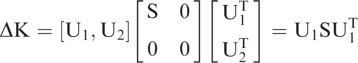
Now an approach to solve the partial eigenvalues (or natural frequencies) assignment of the system (1) via the static output feedback is presented. For the case of collocated actuator and sensor pairs with $\text{C}={\text{B}}^{\text{T}}$ , letting $\text{B}={\text{M}}_0{\text{X}}_1$ , $\text{C}={\text{X}}_1^{\text{T}}{\text{M}}_0$ and $\text{G}={\text{Σ}}_1-{\text{Λ}}_1$ , then a specific solution is easily achieved. Another specific solution deserves to be considered, which can be obtained from the singular value decomposition (SVD) of $\text{ΔK}$ .

$$\text{ΔK}=\left[{\text{U}}_1,{\text{U}}_2\right]\left[\begin{array}{cc}\text{S}& 0\\ 0& 0\end{array}\right]\left[\begin{array}{c}{\text{U}}_1^{\text{T}}\\ {\text{U}}_2^{\text{T}}\end{array}\right]={\text{U}}_1{\text{SU}}_1^{\text{T}}$$

Thus, it is obvious that $\text{B}={\text{U}}_1$ , $\text{C}={\text{U}}_1^{\text{T}}$ and $\text{G}=\text{S}$ .

Moreover, the following parameterized solutions can be proposed through rewriting equation (10) as

$${\text{M}}_0{\text{X}}_1\varphi {\varphi }^{-1}\left({\text{Σ}}_1-{\text{Λ}}_1\right){\varphi }^{-1}\varphi {\text{X}}_1^{\text{T}}{\text{M}}_0=\text{BGC}$$

(11)

where $\varphi$ is an m × m arbitrary, non-singular symmetric matrix. In this case, the solutions are

$$\text{B}={\text{M}}_0{\text{X}}_1\varphi$$

(12a)

$$\text{C}=\varphi {\text{X}}_1^{\text{T}}{\text{M}}_0$$

(12b)

and

$$\text{G}={\varphi }^{-1}\left({\text{Σ}}_1-{\text{Λ}}_1\right){\varphi }^{-1}$$

(12c)

For the case of non-collocated actuators and sensors configuration with $\text{C}\ne \text{B}$ , rewriting equation (10) as

$${\text{M}}_0{\text{X}}_1{\varphi }_1{\varphi }_1^{-1}\left({\text{Σ}}_1-{\text{Λ}}_1\right){\varphi }_2^{-1}{\varphi }_2{\text{X}}_1^{\text{T}}{\text{M}}_0=\text{BGC}$$

(13)

where ${\varphi }_1$ , ${\varphi }_2$ are m × m arbitrary, non-singular matrices, then the parameterized solutions are

$$\text{B}={\text{M}}_0{\text{X}}_1{\varphi }_1$$

(14a)

$$\text{C}={\varphi }_2{\text{X}}_1^{\text{T}}{\text{M}}_0$$

(14b)

and

$$\text{G}={\varphi }_1^{-1}\left({\text{Σ}}_1-{\text{Λ}}_1\right){\varphi }_2^{-1}$$

(14c)

Remark 2: (i) $\text{B}$ , $\text{ C}$ and $\text{G}$ obtained here preserve the symmetry and the positive semi-definiteness of the open-loop system (1) after feedback, regardless of collocated or non-collocated configuration of actuators and sensors. The symmetry, definiteness and reciprocity property of second-order systems are highly significant from practical application view point, which involve the stability, computation algorithms and test methods of considered systems.^2,4,17 For vibroacoustical coupled problems, the vibroacoustical reciprocity principle is also valid, although the second-order model formulation describing vibroacoustical coupling is a non-symmetrical matrix equation. ¹⁸ (ii) The control influence matrix B and the output measurement matrix C in this paper are most likely to be dense matrices. But due to the recent progress of the smart materials with distributed arrays of transducers the application of dense matrices B and C can be made feasible. ¹⁹ (iii) If $\text{B }$ and $\text{C}$ are determined a prior for some other considerations, ${\varphi }_1$ , ${\varphi }_2$ (or $\varphi$ ) can be figured out from the linear matrix equations (14a), (14b) (or (12a)). There may be a trial of some adjustment of $\text{B }$ and $\text{C}$ for satisfying the solvability condition of the matrix equations. In practice, ${\varphi }_1$ and ${\varphi }_2$ in equations (14a) and (14b) act as elementary column/row transformations on ${\text{M}}_0{\text{X}}_1$ and ${\text{X}}_1^{\text{T}}{\text{M}}_0$ , respectively.

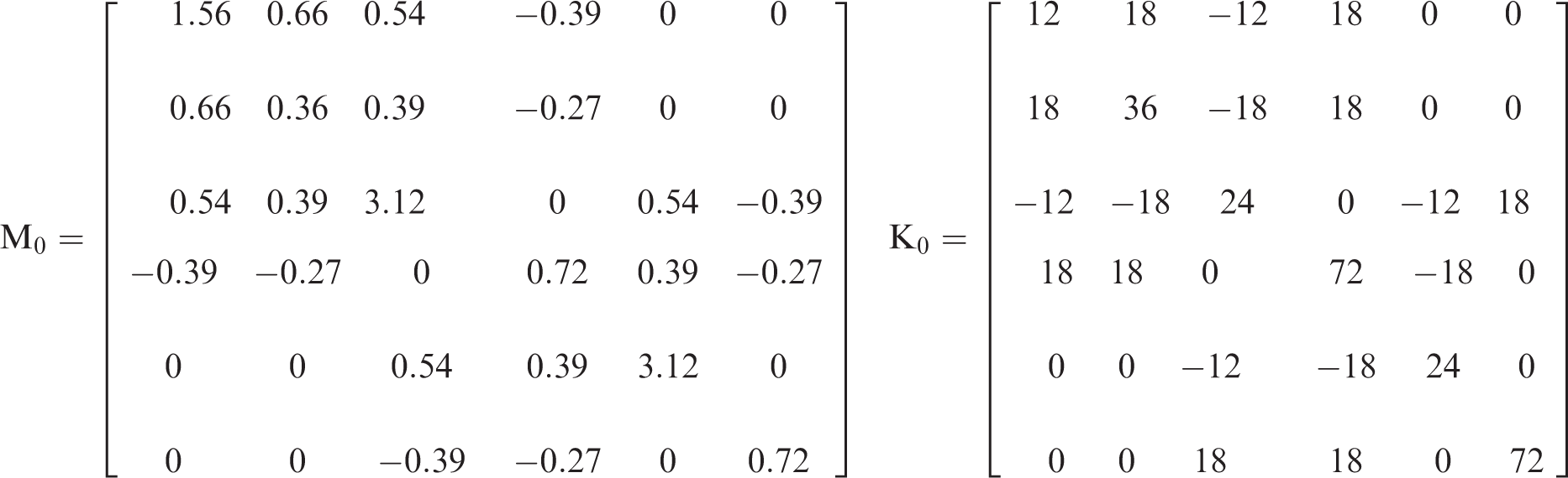
Example 4.1. Consider the system (1) with ${\text{M}}_0$ and ${\text{K}}_0$ as follows

$${\text{M}}_0=\left[\begin{array}{cc}\begin{array}{ccc}1.56& 0.66& 0.54\\ 0.66& 0.36& 0.39\\ 0.54& 0.39& 3.12\end{array}& \begin{array}{ccc}-0.39& 0& 0\\ -0.27& 0& 0\\ 0& 0.54& -0.39\end{array}\\ \begin{array}{ccc}-0.39& -0.27& 0\\ 0& 0& 0.54\\ 0& 0& -0.39\end{array}& \begin{array}{ccc}0.72& 0.39& -0.27\\ 0.39& 3.12& 0\\ -0.27& 0& 0.72\end{array}\end{array}\right]{\text{ K}}_0=\left[\begin{array}{cc}\begin{array}{ccc}12& 18& -12\\ 18& 36& -18\\ -12& -18& 24\end{array}& \begin{array}{ccc}18& 0& 0\\ 18& 0& 0\\ 0& -12& 18\end{array}\\ \begin{array}{ccc}18& 18& 0\\ 0& 0& -12\\ 0& 0& 18\end{array}& \begin{array}{ccc}72& -18& 0\\ -18& 24& 0\\ 18& 0& 72\end{array}\end{array}\right]$$

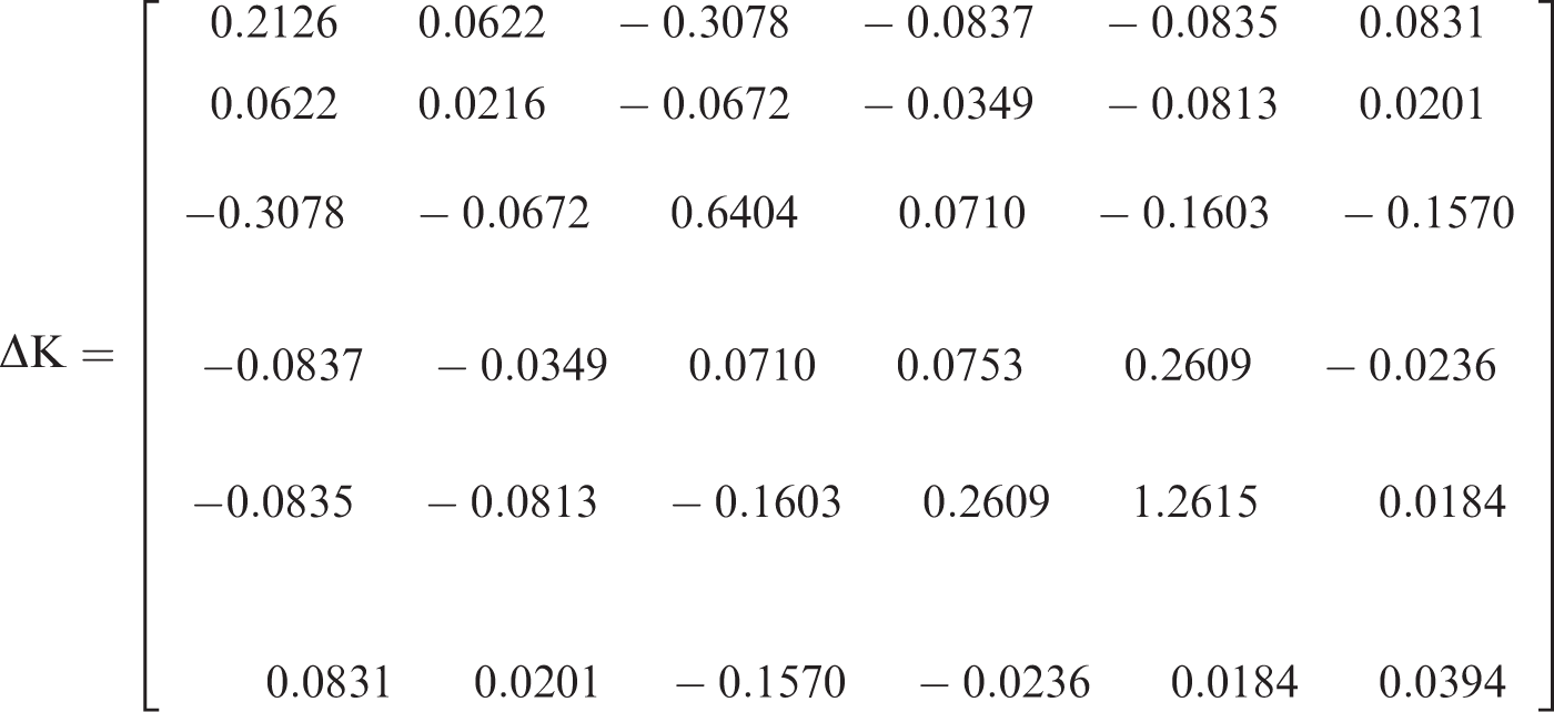
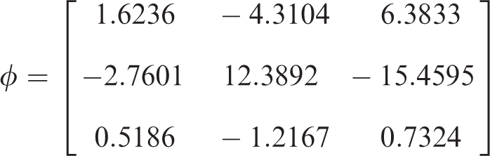
Its eigenvalues are $\left\{0.0364,1.4365,11.4697,58.1668,206.0230,818.8383\right\}$ . Let $r=m=3$ , ${\text{Λ}}_1=\text{diag}\left(0.0364,1.4365,11.4697\right)$ , ${\text{Σ}}_1=\text{diag}\left(0.05,1.8,12\right)$ . ${\text{X}}_1$ associated with ${\text{Λ}}_1$ is not listed for the sake of saving space. From equation (6), it gives

$$\text{ΔK}=\left[\begin{array}{c}0.21260.0622-0.3078-0.0837-0.08350.0831\\ \begin{array}{c}0.06220.0216-0.0672-0.0349-0.08130.0201\\ \begin{array}{c}-0.3078-0.06720.64040.0710-0.1603-0.1570\\ -0.0837-0.03490.07100.07530.2609-0.0236\\ \begin{array}{c}-0.0835-0.0813-0.16030.26091.26150.0184\\ 0.08310.0201-0.1570-0.02360.01840.0394\end{array}\end{array}\end{array}\end{array}\right]$$

The eigenvalues $\left\{0.05,1.8,12.0,58.1668,206.0230,818.8383\right\}$ are those of the perturbed system, which is also no spillover for the corresponding eigenvectors.

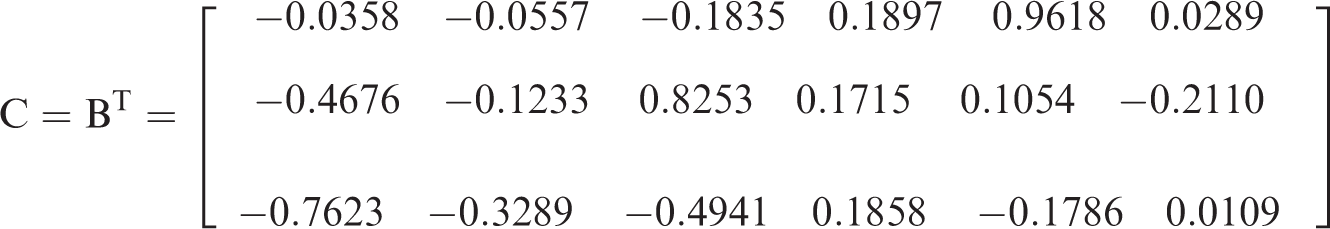
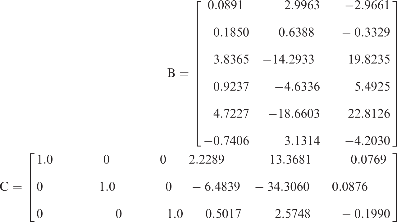
For the collocated configuration, using SVD of above $\text{ΔK}$ gives

$$\text{C}={\text{B}}^{\text{T}}=\left[\begin{array}{c}\begin{array}{ccc}-0.0358& -0.0557& \begin{array}{ccc}-0.1835& 0.1897& \begin{array}{cc}0.9618& 0.0289\end{array}\end{array}\end{array}\\ \begin{array}{c}\begin{array}{ccc}-0.4676& -0.1233& \begin{array}{ccc}0.8253& 0.1715& \begin{array}{cc}0.1054& -0.2110\end{array}\end{array}\end{array}\\ \begin{array}{ccc}-0.7623& -0.3289& \begin{array}{ccc}-0.4941& 0.1858& \begin{array}{cc}-0.1786& 0.0109\end{array}\end{array}\end{array}\end{array}\end{array}\right]$$

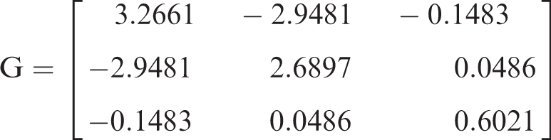
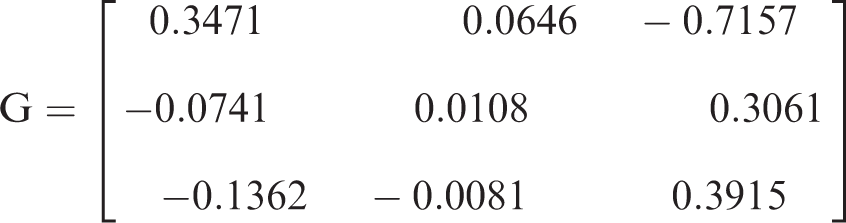
and $\text{G}=\text{diag}\left\{1.3518,0.8593,0.0395\right\}$ . For an arbitrary, nonsingular symmetric matrix $\varphi$ , for example it gives

$$\text{C}={\text{B}}^{\text{T}}=\left[\begin{array}{c}\begin{array}{ccc}1.4417& 0.5986& \begin{array}{ccc}0.2433& -0.5458& \begin{array}{cc}-0.6363& 0.1149\end{array}\end{array}\end{array}\\ \begin{array}{c}\begin{array}{ccc}1.3533& 0.5810& \begin{array}{ccc}0.6019& -0.4488& \begin{array}{cc}-0.2906& 0.0352\end{array}\end{array}\end{array}\\ \begin{array}{ccc}0.4987& 0.1091& \begin{array}{ccc}-0.7357& 0.0349& \begin{array}{cc}1.0287& 0.1944\end{array}\end{array}\end{array}\end{array}\end{array}\right]$$

$$\text{G}=\left[\begin{array}{c}3.2661-2.9481-0.1483\\ -2.94812.68970.0486\\ -0.14830.04860.6021\end{array}\right]$$

where $\varphi =\left[\begin{array}{c}0.81470.90580.1270\\ 0.90580.63240.0975\\ 0.12700.09750.9575\end{array}\right]$

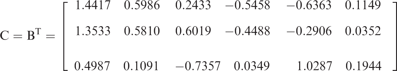
For the non-collocated configuration, let, for example $\varphi ={\varphi }_1={\varphi }_2$ be the transformation matrix of the reduced row echelon form of ${\text{X}}_1^{\text{T}}{\text{M}}_0$ as follows

$$\varphi =\left[\begin{array}{c}1.6236-4.31046.3833\\ -2.760112.3892-15.4595\\ 0.5186-1.21670.7324\end{array}\right]$$

It gives

$$\text{B}=\left[\begin{array}{ccc}0.0891& 2.9963& -2.9661\\ 0.1850& 0.6388& -0.3329\\ 3.8365& -14.2933& 19.8235\\ 0.9237& -4.6336& 5.4925\\ 4.7227& -18.6603& 22.8126\\ -0.7406& 3.1314& -4.2030\end{array}\right]\text{C}=\left[\begin{array}{l}1.0002.228913.36810.0769\hfill \\ 01.00-6.4839-34.30600.0876\hfill \\ 001.00.50172.5748-0.1990\hfill \end{array}\right]$$

$$\text{G}=\left[\begin{array}{c}0.34710.0646-0.7157\\ -0.07410.01080.3061\\ -0.1362-0.00810.3915\end{array}\right]$$

Conclusions

A simple one-step computation formula of the perturbating stiffness matrix is proposed to implement the partial eigenvalue (or natural frequency) assignment or placement. The formula can be used to design the static output feedback control, and to solve the other relevant problems.