Aerodynamic noise radiating from the inter-coach windshield region of a high-speed train

Abstract

The aerodynamic noise has been the dominant factor of noise issues in high-speed train as the traveling speed increases. The inter-coach windshield region is considered as one of the main aerodynamic noise sources; however, the corresponding characteristics have not been well investigated. In this paper, a hybrid method is adopted to study the aerodynamic noise around the windshield region. The effectiveness of simulation methods is validated by a simple case of cavity noise. After that, the Reynolds-averaged Navier–Stokes simulation is used to obtain the characteristics of flow field around the windshield region, which determine the aerodynamic noise. Then the nonlinear acoustic solver approach is employed to acquire the near-field noise, while the Ffowcs-Williams/Hawking equation is solved for far-field acoustic propagation. The results indicate that the windshield region is approximately an open cavity filled with severe disturbance flow. According to the analysis of sound pressure distribution in the near-acoustic field, both sides of the windshield region appear symmetrical two-lobe shape with different directivities. The results of frequency spectrum analysis indicate that the aerodynamic noise inside inter-coach space is a typical broadband one from 100 Hz to 5k Hz, and most acoustic power is restricted in the low-medium frequency range (below 500 Hz). In addition, the acoustic power in the low frequency range (below 100 Hz) is closely related to the cavity resonance with the resonance peak frequency of 42 Hz. The overall sound pressure level at different speeds shows that the acoustic power grows approximately 5th power of the train speed. Two forms of outside-windshields are designed to reduce the noise around the windshield region, and the results show the full-windshield form is better in noise reduction, which apparently eliminates interior cavity noise of inter-coach space and lessens the overall sound pressure level on the sides of near-field by about 13 dB.

Introduction

High-speed railway transport has developed rapidly in China. The high-speed railway mileage and operating speed have reached 19,000 km and 350 km/h separately. Meanwhile, the noise and vibration problems of high-speed trains have also been receiving more and more attention. The high-speed train operating noise is mainly composed of traction noise, wheel–rail noise, and aerodynamic noise. ¹ As the train speed increases, the contribution of different noise to the total noise will change accordingly. ² The acoustic power of aerodynamic noise grows logarithmically over train speed V, which is about 60 lgV to 80 lgV and larger than the other noise. Especially, as the train speed exceeds 300 km/h, the aerodynamic noise will become the dominant factor. ³

Relevant researches^1,4,5 have shown that aerodynamic noise of high-speed train is mainly located on the uneven surfaces and special structures of coach bodies, such as pantograph systems, the windshield regions, the bogie areas, etc. The mechanism underlying the generation of aerodynamic noise varies from different locations, which can be divided into the flow over irregular surfaces of structural components and turbulent disturbances. ⁵ During the actual operation of high-speed train, noise in the inter-coach space is especially prominent according to the subjective feeling of passengers, which seriously affects the riding comfort. The noise here is mainly attributed to aerodynamic noise generated from the windshield region because of significant surface irregularity. Therefore, it is important to investigate the genesis mechanism and optimization method of aerodynamic noise around the windshield region.

The current investigations on the aerodynamic noise in the windshield areas are mostly carried out by experiments. The outside noise characteristics in the windshield area were tested in the actual operation of a TGV by Frémion et al. ⁶ Noh et al. ⁷ researched the interior and exterior noises in the windshield region on a KTX running in the actual condition. Choi et al. ⁸ investigated the noise characteristics of both inside and outside around the inter-coach space through wind tunnel experiments, and the effects of the size of the mud-flap and the gap were measured and analyzed. Mizushima et al. ⁹ measured the flow characteristics and corresponding noise around the windshield region of a 1/5-scale Shinkansen model train, and the noise was isolated through different windshield models. Yamazaki et al. ¹⁰ investigated the localizations and characteristics of aerodynamic noise around the windshield region by installing a microphone array and using a 1/8-scale train model. These experimental investigations were mostly conducted in the medium speed range (200–300 km/h) on either actually running trains or different scale train models, which have revealed the characteristics of aerodynamic noise in the windshield region to a certain extent. However, the generation mechanism and optimization method of aerodynamic noise radiated from the inter-coach windshield region still have not been well studied.

With regard to the numerical simulation of the aerodynamic noise, the direct and indirect simulations are two main approaches. The former uses direct numerical simulation (DNS), large eddy simulation (LES), or unsteady Reynolds averaging (URANS) to solve the flow field and calculate the instantaneous noise source distribution and noise radiation. The DNS and LES need extremely high grid resolution and grid number requirement (Re^9/4) to capture high-frequency sound sources, which demand larger amount of computational resources, while URANS method has large errors in noise prediction since it is impossible to capture the sound source in sub-grid scale on the basis of normal grid volume. The latter is known as the hybrid method, which solves the flow field and acoustic field with different methods. Usually, traditional computational fluid dynamics (CFD) methods including DNS, LES/DES (detached eddy simulation), and Reynolds-averaged Navier–Stokes (RANS) equation methods are utilized to solve flow field and obtain sound sources while boundary element method (BEM), ^{11 -14} acoustic analogy method ¹⁵ , and the Ffowcs Williams–Hawkings (FW–H) equation are employed for the acoustic generation and propagation. In comparison with direct simulation, the hybrid method is preferred to simulate aerodynamic noise of high-speed train due to relatively low requirements of computational configuration and resources. The recent numerical studies of aerodynamic noise of high-speed train are mostly focused on the pantograph systems, bogie areas, and shape optimization design ¹⁶ ; however, few numerical studies have been done for the aerodynamic noise of the windshield region. Typically, Kang et al. ¹⁷ used a two-dimensional inter-coach spacing model to analyze the impact of gap size between mud flaps on the aerodynamic noise in the windshield region. Kim et al. ¹⁸ constructed a simplified CFD model of full-scale mock-up of inter-coach space and predicted aerodynamic noise employing the hybrid LES/FW–H method, and the wind tunnel test was carried out to validate the noise simulation. Han et al.^19,20 proposed a reduction method for the aerodynamic noise at inter-coach space based on a biomimetic analogy, and the effects were analyzed through LES and FW–H equation. Li et al. ²¹ analyzed the aerodynamic noise of the simplified two-dimensional inter-coach space of high-speed train based on LES, acoustic analogy and BEM, and the effects of inter-coach structural configuration and deferent shapes of the windshield on noise reduction were discussed.

The previous related studies were mostly focused on train speed lower than 350 km/h and the complex surface structures of the windshield region were seriously simplified. Actually, CRH trains run at the speed of 350 km/h and the speed will keep increasing, so the flow is more turbulent with the higher Reynolds number. Thus, the detailed generation mechanism and reduction strategies of the aerodynamic noise are still not clear. In this paper, a hybrid method of nonlinear acoustic solver (NLAS) and FW–H acoustic analogy is employed for the numerical analysis of aerodynamic noise radiated from inter-coach windshield region. The effectiveness of the hybrid method is verified by a simulation case of cavity noise. Then, the generation mechanism of aerodynamic noise arising from inter-coach windshield region is systematically investigated. The frequency spectrum characteristics and acoustic attenuation of aerodynamic noise in the windshield region are analyzed, respectively. Overall sound pressure levels (OASPL) at near field are obtained to analyze noise distribution at different running speeds along the streamwise direction around the windshield region. Finally, two types of windshield structures are compared to evaluate the effects of the outside-windshield on aerodynamic noise reduction.

Numerical simulation methodology

Aerodynamic noise caused by rigid walls can be divided into dipole source noise and quadrupole source noise. The former is generated from unsteady pressure and viscous shear stress on the wall surface, while the latter is derived from Lighthill stress generated by the volume source around the wall. The hybrid LES/FW–H method is usually used to simulate aerodynamic noise. The transient flow field near the wall and turbulence pressure distribution on the wall is solved by LES, while the acoustic field is obtained by solving FW–H equation. ²² The dipole source noise can be easily obtained by this method; however, it is difficult to obtain quadrupole noise source in large flow models due to computational resource limitation. The quadrupole source is much smaller than the dipole source near the continuous wall with low Mach number (M <0.3). As a result, neglecting the quadrupole source is usually reasonable. However, in the aerodynamic noise prediction near the discontinuous wall (such as the cavity noise, jet noise, flow noise around a cylinder, etc.), the quadrupole source noise becomes the main part, which is caused by the turbulent flow separations or vortex shedding from the walls. Therefore, it is not adequate to discard quadrupole sources under these conditions.

High-speed train windshield region consists of typical cavity structures. As described above, it is very difficult to obtain the both sources in the flow field model of high-speed train and predict aerodynamic noise accurately using the common method. In this paper, NLAS approach proposed by Paul Batten et al. ²³ is adopted to solve the transient turbulent flow field and near-acoustic field, while the acoustic propagation to far-field is obtained by solving FW–H acoustic analogy equation. In comparison to DNS/LES, NLAS is able to effectively extract both dipole and quadrupole acoustic sources with lower grid requirements especially in the near-wall region, which requires fewer computational resources. As shown in Figure 1, three steps are processed to obtain the near-far-field results of aerodynamic noise arising from the windshield region. Firstly, the RANS model with nonlinear two-equation cubic k-εturbulence model ²⁴ is used to obtain a steady state, which provides basic characteristics of the mean flow field as well as the statistical solutions of the superimposed turbulent fluctuations. Secondly, NLAS is employed to reconstruct noise sources from previous statistical results and simulate the propagation of pressure disturbances with high resolutions to obtain the near-field acoustic results. Meanwhile, the integral control surface is assigned surrounding all the noise sources to store the acoustic information during the NLAS transient calculation. Finally, the time-dependent surface data is used to solve the FW–H equation for far-field acoustic results.

Figure 1.

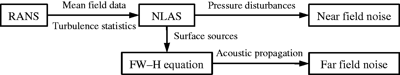
Processes of aerodynamic noise computation.

NLAS method

NLAS method ²³ relies on the concept of disturbances or perturbations computed around a pre-determined mean flow, and uses the priori statistical computations for the sub-grid noise sources. The NLAS method considers a perturbation to the Navier–Stokes equations, in which quantities are split into mean part $\stackrel{-}{\varnothing }$ and fluctuating part $\varnothing \prime$ : $\varnothing =\stackrel{-}{\varnothing }+\varnothing \prime$ . Rearranging fluctuation and mean quantities gives the perturbation equations referred to the nonlinear disturbance equation (NLDE)

$$\frac{\partial {\mathit{Q}}^{\prime }}{\partial t}+\frac{\partial {{\mathit{F}}^{\prime }}_i}{\partial x_i}-\frac{\partial {\left({\mathit{F}}_i^{\nu }\right)}^{\prime }}{\partial x_i}=-\frac{\partial \overline{\mathit{Q}}}{\partial t}-\frac{\partial {\overline{\mathit{F}}}_i}{\partial x_i}+\frac{\partial {\overline{\mathit{F}}}_i{\hspace{0.17em}}^v}{\partial x_i}$$

(1)

$$\overline{\mathit{Q}}=\left[\begin{array}{c}\overline{\rho }\\ \overline{\rho }{\overline{u}}_j\\ \overline{e}\end{array}\right],{\overline{\mathit{F}}}_i=\left[\begin{array}{c}\overline{\rho }{\overline{u}}_i\\ \overline{\rho }{\overline{u}}_i{\overline{u}}_j+\overline{p}{\delta }_{ij}\\ {\overline{u}}_i\left(\overline{e}+\overline{p}\right)\end{array}\right],{\overline{\mathit{F}}}_i^v=\left[\begin{array}{c}0\\ {\overline{\tau }}_{ij}\\ -\overline{\theta }+{\overline{u}}_k{\overline{\tau }}_{ki}\end{array}\right]$$

$${\mathit{Q}}^{\prime }=\left[\begin{array}{c}{\rho }^{\prime }\\ \overline{\rho }{u^{\prime }}_j+{\rho }^{\prime }{\overline{u}}_j+{\rho }^{\prime }{u^{\prime }}_j\\ e^{\prime }\end{array}\right],{\left({\mathit{F}}_i^{\nu }\right)}^{\prime }=\left[\begin{array}{c}0\\ {{\tau }^{\prime }}_{ij}\\ -{\theta }^{\prime }+{u^{\prime }}_k{\overline{\tau }}_{ki}+{\overline{u}}_k{{\tau }^{\prime }}_{ki}\end{array}\right]$$

$${{\mathit{F}}^{\prime }}_i=\left[\begin{array}{c}\overline{\rho }{u^{\prime }}_i+{\rho }^{\prime }{\overline{u}}_i\\ {\rho }^{\prime }{\overline{u}}_i{\overline{u}}_j+\overline{\rho }{\overline{u}}_i{u^{\prime }}_j+\overline{\rho }{u^{\prime }}_i{\overline{u}}_j+p^{\prime }{\delta }_{ij}\\ {u^{\prime }}_i\left(\overline{e}+\overline{p}\right)+{\overline{u}}_i\left(e^{\prime }+p^{\prime }\right)\end{array}\right]+\left[\begin{array}{c}{\rho }^{\prime }{u^{\prime }}_i\\ \overline{\rho }{u^{\prime }}_i{u^{\prime }}_j+{\rho }^{\prime }{u^{\prime }}_i{\overline{u}}_j+{\rho }^{\prime }{\overline{u}}_i{u^{\prime }}_j+{\rho }^{\prime }{u^{\prime }}_i{u^{\prime }}_j\\ {u^{\prime }}_i\left(e^{\prime }+p^{\prime }\right)\end{array}\right]$$

${\tau }^{\prime },\rho \mathrm{\prime }$ , ${u\mathrm{\prime }}_i$ , ${u\mathrm{\prime }}_j$ , ${u\mathrm{\prime }}_k$ , $e^{\mathrm{\prime }},$ and $p\mathrm{\prime }$ are the perturbation time scale, density, velocity components, total energy, and pressure, respectively. ${\delta }_{ij}$ is the kronecker delta. The mean flow quantities are denoted by the superscript “-”. $Q\mathrm{\prime }$ and $\stackrel{-}{Q}$ denote the perturbation variables and transient mean variables, respectively. $F_i\mathrm{\prime }$ is the perturbation inviscid fluxes, comprising both linear and nonlinear terms. ${\stackrel{-}{F}}_i$ represents the mean inviscid fluxes. $\left(F_i^v\right)\mathrm{\prime }$ and ${\stackrel{-}{F}}_i^v$ are the perturbation viscid flux and mean viscid flux, respectively.

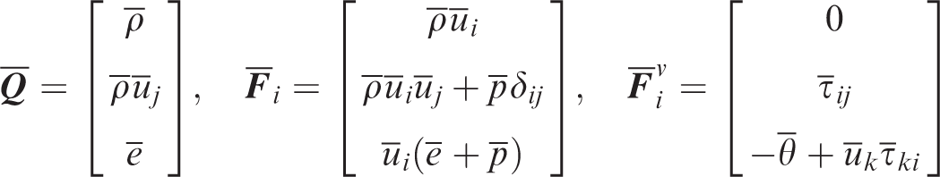
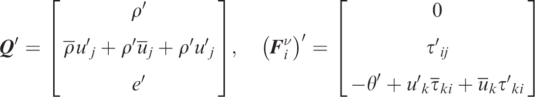
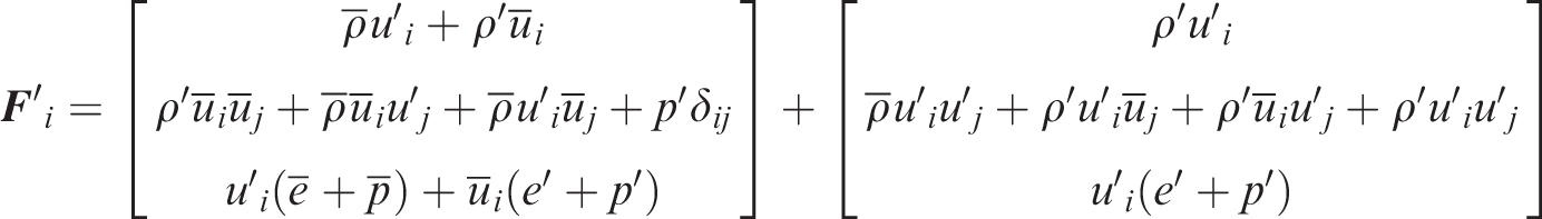
Neglecting density fluctuations and taking time averages of the NLDE cause the linear evolution terms and linear flux terms in the perturbations to vanish. The left and right of the NLDE are represented with $\stackrel{-}{LHS}$ and $\stackrel{-}{RHS}$ respectively, resulting in

$$\overline{\mathit{LHS}}=\overline{\mathit{RHS}}=\frac{\partial {\mathit{R}}_i}{\partial x_i}$$

(2)

in which

$${\mathit{R}}_i=\left[\begin{array}{c}0\\ \overline{\rho }\overline{{u^{\prime }}_i{u^{\prime }}_j}\\ c_p\overline{\rho T^{\prime }{u^{\prime }}_i}+\overline{\rho }\overline{{u^{\prime }}_i{u^{\prime }}_k}{\overline{u}}_k+\frac{1}{2}\overline{\rho }\overline{{u^{\prime }}_k{u^{\prime }}_k{u^{\prime }}_i}+\overline{{u^{\prime }}_k{\tau }_{ki}}\end{array}\right]$$

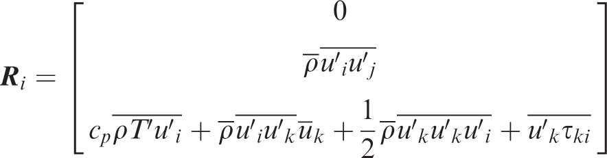
The terms in formula (2) correspond to the standard Reynolds-stress tensor and turbulent heat fluxes. It is essential to obtain these unknown terms from the steady-state RANS simulation in advance. Subsequently, the sub-grid source terms are generated through a synthetic reconstruction of the unresolvable (short wavelength) contribution to the above terms for the NLAS simulation. With both mean levels and sub-grid sources established, time-dependent computations can be implemented to determine the transmitted perturbations using the above set of disturbance equations. NLAS simulation can be achieved in the commercial software now, such as ICFD++.

FW–H acoustic analogy method

The time-dependent surface data computed by NLAS is used to solve the FW–H equation for noise propagations in arbitrary observer points. The penetrable integral solution of FW–H equation solved by Farassat et al.^25–27 can be written in the form of

$$4\pi p^{\prime }\left(x_i,t\right)={{\displaystyle \iint \left[\frac{{\dot{Q}}_j{\hat{n}}_j}{r{|1-M_r|}^2}+\frac{Q_j{\hat{n}}_j\left(r{\dot{M}}_r+c_{\infty }\left(M_r-M^2\right)\right)}{r^2{|1-M_r|}^3}\right]}}_{ret}\text{d}s+{{\displaystyle \iint \left[\frac{L_j{\hat{r}}_j\left(r{\dot{M}}_k{\hat{r}}_k+c_{\infty }\left(M_k{\hat{r}}_k-M^2\right)\right)}{c_{\infty }{r}^2{|1-M_r|}^3}+\frac{L_j{\hat{r}}_j-L_j{M}_j}{r^2{|1-M_r|}^2}\right]}}_{ret}\text{d}s\times {{\displaystyle \iint \left[\frac{{\dot{L}}_j{\hat{r}}_j}{c_{\infty }r{|1-M_r|}^2}+\frac{L_j{\hat{r}}_j-L_j{M}_j}{r^2{|1-M_r|}^2}\right]}}_{ret}\text{d}s+{p^{\prime }}_Q$$

(3)

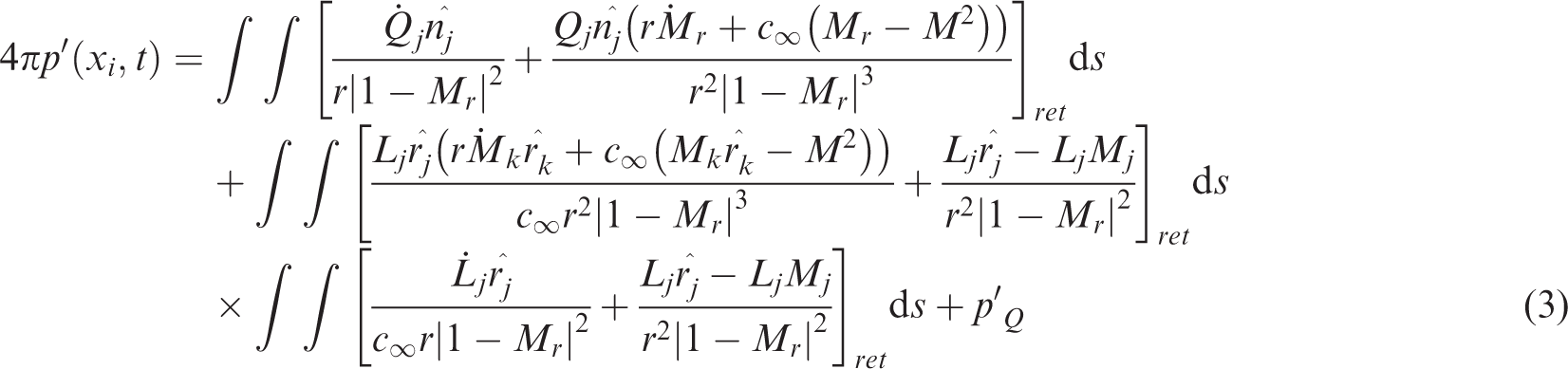
where Q _j = (ρ_∞ − ρ)v_j + ρu_j, L _j = p $\widehat{n}$ _i  + ρu_j (u_i − v_i)n_i, c_∞ and ρ_∞ are the speed of sound and density of undisturbed medium in the far-field; u_i and v_i denote the local velocities of flow medium and body surface respectively; $\widehat{n}$ _i and $\widehat{r}$ _i are the components of unit surface normal vector n and unit radiation vector ( x − y )/r; r = | x − y | is the distance between observer and source positions in which x and y represent observer and source positions, respectively. The symbol [ ] _ret denotes evaluation at the retarded time τ = t − r/c_∞, τ and t are the observer and the source time respectively; M_r = v_i $\widehat{r}$ _i /c_∞ is the Mach number in the observer direction.

Validation of the methodology

Both the surface structure and noise generation mechanism in the windshield region are similar to a simple cavity. To validate the proposed method used in the previous section, two-dimensional simulation is carried out for an aerodynamic noise problem of an open rectangular cavity. As shown in Figure 2, the two-dimensional cavity geometry is taken from the M219 cavity configurations ²⁸ with a length-to-depth (L/D) ratio of 5. Its depth D is equal to 101.6 mm. The total length of the computational domain in the x-axis (streamwise) is 11D from x/D=−2 to 9 and in the y axis (wall-normal) is 6D from y/D=−1 to 3. The whole cavity model consists of about 35,000 cell volumes (CVs) with 16,800 CVs inside the cavity. The cell size of boundary layer meshes on the cavity wall starts at 0.004D and expands exponentially along the wall normal direction. The flow conditions correspond to a free-stream Mach number of 0.85 and a Reynolds number of 6.8 million based on the cavity length. The stagnation pressure and temperature are set to 99,600 Pa and 305 K, respectively. In order to obtain the oscillation pressure and noise signal in the cavity, ten measuring points named K20 to K29 are arranged on the cavity ceiling from x/L = 0.05 to 0.95 with increment of 0.5D. Finally, the NLAS transient simulation is carried out with a physical time step of 2 × 10⁻⁵ s.

Figure 2.

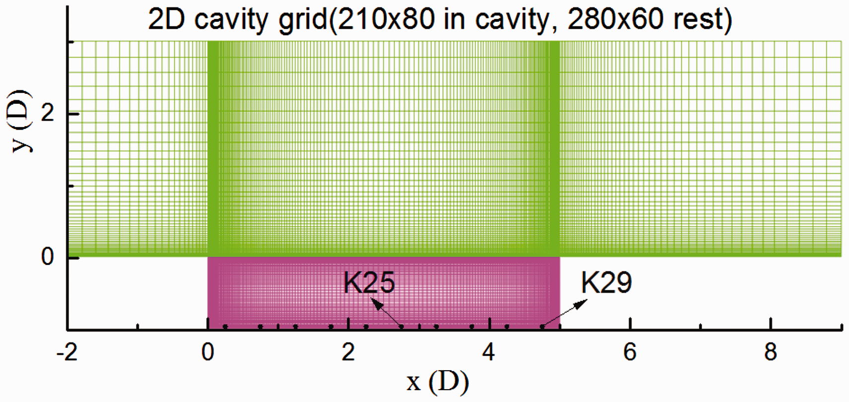
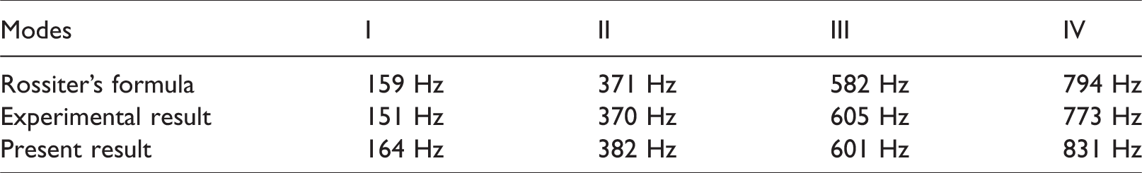
A schematic of 2D cavity grid, unit in D.

When the pressure fluctuations captured at measuring points occur periodically, the following pressure signals are kept until 0.2 s. The periodical pressure fluctuations indicate that pressure oscillations are already full developed and continued. Then, pressure signals are processed through fast Fourier transform with a sampling rate of 6k Hz in accordance with the experimental one. The computational sound pressure level (SPL) spectrums at the K25 and K29 positions are shown in Figure 3. Since the low-frequency components of computed SPL spectrums are related to resonances inside the cavity, SPL peaks occur at the corresponding mode frequencies. Four SPL peaks are obviously captured below 1k Hz in Figure 3(b) and the corresponding frequencies are the first four-order mode frequencies, which are 164 Hz, 382 Hz, 601 Hz, and 831 Hz, respectively. The comparisons of mode frequencies at K29 between experimental data ²⁸ and prediction by Rossiter’s formula ²⁹ are listed in Table 1. The calculated mode frequencies are slightly larger than the experimental values with relatively errors of 8.6%, 3.2%, 0.7%, and 7.5%. In addition, the computed mode frequencies agree better with Rossiter’s semi-empirical predictions with the errors of 3.1%, 3.0%, 3.3%, and 4.7%, respectively. Consequently, the mode frequencies are well predicted with respect to the experimental data and Rossiter’s formula. In addition, the comparisons of SPL spectrums at K25 and K29 are also shown in Figure 3. The mode amplitudes are well predicted with the errors of no more than 5 dB. And computational SPL spectrums are also in good agreement with the experiment ones. Besides, the overall or band-limited root-mean-square (RMS) pressure distributions are calculated along the cavity ceiling and compared with the experimental and other numerical results in Figure 4. The RMS pressure is slightly over predicted with smaller discrepancy compared with LES and DES results.^30,31 Therefore, the accuracy of the proposed hybrid computational methodology has been validated.

Figure 3.

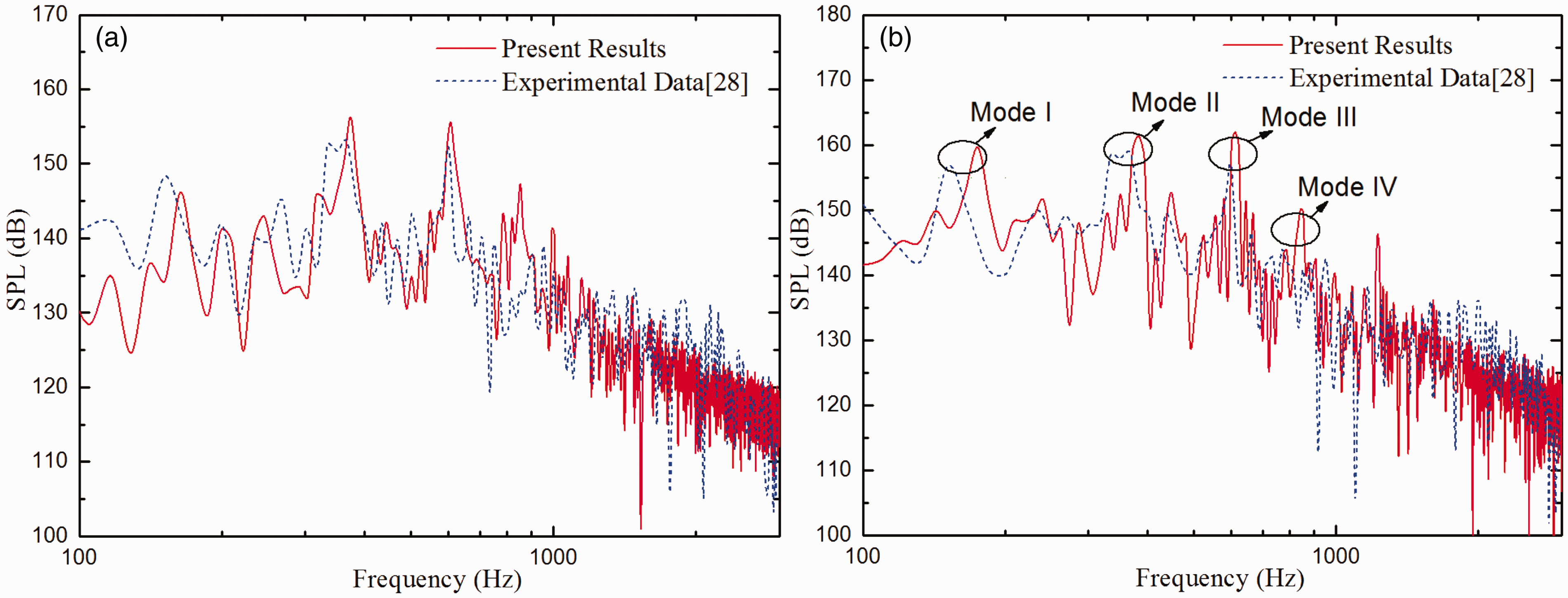
Comparisons of SPL spectrum: (a) K25 position, (a) K29 position.

Table 1.

Comparisons of mode frequencies at K29.

Modes	I	II	III	IV
Rossiter’s formula	159 Hz	371 Hz	582 Hz	794 Hz
Experimental result	151 Hz	370 Hz	605 Hz	773 Hz
Present result	164 Hz	382 Hz	601 Hz	831 Hz

Figure 4.

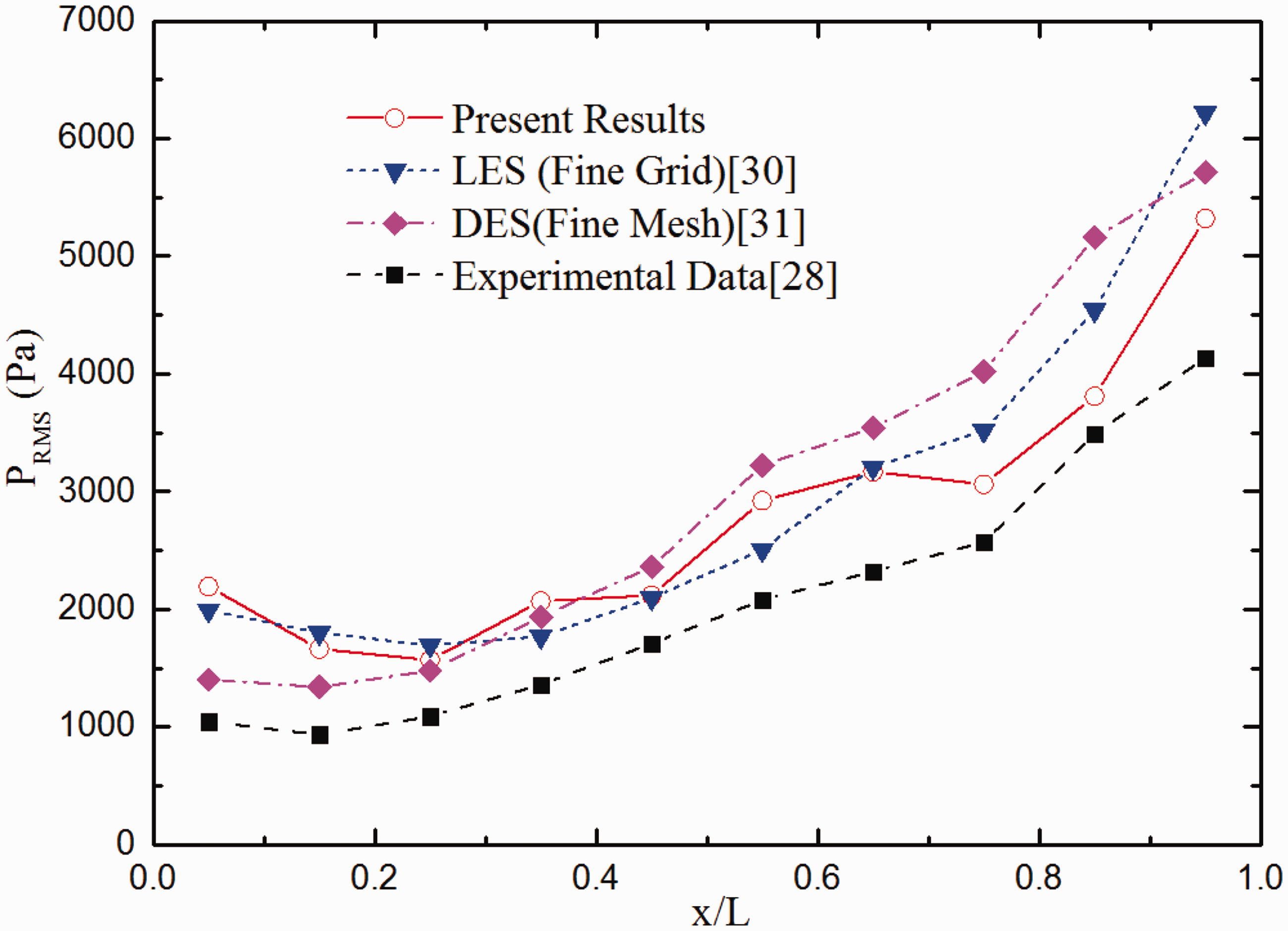
Comparisons of RMS pressure along the cavity ceiling.

Computational configurations

Model description

The windshield region model in this paper is obtained from Chinese CRH series high-speed train with an inter-coach gap of 0.85 m, as shown in Figure 5. The simplified train model consists of a head coach and a tail coach, ignoring the bogie and pantograph systems, but retaining the air-conditioning cover characteristics around the windshield area and wrinkle characteristics on windshield surfaces. The train model size is about L = 51.5 m, W = 3.2 m, and H = 3.6 m. Figure 6 shows a schematic diagram of the computational domain. The dimensions of the computational domain are 3L (streamwise) $\times$ 5W (spanwise) $\times$ 5H (ground-normal). The train model is placed at the central position both in the streamwise and spanwise direction, and with a distance of 0.325 m from the ground. As we focus on the noise problem in the windshield area, the boundary effects in the streamwise direction can be ignored. Meanwhile, the boundaries are far enough in the spanwise direction and ground normal direction, which means the outside boundary effects of the computational domain on the flow field in the windshield area can also be ignored.

Figure 5.

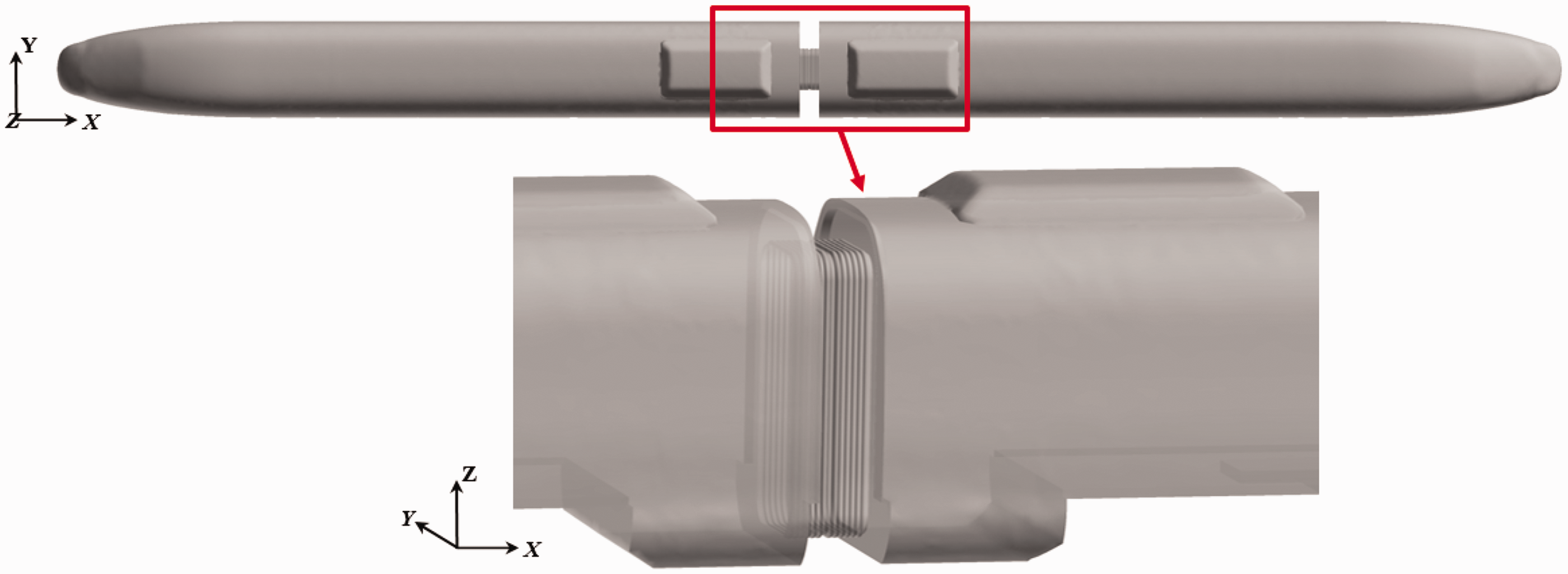
Computational models of the train and inter-coach windshield region.

Figure 6.

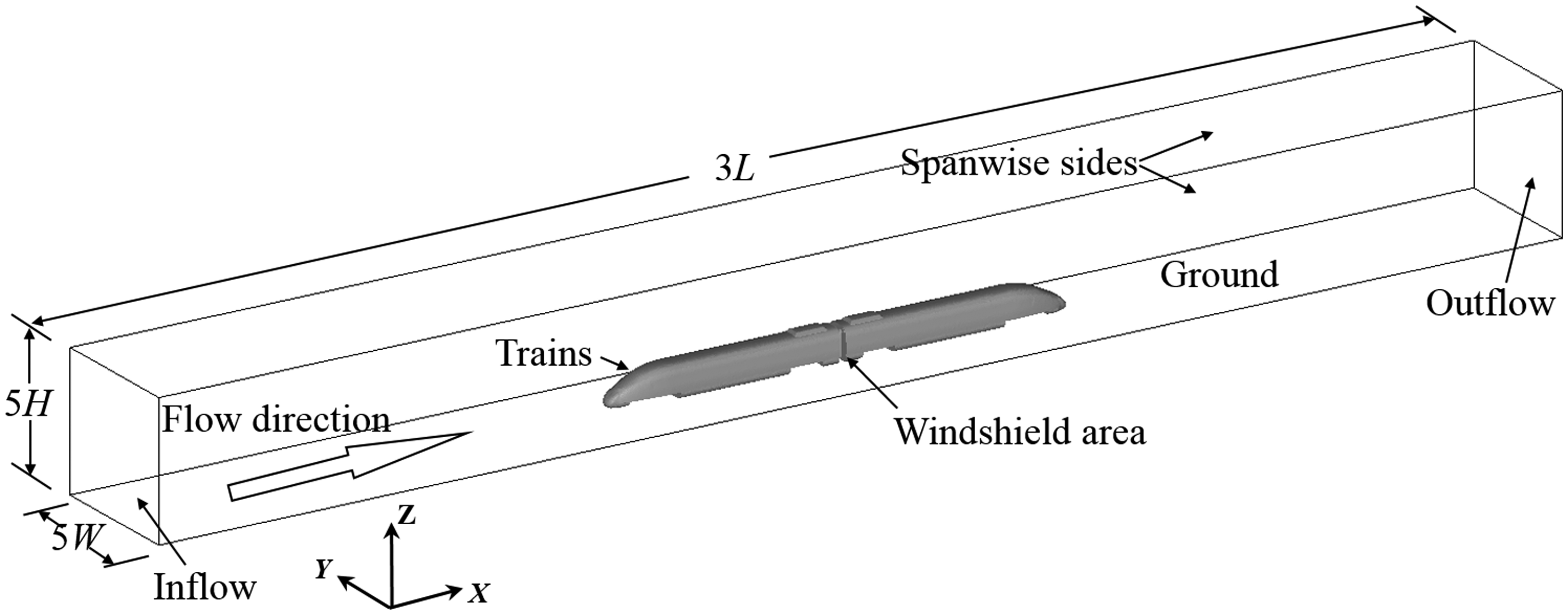
Schematic diagram of the computational domain.

The computational domain is discretized by a hybrid grid strategy with a total cell volume of about 9.5 million, as partially shown in Figure 7. Hexahedrons are adopted in the far-wall region, while tetrahedrons are used in the near-wall region, and the two parts are connected together with pyramids. The grids around the windshield area are refined to capture more details of flow field and noise characteristics. The size of surface meshes around the windshield region is not larger than 15 mm, while the grid size of flow field in the windshield region is less than 50 mm. In order to consider the near-field boundary layer effect more appropriately, 15 layers of triangular prisms are created on surfaces in the windshield region.

Figure 7.

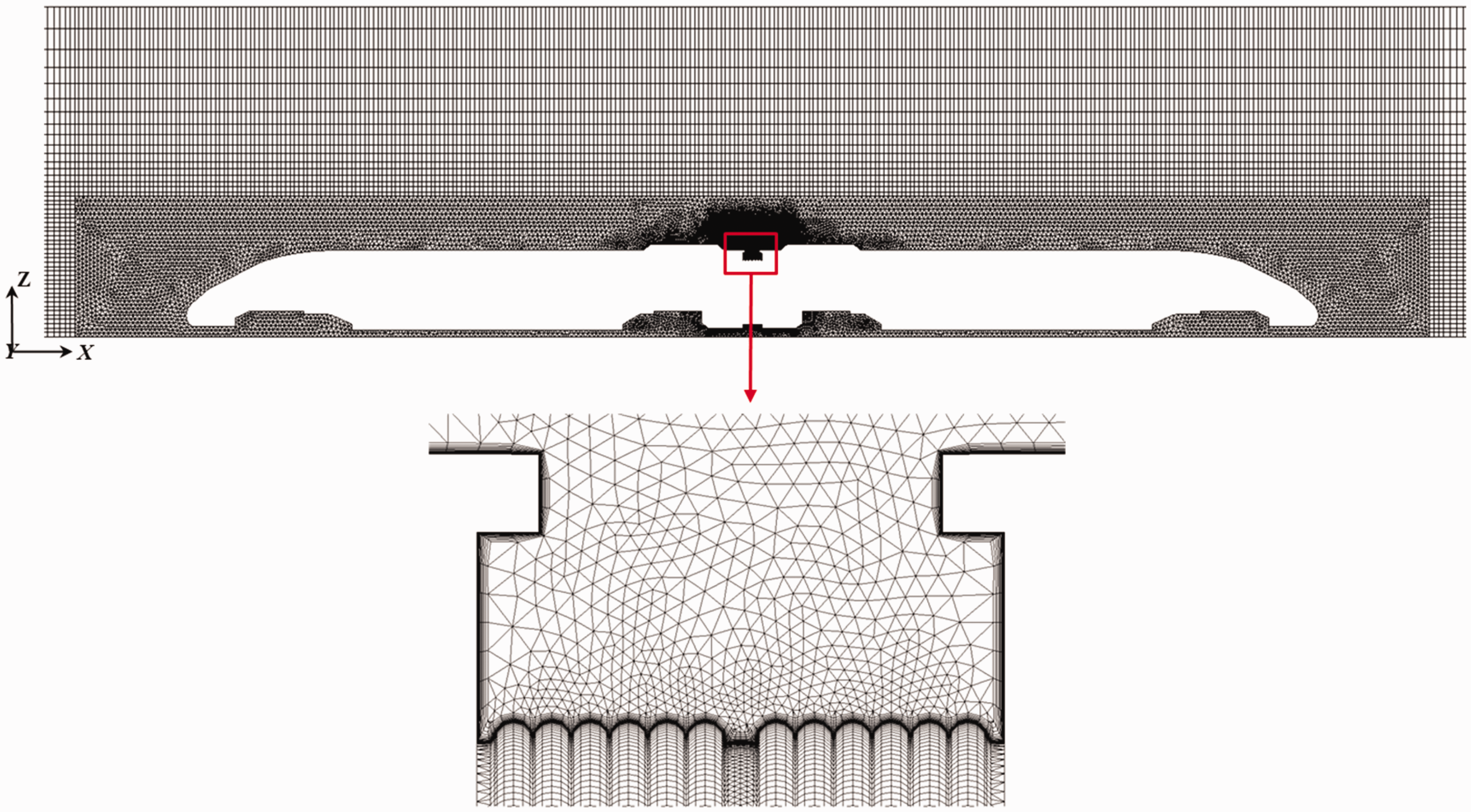
Schematic diagram of grid distribution around the train model and inter-coach windshield region.

Computational conditions

The incoming flow condition corresponds to the free-stream velocity of 350 km/h. The static pressure and temperature are set to 0.1 MPa and 298.15 K. The free-stream viscosity is assumed to change with the temperature in Sutherland’s law. During the steady RANS computation, the train is assumed to be stationary, and the nonslip wall condition is adopted for the solid surfaces. The ground of the wind tunnel model is set as moving wall at the same speed of incoming velocity and the other tunnel boundaries are characteristic boundary conditions corresponding to the free-stream velocity. During the NLAS transient calculation for aerodynamic noise simulation, the wall conditions of solid surfaces and the ground remain the same, while the rest walls adopt NLAS outer boundary conditions. To prevent the acoustic field being polluted by the sound waves reflection at the outer boundaries, three absorption layers are set on these outer boundaries.

A total of 2000 steps are calculated and the steady RANS calculation achieves a sufficient convergence. The time-step size in the NLAS transient calculation is set to 20 μs, and the maximum analysis frequency of aerodynamic noise results is 25k Hz accordingly. About 10,000 steps are applied for the simulation with total physical time of 0.2 s in the transient simulation.

Results and discussions

Flow field results

Turbulent intensity

Figure 8 shows a snapshot of the intensity of turbulent kinetic energy distribution around the train on the central plane. It is noticed that the large turbulent intensity of flow field is distributed in the bogie region, the windshield region, and the tail vortex region. Especially in the windshield region, high intensity turbulence energy appears inside the cavity and behind the air-conditioner covers owing to serious irregularities of the coach body surfaces. Therefore, these areas are supposed to be important aerodynamic noise sources.

Figure 8.

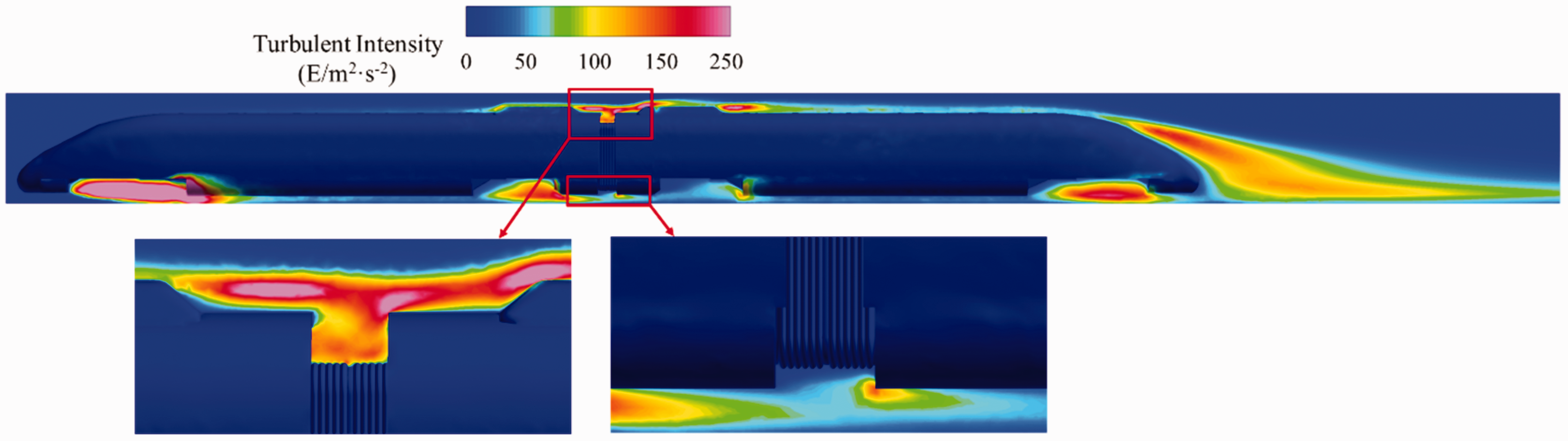
Snapshot of the intensity of turbulent kinetic energy on the central plane of computation domain.

Surface fluctuating pressure and wall shear stress

According to the aerodynamic noise theory, surface fluctuating pressure and wall shear stress are the main causes of dipole sound sources. Figure 9 shows instantaneous contours of surface fluctuating pressure and wall shear stress on the coach surface in the windshield region. The results indicate that the surface fluctuating pressure and wall shear stress are mainly distributed on the downstream surface around windshield region. And they are much larger on the surfaces at the top of windshield area than that at the other positions, such as both sides and the bottom. Furthermore, the orders of magnitude of surface fluctuating pressure and wall shear stress have been analyzed as a result of 10⁴ and 10¹ respectively, indicating that the fluctuating pressure is the main cause of the dipole noise source in the windshield region.

Figure 9.

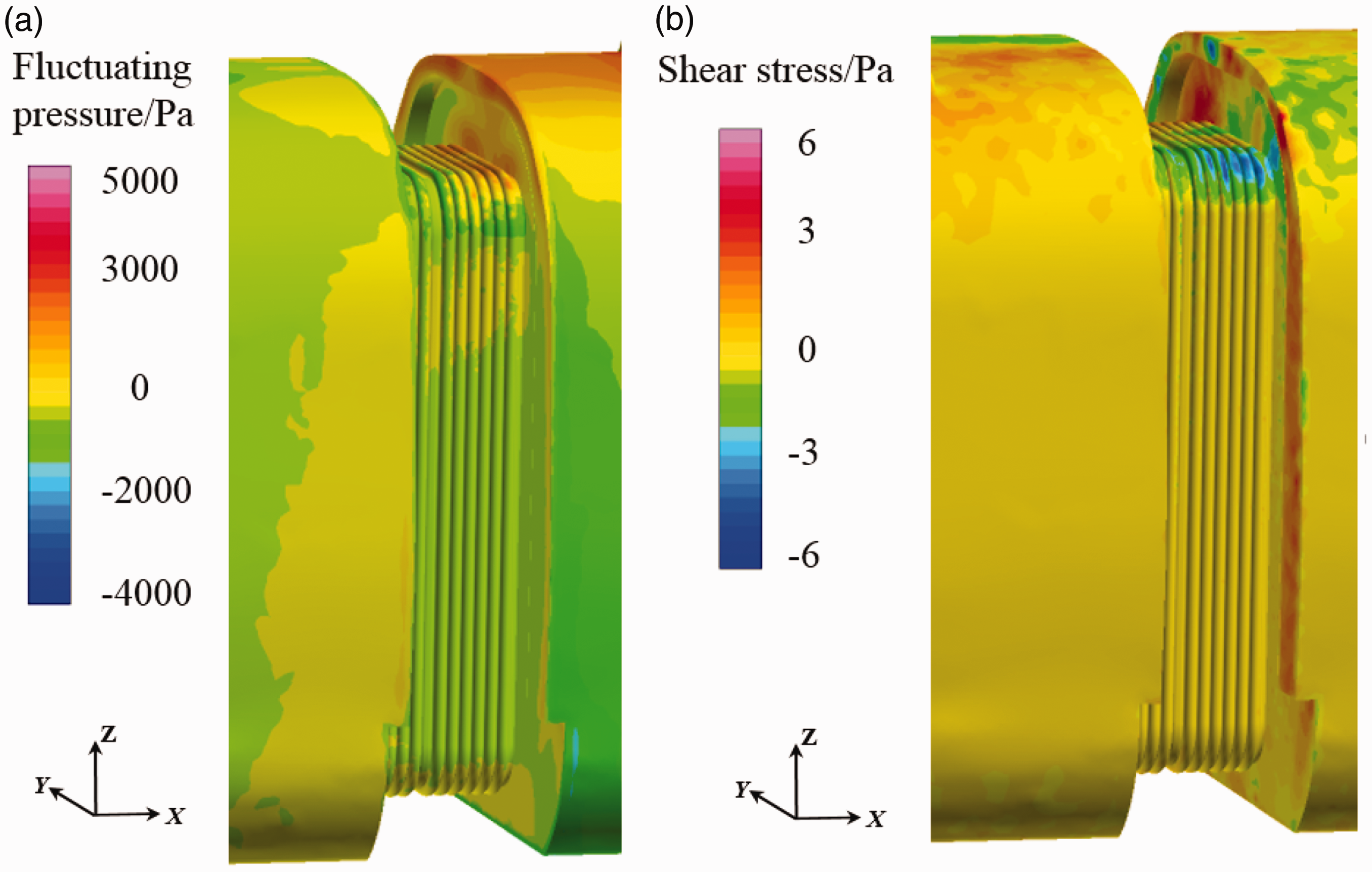
Instantaneous contours of flow variables on the surfaces in windshield region: (a) surface fluctuating pressure, (b) wall shear stress.

Contours of vortices

Figure 10 shows the instantaneous contours of vortices on the different planes. The contours of vortices on the Z–X planes in Figure 10(a) and (b) indicate that lots of vortices are located in the position close to the carriage surfaces on both sides of windshield region, while the vortices are mainly at the top of the cavity on both sides. There are more and smaller vortices at the top of the windshield region than that at the bottom in Figure 10(c), indicating that airflow disturbance at the top is more intense. This phenomenon is the consequence of higher bench height and installation of air-container covers at the top. As shown in contours of vortices on the Y–X planes and Z–Y planes in Figure 10(d) to (f), the vortices shedding from the upstream strike upon the downstream edge of the inter-coach and form strong feedback flow to fill the entire cavity. Besides, in Figure 10(d) to (e), there are very intense vortices around Z-axis inside both sides of the cavity. As shown by the streamlines in Figure 10(g), strong spiral flow around Y-axis is generated at the top of the cavity, and spirals downward with another two spiral flow around Z-axis since both sides of the cavity are open areas. Complex three-dimensional effect exists in the inter-coach windshield region, where is full of vortex around different axes. Consequently, the feedback and inside oscillation of the cavity flow will generate aerodynamic noise sources with high energy.

Figure 10.

Instantaneous contours of vortices on the different planes and flow streamlines: (a) Y=−1.5 m, (b) Y=−0.8 m, (c) Y = 0 m, (d) Z = 2 m, (e) Z = 3.6 m, (f) X = 0 m, (g) flow streamlines.

Near-acoustic field

Near-field noise characteristics

A series of measuring points are arranged in the near-field area around the windshield to obtain near-field noise results, as shown in Figure 11. A total of 14 measuring points are arranged on two planes perpendicular to the streamwise direction, where P1–P7 are on the upstream plane and P8–P14 are on the downstream plane. All the points are distributed at the top, one side, and the bottom of the windshield region, respectively.

Figure 11.

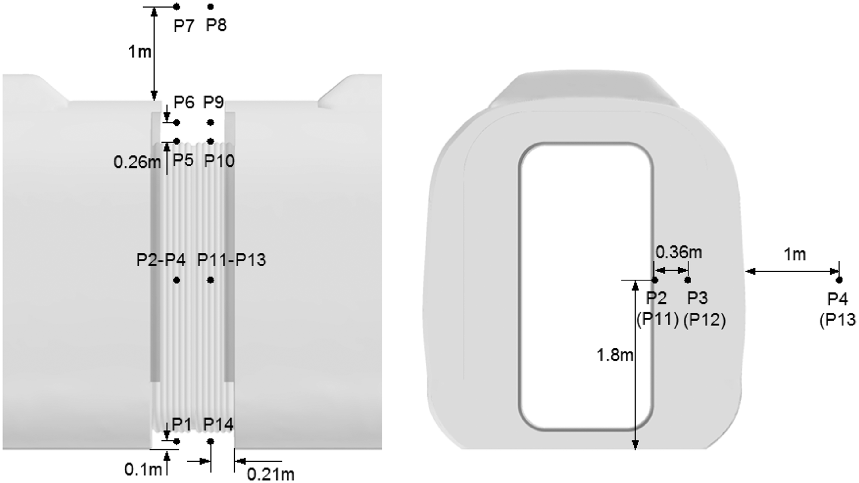
Near-field measuring points around the windshield region.

The time domain sound pressure results are obtained from the measuring points, and fast Fourier transform needs to be applied to obtain the sound pressure spectrum. The amplitude of noise is expressed in terms of sound pressure level (SPL) in the unit of decibel (dB), defined as

$$L_p=20\lg \frac{p_e}{p_{ref}}$$

(4)

where p_e represents the effective sound pressure corresponding to the root mean square of the instantaneous sound pressure; p_ref is the reference sound pressure, which is the value that can be perceived by human ears with the frequency of 1k Hz, p_ref =20 μPa. In addition, the overall sound pressure level (OASPL) of observer points can be calculated by summing up all the acoustic energy over the entire frequency domain, expressed as

$$L_{pz}=10\lg {\displaystyle \sum _i{10}^{L_{pi}/10}}$$

(5)

The narrow-band SPL frequency spectrums of the aerodynamic noise at P9–P12 inside the cavity are shown in Figure 12. The frequency interval is 2.5 Hz and the frequency range is from 10 Hz to 5k Hz. It can be obviously demonstrated by the frequency spectrums that most of the acoustic power is concentrated in the low-middle frequency range below 500 Hz and the SPL peaks appear at the frequency of 41.2 Hz, 36.1 Hz, 42.5 Hz, and 42.1 Hz respectively at P9–P12. As described above, the flow in the windshield region is a typical cavity flow. The acoustic energy within the low-frequency range (below 100Hz) closely corresponds to the self-excited resonance of the flow inside the cavity, and the mode frequency of the cavity in the windshield region can be calculated by Rossiter’s-empirical formula ²⁹

$$f_n=\frac{U_{\infty }\left(n-\gamma \right)}{L\left(M_{\infty }/\sqrt{1+\left(\gamma -1\right)M_{\infty }^2/2}+1/\kappa \right)}$$

(6)

where U_∞ and M_∞ are the free-stream velocity and Mach number, respectively. L is the length of the cavity and n is the mode number. κ  =  0.57 and γ  =  0.25 are empirical constants. The first-order mode frequency is predicted to be 42 Hz, which is closed to the calculated frequency of the SPL peak and demonstrates the effectiveness of the calculations. Besides, aerodynamic noise inside the cavity is typical broadband noise in the frequency range from 100 Hz to 5k Hz or above without specific peaks.

Figure 12.

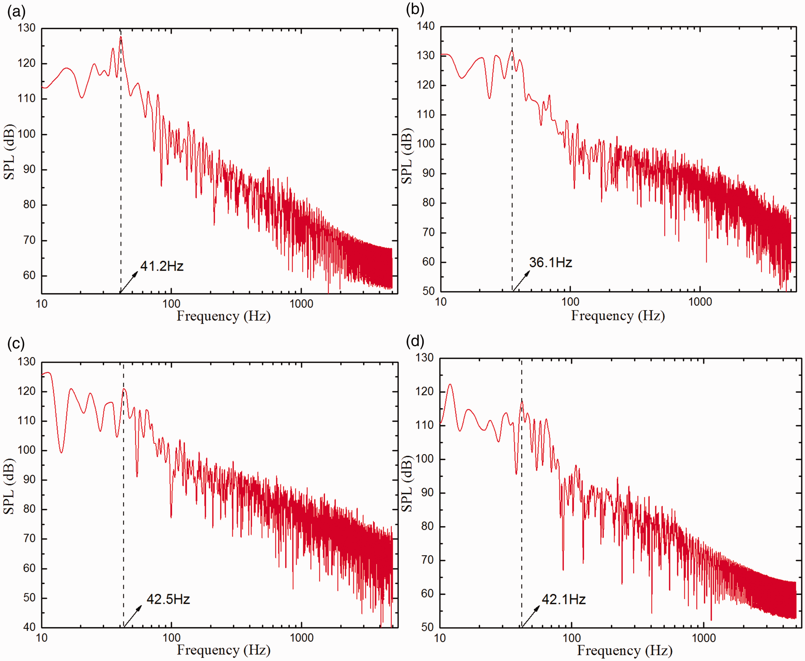
Computational SPL frequency spectrum of measuring points insides the cavity: (a) P9, (b) P10, (c) P11, (d) P12.

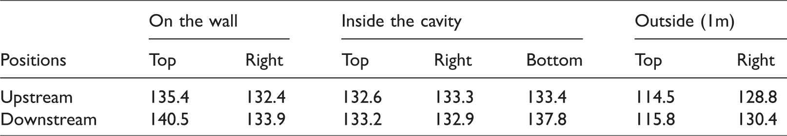
The OASPLs at measuring points are shown in Table 2, and aerodynamic noise around the windshield is seriously noisy. Aerodynamic noise at the downstream position of the cavity is larger than that at the upstream position due to the upstream swirl flow directly impacting on the downstream surfaces. Aerodynamic noise at the top is loudest corresponding to the flow field results because the air-conditioner covers enhance the turbulent intensity. Moreover, the spiral flow is formed at the top and develops downward to fill the both open sides with basically the same turbulent intensity. As a result, the OASPL at different points inside the cavity maintains at a same level of about 133 dB, and the OASPL at the bottom is higher due to the strong turbulence generated by the upstream bogie area.

Table 2.

Computational OASPL at measuring points (dB).

Positions	On the wall		Inside the cavity			Outside (1m)
	Top	Right	Top	Right	Bottom	Top	Right
Upstream	135.4	132.4	132.6	133.3	133.4	114.5	128.8
Downstream	140.5	133.9	133.2	132.9	137.8	115.8	130.4

Acoustic pressure distribution

Near-field acoustic pressure results can be obtained directly after NLAS transient calculations. Figure 13 shows the acoustic pressure distribution around the train on the Y–X plane (Z = 2 m) and Z–X plane (Y=−0.1 m). The red and blue colors indicate the positive and negative sound pressure regions.

Figure 13.

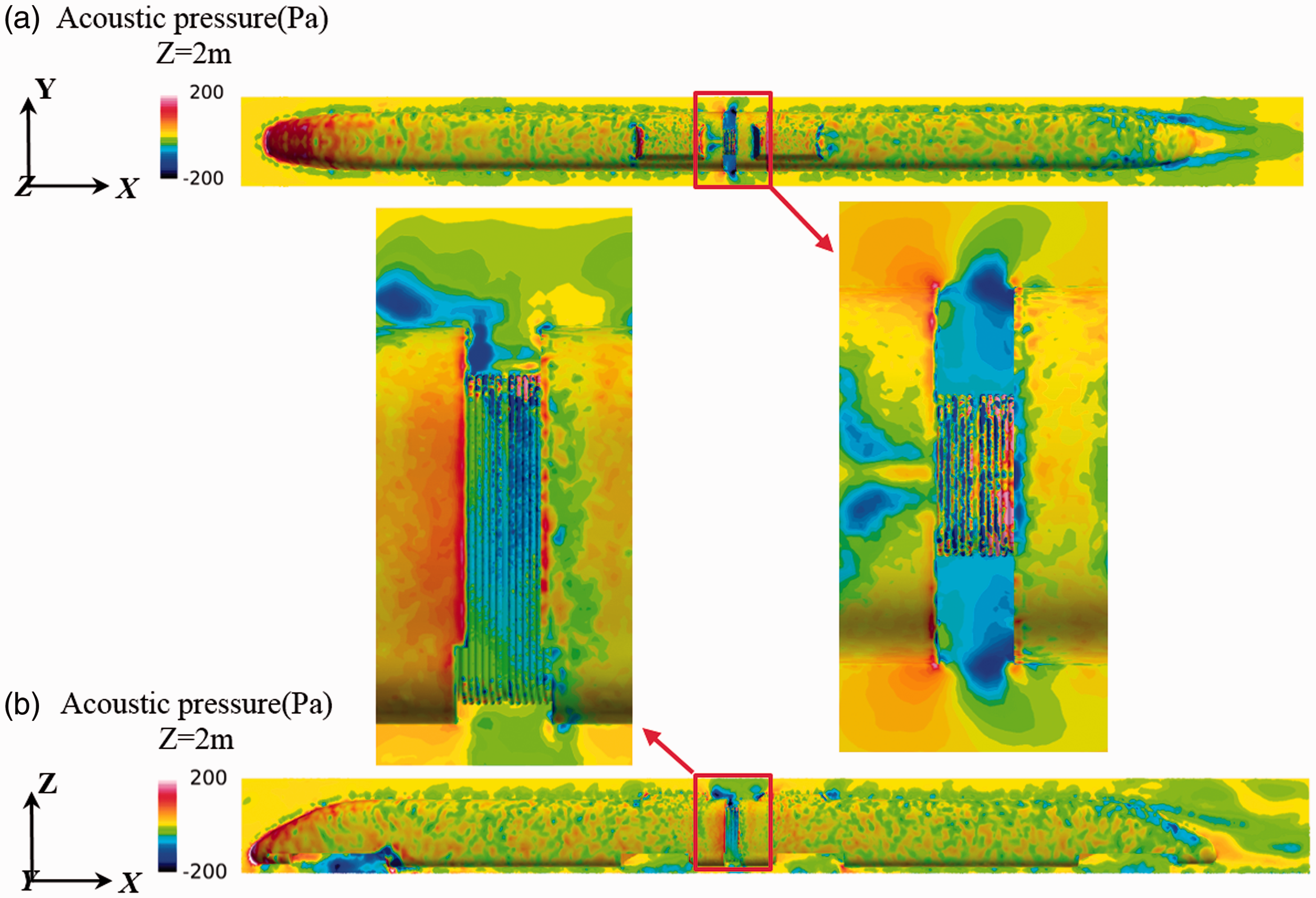
Acoustic pressure distribution around the train: (a) Z = 2 m, (b) Y=−0.1 m.

As shown in Figure 13, the locations of a larger absolute value of the acoustic pressure are concentrated in the regions around uneven train coach surfaces such as the head, the windshield area, the bogie area and the tail area, which corresponds to the distribution of turbulent kinetic energy. The details in the windshield region show the absolute values of acoustic pressure on the coach body surfaces of the windshield region are rather large, indicating that the energy of the dipole noise sources around surfaces is pretty high. At the top of the windshield, the acoustic pressure on the downstream surfaces is mainly positive, while on the upstream surfaces it is mainly negative. The main reason for the distribution is upstream vortices at the top strike on the downstream surfaces directly, which will generate a strong backflow and scour the upstream surfaces. In addition, due to the strong swirling flow generated inside the cavity and behind the air-conditioner cover, the acoustic pressure inside the cavity and at the top is mostly negative.

It is also noticed that there are two-lobe shapes of acoustic pressure distribution on both sides in the windshield area. And one lobe is positive and pointing upstream while the other is negative and pointing downstream, and the dividing point of the two-lobe shape is at the upstream edge of the train coach. The formation of the two-lobe could be the consequence of the vortices shedding from the upstream edge along the streamwise direction and the inside flow self-excited oscillations. Besides, the upstream vortex collides with the downstream edge of the cavity, which generates the irregular flow on the downstream coach surface. The surface pressure changes rapidly, which is also enhanced by the downstream air-conditioner covers. As a result, the downstream coach surfaces also become an important noise sources.

Longitudinal distribution of near-field noise

In order to obtain the distribution of near-field noise in the velocity direction, a series of measuring points are arranged at the distance of 1 m from the coach surface and 3.5 m from the ground with the intervals of 1 m or 5 m around the windshield, the head and tail respectively.

The measuring points and corresponding OASPL along the free-stream are shown in Figure 14. The results indicate the OASPL of the aerodynamic noise is remarkable around the front, windshield area, and tail area, also corresponding to the turbulence intensity distribution mentioned above. Two significant peaks can be clearly captured at the position of 3 m away from the windshield upstream and downstream respectively, while around the windshield that is a trough on the contrary. The two lobes of the acoustic pressure distribution on the sides of the windshield area can be considered as two sound sources pointing to upstream and downstream respectively. Therefore, the noise facing the windshield may be weakened by the two sound sources interference, while that at the both sides may also be enhanced by the interference, corresponding to the OASPL troughs and peaks. Besides, the peak positions are near the bogie area and air-conditioner covers corresponding to high turbulent intensity. As a result, the factors described above possibly have effects on the appearance of OASPL peaks on the sides.

Figure 14.

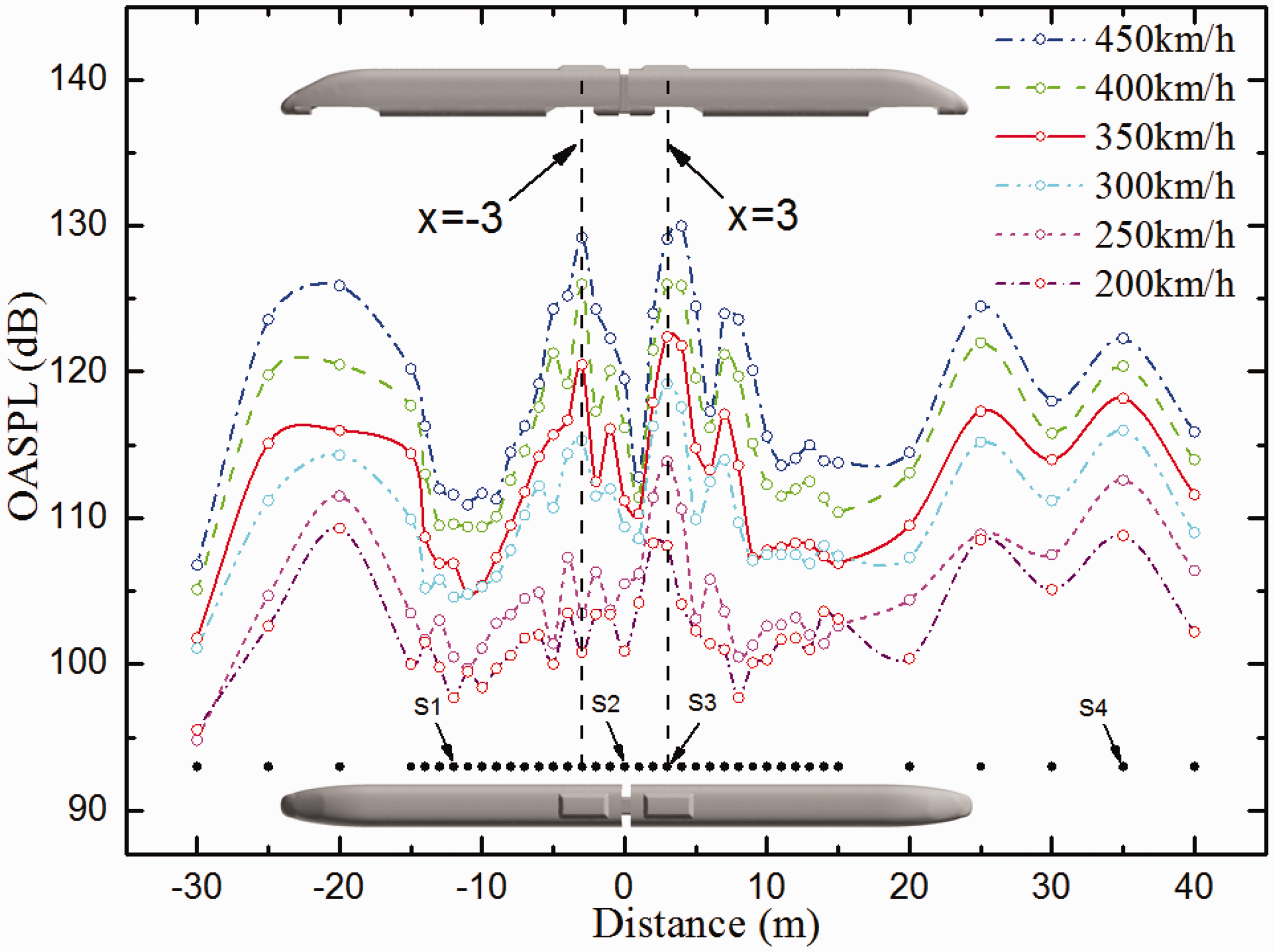
The longitudinal distribution of near-field noise around the train at different speed levels.

In addition, Figure 14 also shows the distribution of OASPL along the streamwise direction at different speed levels, indicating that the OASPL increases remarkably with the speed.

Near-field noise with respect to different speed levels

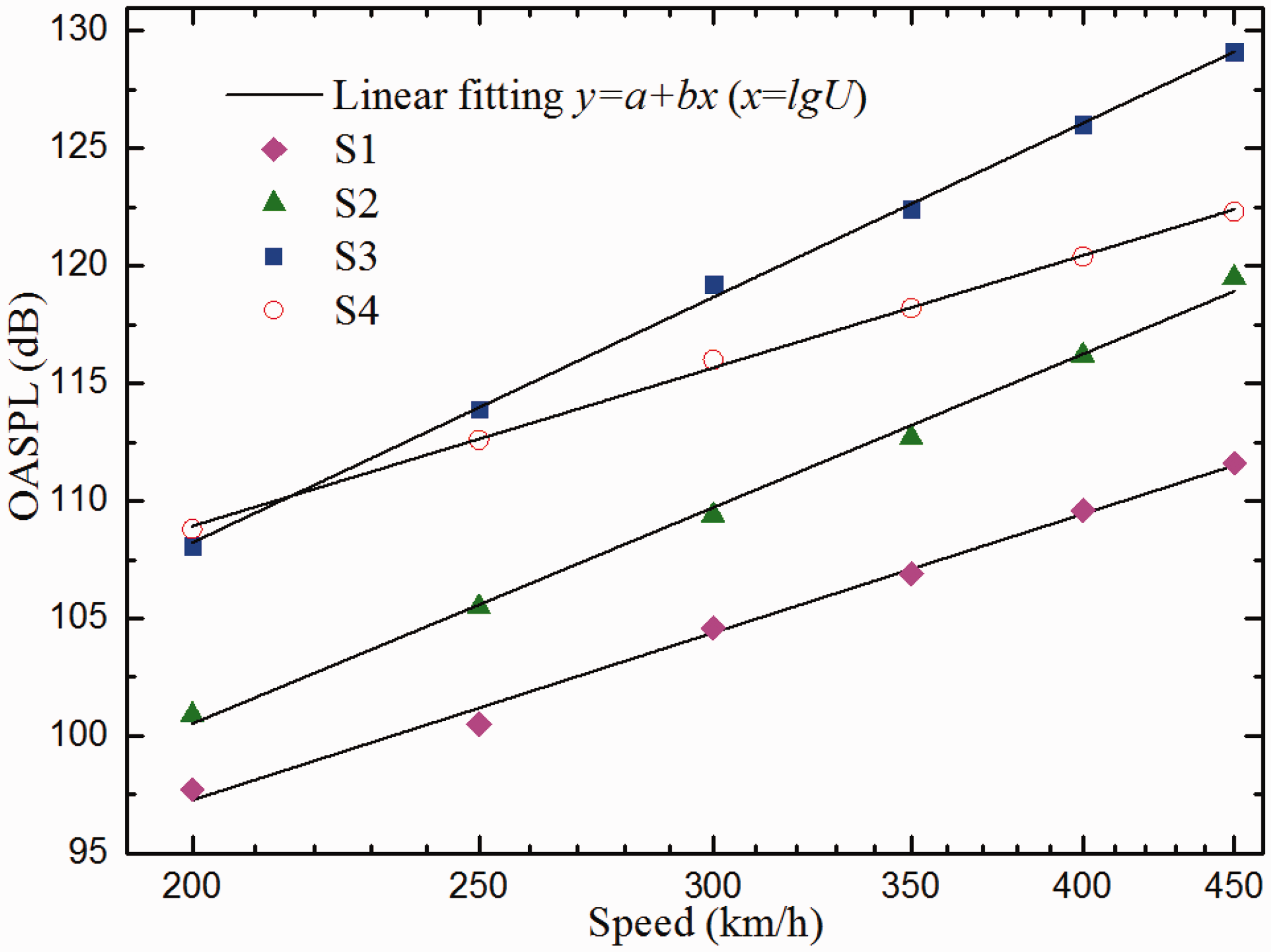
The previous studies have shown that the aerodynamic noise around the train is closely related to the speed levels. In this section, the variation of the aerodynamic noise in the windshield region with train speed will be further discussed. Several measuring points are chosen from Figure 14 and named as S1–S4, corresponding to the location where coach surfaces are smooth (x=−12 m), the position where is apposite the windshield (x = 0 m), the position where the OASPL peak appears (x = 3 m) and the position where is at the wake flow (x = 35 m), respectively. The variations of OASPL versus train speed at different points are displayed in Figure 15. The points of different symbols represent the calculated values while the solid lines are logarithm-fitting curves of the data, which can be written in the form of the equation as

$$L_{pZ}=a\lg \left(U/U_0\right)+L_{pZ0}$$

(7)

where L_pZ0 is the OASPL at the speed of U₀ and a is the slope value, and a = 52.26 at S2 point. Since the definition of SPL can be written as another form, $L_p=10\mathrm{l}\mathrm{g}(p_e^2/p_{ref}^2)$ , the square of effective sound pressure $p_e^2$ can be considered as a form of energy, which indicates that the SPL also represents a ratio of a certain energy and reference energy. Therefore, compared with the definition formula of SPL, the acoustic power of aerodynamic noise radiated from the windshield region (S2) is approximately proportional to the 5th power of train speed. By the same method, the variation of OASPL versus speed can be obtained at S1, S3, S4 points. The slope values of the fitting curves a are 40.45, 59.31, and 38.26 respectively, and the aerodynamic noise at S1, S3, and S4 approximately grows as power law of speed to the order of 4th, 6th, and 4th, respectively.

Figure 15.

Variations of OASPL versus speed at measuring points.

Far acoustic field

In order to obtain far-field noise results, it is necessary to capture and store the noise sources around computational model during NLAS transient calculation. The rectangular meshes are created surrounding the train model, which is longer owing to the complex flow in the tail area. Five surfaces are taken as integral control surfaces for the far-field noise propagation except the ground surface due to the ground effect. Aerodynamic noise at far-field measuring points can be obtained through the integrals of FW–H formulation over the pre-arranged integral surfaces.

Noise characteristics at far-field measuring points

Far-field noise is an important index to evaluate the noise of high-speed train. According to the international standard ISO3095-2005, the sampling data would be gathered at the standard observation point which is 25 m away from the centerline of rail track and 3.5 m above the surface of rail track. In this study, the standard measuring point is set opposite the windshield with coordinates of (0 m, 25 m, 3.5 m). The SPL is used to evaluate the noise level according to the standard.

Figure 16 shows the one-third octave band frequency spectrum of aerodynamic noise at the speed of 350 km/h at the standard observation point, with frequency range from 10 Hz to 5k Hz. The aerodynamic at the far-field standard observation point is mainly concentrated on the low-middle frequency range below 500 Hz.

Figure 16.

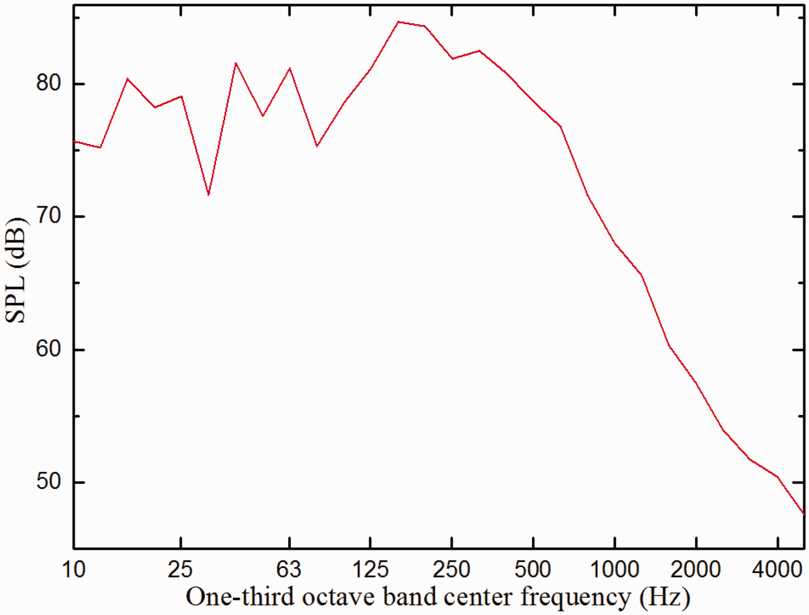
One-third octave band frequency spectrum of aerodynamic noise at the standard observation point.

Acoustic attenuation with respect to distance

In order to explore the near-field noise attenuation with the distance, six measuring points are arranged horizontally around the windshield region and the distance from the centerline is 2.6 m, 6.25 m, 12.5 m, 25 m, 50 m, 100 m, and 200 m, respectively. The coordinates of the measuring points are shown in Table 3.

Table 3.

Coordinates of measuring points.

Observation sites	1	2	3	4	5	6	7
X-coordinate (m)	0	0	0	0	0	0	0
Y-coordinate (m)	2.6	6.25	12.5	25	50	100	200
Z-coordinate (m)	3.5	3.5	3.5	3.5	3.5	3.5	3.5

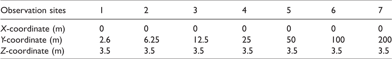
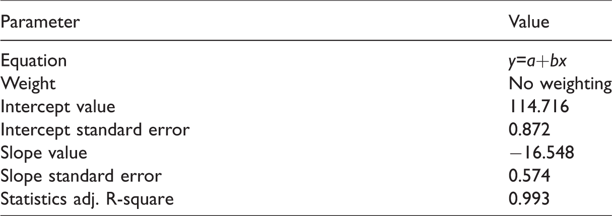
Figure 17 shows the attenuation of the OASPL with the distance at measuring points, where the solid box points are calculated values and the solid line is the corresponding logarithm-fitting curve. The fitting parameters in Figure 17 are listed in Table 4 and the slope value is −16.55 in the logarithmic coordinate, which means acoustic attenuation is 16.55lg2 = 4.98 dB with the distance doubled. As is known, the SPL of the spherical wave is attenuated by 6 dB with twice the distance, while the attenuation value of the cylindrical wave is 3 dB. The result implies that the near-field aerodynamic noise radiated from the windshield region propagates outward unlike a point sound source or a line sound source. The reason is that the near-field aerodynamic noise on both sides in the windshield region can approximately be considered as two line sources distributed on the upstream and downstream edges of the coach respectively, as mentioned above. In contrast, the magnitude of acoustic attenuation is about 6 dB when the observation site is far from 50 m, implying that the aerodynamic noise radiates outward primarily in the form of the spherical wave as farther than 50 m away.

Figure 17.

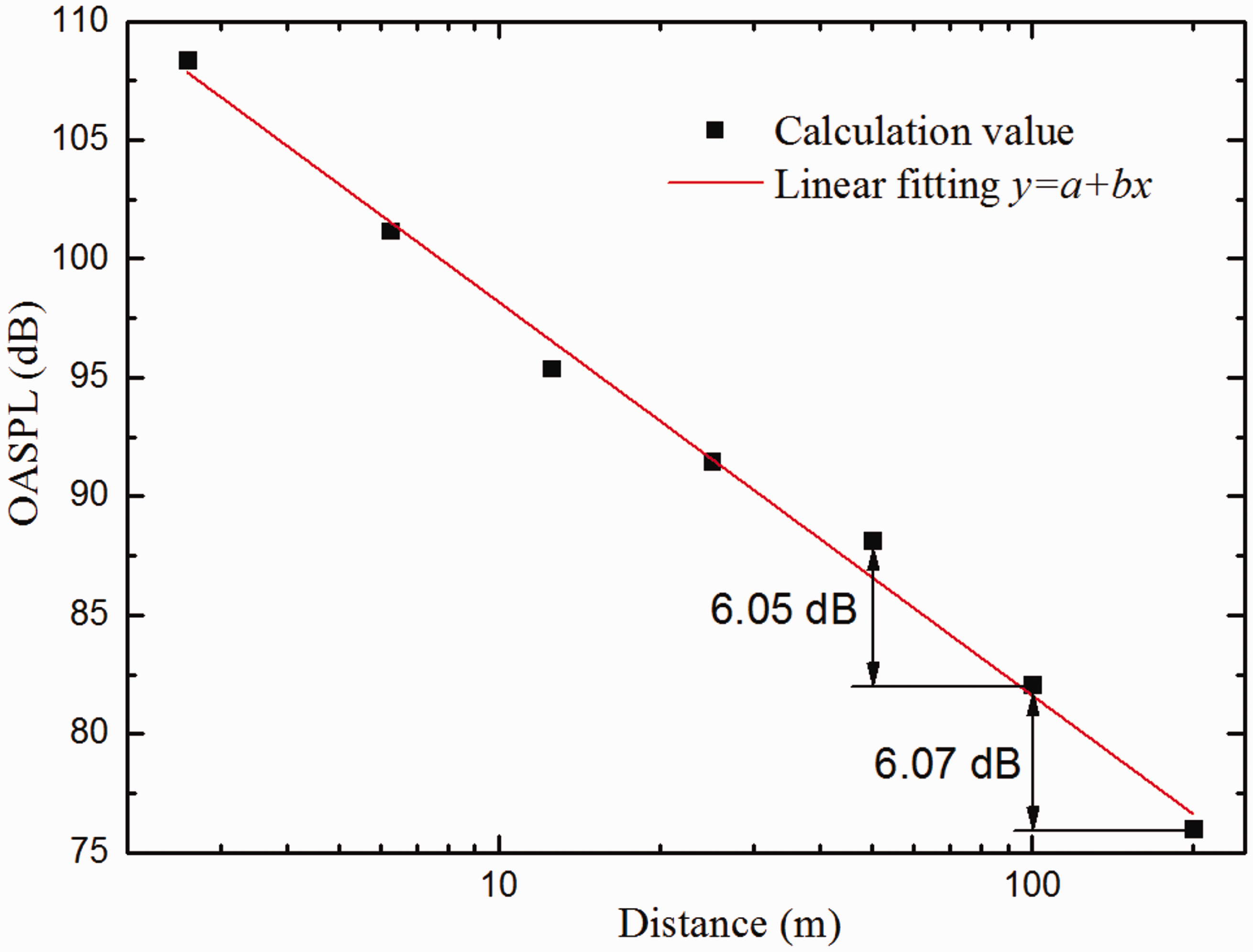
Acoustic attenuation with respect to distance.

Table 4.

Fitting parameters in Figure 17.

Parameter	Value
Equation	y=a+bx
Weight	No weighting
Intercept value	114.716
Intercept standard error	0.872
Slope value	−16.548
Slope standard error	0.574
Statistics adj. R-square	0.993

Reduction of aerodynamic noise in windshield region

In order to control the aerodynamic noise in the windshield area, it is widely used to install outer-windshields at the both sides of the coach to reduce the air-flow into the cavity, so as to reduce the turbulent intensity. In this section, two typical forms of outer-windshields are designed to reduce aerodynamic noise in inter-coach windshield area, as shown in Figure 18. The former is named half-windshield that closed or open baffles are installed on the four sides. Among them, the length and width of the top baffle is 0.2 m and 2.27 m. The length and width of the bottom baffle is 0.1 m and 2.68 m. And the length and width of the baffles on both sides are 0.2 m and 2.23 m. The latter is newly designed and called full-windshield that the inter-coach is smoothly connected with flexible material with the cavity completely isolated. Besides, the folding structure is designed to maintain good tensile and compressive performance. To explore the noise reduction effects of the outer-windshields on aerodynamic noise, both types are studied in this section. Open baffles of the half-windshield are adopted and the fold structure of the full-windshield is kept for actual impacts.

Figure 18.

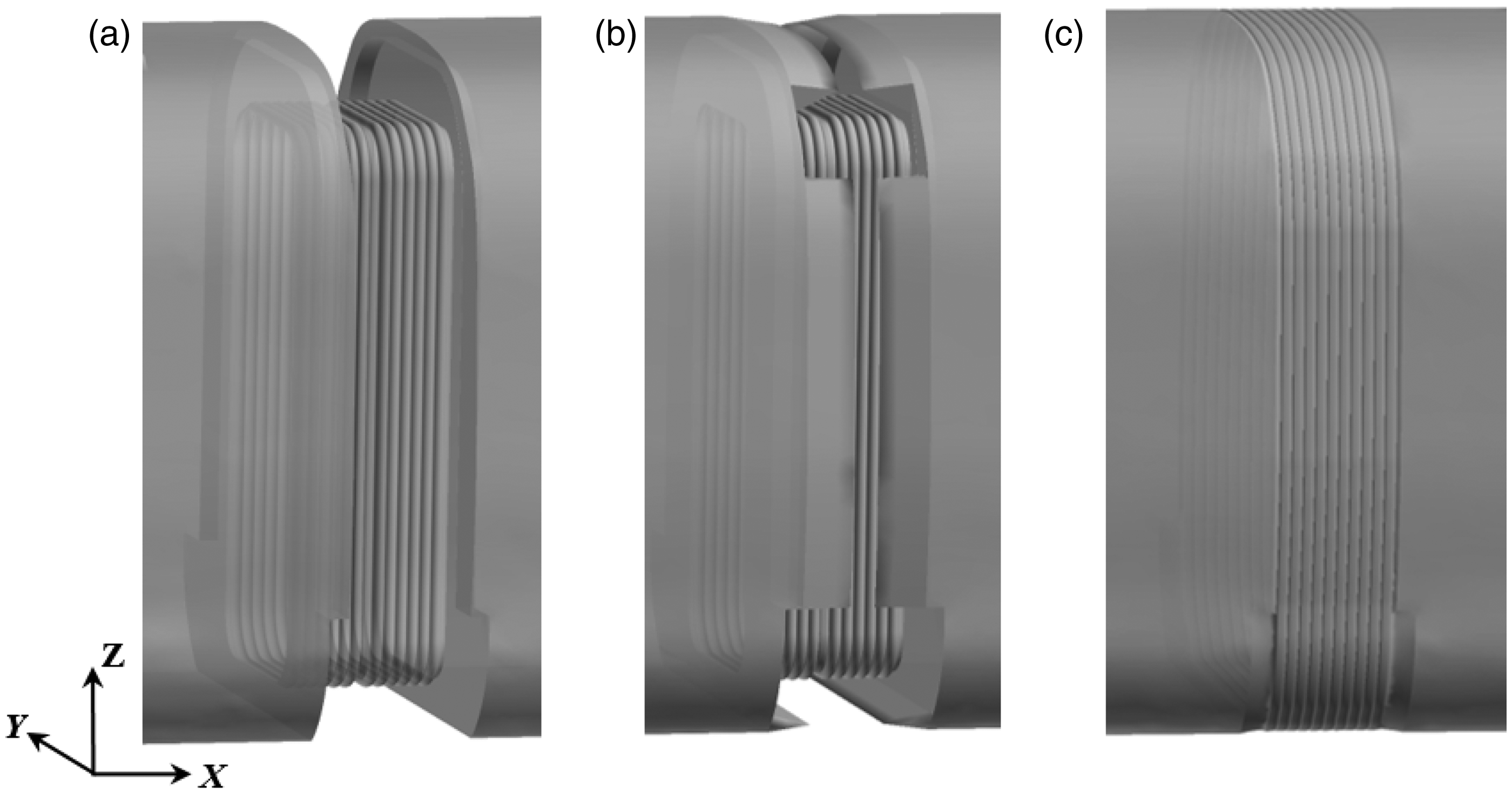
Typical design forms of outer-windshield: (a) original one, (b) half-windshield, (c) full-windshield.

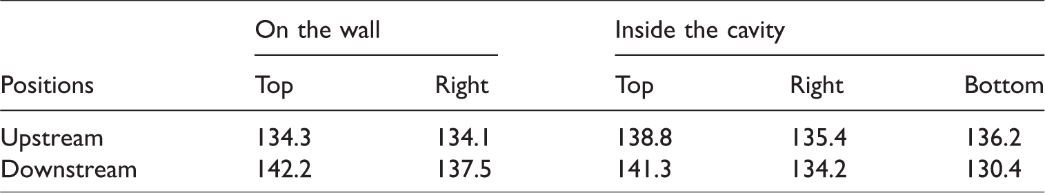
The measuring points are also arranged around the windshield as shown in Figure 11 for aerodynamic noise of the two forms. The OASPL values of measuring points inside the cavity of the half-windshield are listed in Table 5. Compared with the case without baffles (Table 2), the aerodynamic noise inside the cavity of half-windshield is not weakened evidently as expected, while the noise at the top increases by about 6 dB on the contrary. Figure 19 shows the comparisons of one-third octave frequency spectrum of aerodynamic noise inside the cavity at P9 and P10, whose magnitudes are SPL and frequency ranges are from 10 Hz to 5k Hz. The noise of half-windshield at the top is mostly increased in the whole range, corresponding to the larger OASPL. The reasons of noise increasing inside cavity can be summarized into three aspects. Firstly, although open baffles are installed to prevent the airflow from entering the inter-coach space, the airflow feedback inside the cavity is intensified, which means there is more recirculation and the cavity effect is enhanced. Secondly, the airflow would be separated when it reaches the protrusion of the downstream baffle. The protrusion structure is liable to cause the airflow oscillations and vortex falling off, which induces the edge tones, i.e. introduces a new noise source. Thirdly, open baffles are installed upstream and downstream, and the observation points (P9, P10) are closer to the opening of the inter-coach space. Therefore, the airflow disturbance has more obvious impacts on these points. The results above indicate that arrangement of half-windshield is ineffective in reducing the noise inside the cavity. As for the full-windshield form, the cavity is completely isolated and no noise will be generated inside the cavity obviously.

Figure 19.

Comparisons of one-third octave frequency spectrum of the aerodynamic noise inside the cavity in the half-windshield form: (a) P9, (b) P10.

Table 5.

The OASPL inside the cavity of half-windshield (dB).

Positions	On the wall		Inside the cavity
	Top	Right	Top	Right	Bottom
Upstream	134.3	134.1	138.8	135.4	136.2
Downstream	142.2	137.5	141.3	134.2	130.4

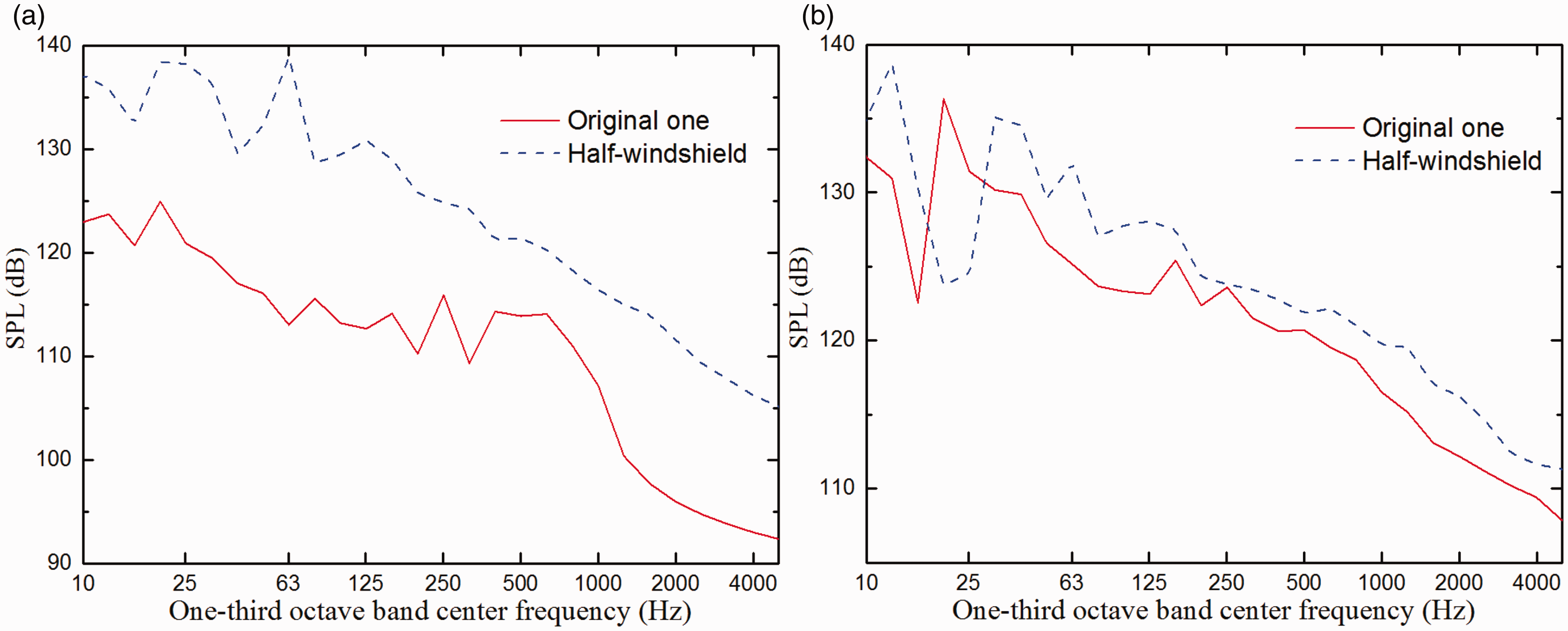
The comparisons of one-third octave frequency spectrum in different windshield forms at P13 and P8 are shown in Figure 20. The spectrum results at P13 indicate that the aerodynamic noise of the half-windshield and full-windshield is relatively close in most frequency range, which is remarkably lower than that of the original one over the whole frequency range. In addition, the OASPL values in different cases are 130.4 dB, 117.5 dB, and 117.1 dB, respectively. The OASPL of the two out-windshield forms at P13 is about 13 dB lower, indicating that both schemes have good effects on reducing aerodynamic noise at the side of the windshield region. The spectrum results at the top (P8) show that aerodynamic noise in the half-windshield case is obviously higher than that in the original case, while the spectrum in the full-windshield case is basically similar to the original one. The OASPL values at the top are 115.8 dB, 124.1 dB, and 114.6 dB, respectively. It is noticed that the OASPL of the half-windshield increases by about 8 dB compared with the original one, indicating that the noise is greatly worsened on the contrary. As for the full-windshield form, the OASPL is slightly reduced by about 1 dB, implying the inconspicuous noise reduction effect. Since there are air-container covers installed upstream and downstream at the top, the airflow disturbance caused by the covers might be as significant as that of the inter-coach space.

Figure 20.

Comparisons of one-third octave frequency spectrum of the aerodynamic noise outside the cavity in different windshield forms: (a) P13, (b) P8.

Further analysis of the noise reduction effect is carried out. In the half-windshield case, the baffles are set on the edges of the coach to reduce airflow into the cavity for noise reduction. The turbulent intensity outside the cavity would be weakened as the baffles increase the smoothness. Even though the level of internal noise becomes relatively higher owing to more intense airflow oscillation inside the cavity, the noise on the side is still effectively reduced due to the shielding effect of baffles. However, as shown in Figure 21(a), the airflow at the top of the windshield becomes more chaotic and the turbulent intensity would increase owing to the air-conditioner covers, as a result the noise reduction of half-windshield is not effective at the top. In the full-windshield case, the surface smoothness of the inter-coach windshield area becomes better and the airflow disturbance becomes smaller, which leads to remarkable noise reduction on the side. Similar to the half-windshield, since turbulent intensity behind the air-conditioner covers is still high as shown in Figure 21(b), the reduction effect at the top is also limited.

Figure 21.

The intensity of turbulent kinetic energy at the top of two typical design forms: (a) half-windshield, (b) full-windshield.

To sum up, both of the windshield forms have effects on the noise reduction on the sides of the windshield region, and especially the full-windshield is better for the interior noise reduction at the inter-coach. In addition, the air-conditioner covers at the top require optimizations of the design and arrangement for further noise reduction.

Conclusions

This study proposes a hybrid numerical methodology of NLAS and FW–H equation to investigate the aerodynamic noise radiated from inter-coach windshield region of high-speed train systematically. Conclusions of the current work are summarized as follows.

The windshield area is one of the main distribution areas of high turbulent kinetic energy around high-speed train. The airflow in windshield region is extremely complicated with significant three-dimensional characteristics, and the flow feedback and oscillations form the noise sources with high energy. The sound pressure distribution on both sides of the windshield area appears symmetrical two-lobe shape, and the dividing boundary is on the upstream edge of the coach.

The acoustic power of aerodynamic noise in the windshield region in the low frequency range below 100 Hz is closely related to the self-excited resonance inside the cavity with a resonance peak frequency of about 42 Hz. The aerodynamic noise inside the inter-coach space is typical broadband noise in the frequency range from 100 Hz to 5k Hz. In addition, most acoustic energy is restricted in the low-medium frequency range below 500 Hz.

The OASPL peaks of the longitudinal near-field noise appear at the position of 3 m away from the windshield, while a trough appears around the windshield region instead. The distribution characteristics are closely related to the aerodynamic noise sources interferences and the locations of the bogies and the air-conditioner covers. Meanwhile, the OASPL values of aerodynamic noise in the windshield region are demonstrated to grow logarithmically with the train speed, and the acoustic power approximately grows as the 5^th power of the speed. The propagation of the aerodynamic noise radiated from the windshield region can be considered as the cylindrical waves radiation of two line sound sources in the near-field, but in the far-field it is primarily in the form of the spherical wave.

Both of two typical forms of outside-windshields have evident effects on the reduction of the aerodynamic noise radiated from the sides of the windshield region, and the noise reduction effects at the top are greatly limited due to the air-conditioner covers. However, the half-windshield has no effect on the interior cavity noise reduction, while the full-windshield apparently eliminates the generation of inside cavity noise. Therefore, the full-windshield is recommended to be installed at the inter-coach space to lessen aerodynamic noise of the windshield region. The shape and installation location of air-conditioner covers at the top require optimization for further noise reduction.