Sage Journals: Discover world-class research

Abstract

In modern hospitals, monitoring patients’ vital signs and other biomedical signals is standard practice. With the advent of data-driven healthcare, Internet of medical things, wearable technologies, and machine learning, we expect this to accelerate and to be used in new and promising ways, including early warning systems and precision diagnostics. Hence, we see an ever-increasing need for retrieving, storing, and managing the large amount of biomedical signal data generated. The popularity of standards, such as HL7 FHIR for interoperability and data transfer, have also resulted in their use as a data storage model, which is inefficient. This article raises concern about the inefficiency of using FHIR for storage of biomedical signals and instead highlights the possibility of a sustainable storage based on data compression. Most reported efforts have focused on ECG signals; however, many other typical biomedical signals are understudied. In this article, we are considering arterial blood pressure, photoplethysmography, and respiration. We focus on simple lossless compression with low implementation complexity, low compression delay, and good compression ratios suitable for wide adoption. Our results show that it is easy to obtain a compression ratio of 2.7:1 for arterial blood pressure, 2.9:1 for photoplethysmography, and 4.1:1 for respiration.

Keywords

biomedical signals large-scale health data compression downsampling variable length coding

Introduction

The global datasphere increases at a compound rate of 24%, and it is predicted to reach nearly 180 Zettabytes by 2025.¹ While the actual distribution between data storage and data generation averages 1 to 49 ratio, in Healthcare, the ratio is 1 to 2.35,² meaning that the future health data generation possibility is vast and untapped today. Indeed, such a remarkable difference contributes to the reported annual compound growth specific to the global health datasphere: 36%, which is 50% larger than the global average. Wearable, non-invasive, Internet of medical things (IoMT), and big data analytics technologies contribute to more data being collected. In a society envisioned by the European Commission, flowering under the umbrella of the European Health Data Space (EHDS) regulation,³ efficient data collection and storage will be a sine qua non-condition to see the future outlined by the EHDS, where progress is driven and sustained by access to health data.

Understanding the characteristics of biomedical big data can be considered the most critical requirement for harnessing the true potential of health data.⁴ Biomedical signals, such as the electrocardiogram (ECG) signal has long been used for diagnosing cardiac complications⁵ or as a vital sign in intensive care.⁶ Using methods, such as signal processing or machine learning, we are now starting to understand that these continuous measurements carry more important information than what we know today. This does not only hold for ECG. Recently, Davies et al.⁷ and Lee et al.⁸ have shown that during surgery, the shape of the arterial blood pressure (ABP) curve can be used to predict the onset of hypotension ahead of time. Using sensor-fusion of multiple biomedical sensors, van der Ster et al.⁹ reported a prognosis of hypovolemic shock before blood pressure starts to drop. Hence, curve data contain information revealing important clinical facts and must be collected and stored without loss of information.

Many biomedical signals are routinely measured continuously, generating time-series data, sometimes called high-frequency or curve data. Typical signals include ECG, ABP, photoplethysmography (PPG or sometimes PLETH), and respiration (RESP). Depending on the patient need, many more signals can be collected. However, storing all patient-generated data can be a challenge as typical hospitals may have several thousands of patients. Many of them will have one or more sensors. At the same time, data storage at hospitals needs high reliability and privacy protection due to patient safety and regulations, which makes storing large amounts of data expensive and cumbersome.

The focus of this article is to investigate the compression of biomedical signals for large-scale collection and storage of biomedical signals. Since there is a large body of research regarding the compression of ECG,¹⁰ this article will focus only on compression of the remaining biomedical signals; in particular ABP, PPG, and RESP. The aim is not to propose yet another compression method with an minor compression improvements, but to validate several simple compression methods to these biomedical signals and identify the best available technique and configuration for each of them. However, the sometimes subtle changes in the signal should not be accidentally removed by the digitalization process and/or compression, since it is not known whether those subtle changes carry essential information. Therefore, we will mainly investigate lossless and near-lossless compression algorithms.

State of the art

There are numerous examples of ECG signal compression,^10–15 consisting of multiple time series due to the many leads usually involved in medical ECG measurements. However, compression for other biomedical signals is almost non-existent in comparison. One exception is Gogna et al.,¹⁶ which compresses both ECG and electroencephalogram (EEG) signals. Other exceptions are Banerjee and Singh,¹⁷ where lossless compression methods for ECG and PPG signals are proposed, and Nakatsuka et al.,¹⁸ where compression of the less common signals; intravesical pressure and rectum pressure are investigated. Some papers^19,20 propose compression methods for electromyography (EMG) signals.

There are too many papers covering compression of ECG signals to mention them all here.¹⁰ Most proposed lossless compression methods^13–15 are based on linear prediction followed by coding the residual errors using variable length coding, such as Huffman or Golomb-Rice codes. In some proposals,¹³ adaptive linear prediction is used where the prediction coefficients adapts to the signal for improved compression over time. Another approach is to use a transform-based approach, such as the one by Arnavut.¹¹

When it comes to lossy ECG compression, transform-based approaches are very common.¹² Discrete Cosine Transform (DCT) is one way to perform lossy ECG compression as proposed by many authors.^21,22 Ranjeet et al.²² explored the possibility of using the Discrete Fourier Transform and the Discrete Wavelet Transform, with the conclusion that all transforms can be used for compression while preserving necessary clinical information. Compressed sensing (CS) is another method that combines random sampling and the potential sparsity of a signal by sampling at sub-Nyquist rates and still reconstructing the original signal. Many authors^12,16 have proposed CS for compressing ECG signals.

Gogna et al.¹⁶ proposed to use a type of artificial neural network (ANN) called a stacked autoencoder for compressing ECG and EEG signals. They also proposed to extend the ANN for compression with classifier outputs for automated diagnosis of some common cardiac complications when used on ECG signals.

Not only compression is important, but also many other system aspects. The Hospital for Sick Children (HSC), Toronto, Ontario, Canada, developed a database named Atrium that stores, compresses, and retrieves physiological signals from one of its departments.²³ AtriumDB is vendor-neutral and integrates with existing bedside monitors. It uses lossless compression based on differential pulse code modulation (DPCM) and BZip2. Metadata is stored in a relational database, and signals are divided into 10-min segments and stored in a file system to allow for more efficient data handling, storing, and retrieval.

Biomedical Signals

Today’s hospital settings use extensive monitoring, such as perioperative care and intensive care, where biomedical signals are gathered with multiple leads or sensors. They are immediately digitized using an analog to digital converter (ADC) before being connected to a bedside monitor for feedback to the acting specialist or nurse. The digital signal may also be transferred to a central office, where all patients in the department are monitored simultaneously. Finally, the signal data may be sent to a hospital-based database for storage and future analysis, but that is not yet common practice.

Most biomedical signals are sampled with a 100-500 Hz sampling rate and an 8-16 bits ADC. The ADC will read the instantaneous amplitude and convert into a integer with a certain bit length. A longer bit length means better resolution, but also require more storage space. In pulse code modulation (PCM), every sampled value is stored as a long sequence of integers. Sometimes the curves are saturated by the upper and lower limits, and sometimes, they only utilize part of the full range of the ADC. Nevertheless, to store these values using 16-bit integers per sample is common, even when sampled with a 10 or 12-bit ADC. This by itself is a waste of storage space. Furthermore, the sampling rate is much higher than needed for many biomedical signals, that is, they are oversampled. Power spectral analysis of the biomedical signals reveals that many signals do not have high-frequency components and can be sampled with lower sample frequency, as long as not lower than the Nyquist rate (twice the frequency of the highest frequency component). For instance, the power spectrum of the ABP waveform shows that very little power exists in frequencies above 25 Hz, meaning that a sampling rate of 50 Hz is sufficient. Hence, a straightforward way to reduce storage requirements is to use a lower sampling rate or downsample if the signal is already sampled. The latter is possible by applying a low-pass filter followed by only saving every M:th sample. If the Nyquist requirement is still fulfilled, no essential information loss will occur.

The amount of compression possible for a medical signal depends on the signal characteristics, the sample rate, and the ADC bit-resolution. Typically, we measure the compression ratio (CR) as the fraction between the uncompressed bits and the compressed bits. Typical lossless compression methods of ECG signals of 360 Hz with 11-bits ADC have a CR range between 1.9:1 and 2.4:1, depending ECG channel and the used compression method.¹³ This can be compared to reducing the sample rate from 360 Hz down to 125 Hz, which corresponds to a CR of 2.88:1. However, such a downsampling is of course not lossless.

HL7 Fast Healthcare Interoperability Resources (FHIR)²⁴ is an important health data standard that also defines how to transfer sampled data. However, FHIR specifies that sampled data should be transferred as space-separated integers coded as decimal numbers using ASCII characters. This means that the data transfer will be significantly larger than the uncompressed raw values. Typically, every sampled value will be represented by 5 bytes (including the space character). Hence, HL7 FHIR is not optimized to deal with large amounts of sampled data.

Methods

In this article, we will apply simple compression to different signal types in order to investigate the amount of compression that can be achieved. We will experiment with some common methods and try the relevant configurations for them in order to find the typical compression performance. The following sections will first discuss different lossless compression methods followed by a downsampling method. All methods will work for any biomedical signal, but their compression ratios will differ.

Lossless methods

Lossless compression for time-series data is usually based on reducing the variance of the values and then giving more frequently occurring values a shorter code. The latter is called variable length coding (VLC), which we discuss in a later subsection. A simple way to reduce variance is differential pulse code modulation (DPCM), which is the same as recalculating the sampled values x(n) as follows:

y (n) = x (n) - x (n - 1)

(1)

DPCM can also be said to predict the next value based on the previous value, i.e., $\hat{x} (n) = x (n - 1)$ . The prediction $\hat{x} (n)$ will have a prediction error, usually called a residual error e(n) that needs to be coded:

e (n) = x (n) - \hat{x} (n)

(2)

The errors e(n) are clustered around 0 and their variance is hopefully small. This will lead to efficient compression when combined with an efficient VLC. Another straightforward, yet effective, method is to use the trend to predict future values, i.e.:

\begin{array}{l} \hat{x} (n) & = x (n - 1) + Δ x (n - 1) \\ Δ x (n - 1) & = x (n - 1) - x (n - 2) \end{array}

(3)

which we will call the linear trend prediction. The two previous methods can be generalized as linear predictions using the following equation:

\hat{x} (n) = \sum_{k = 1}^{M} h_{k} x (n - k)

(4)

where h_k are the predictor coefficients. If not all h_k are integers, we need to round equation (4) to the nearest integer. Equation (4) is known as a finite impulse response (FIR) filter.

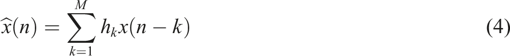
To use equation (4) for DPCM, we just set M = 1 and h₁ = 1. For the linear trend prediction, we have M = 2, h₁ = 2, h₂ = −1. However, there may be better parameter configurations given the curve data, which we may try to find with optimization tools or machine learning.

Variable length coding

In variable length coding (VLC), each value is given codes of different lengths depending on the frequency of occurrence, where common values are given codes with shorter lengths. VLC will achieve a good compression ratio if a few values are very common.

In Huffman coding, you first go through all your values to check the frequency of every occurring value. An optimal code list is created in the form of a Huffman tree. This is the optimal VLC, but the Huffman tree needs to be coded too and added to the compressed values as overhead. Furthermore, it must pass through (at least part of) the sequence before the (semi-)optimal Huffman tree can be created and the compression starts. If we want to compress short sequences of values or reduce compression delay, we need to avoid Huffman.

Another popular method is Golomb-Rice codes²⁵ or a variant called Exponential-Golomb.¹⁸ In our case, Exponential-Golomb is always more efficient, so we focus on only that variant. Exponential-Golomb only encodes positive integers larger than 1, and assigns smaller codes to smaller values. Since our residual errors are small and scattered around zero, we first need to convert them into positive integers as follows:

y = {\begin{cases} - 2 x & x \leq 0 \\ 2 x - 1 & x > 0 \end{cases}

Exponential-Golomb has a parameter called order: k. It means that the k least significant bits are coded with normal binary coding and only the remaining bits are encoded with variable length codes. If we start with a positive integer y, we code y mod 2^k in binary format as usual. For the remaining bits, we add 1 to make it larger than zero: y′ = ⌊y/2^k⌋ + 1. Then we count the number of bits in y′, that is, n = ⌊ log₂y′⌋ + 1. The code is formed by a prefix of n zeroes followed by binary codings of y′ and y mod 2^k. The first part ensures that one code is never the prefix of another code, which is important for decompression. The number of prefix zeroes gives the number of bits for y′ and k gives the number of bits of the last part.

Downsampling

A very efficient way to reduce the space requirement is to downsample an already digitized signal if it is sampled at a high rate.¹⁴ The process of reducing the sampling rate consists of two steps, where the first being a low-pass filter to avoid aliasing (distortion). The filter must remove any frequency components higher than half the new sample rate (i.e., the Nyquist frequency). In the second step, samples are removed and this will reduce the storage size requirement, but also remove signal information. After downsampling, we can compress further using any of the lossless methods, but with reduced compression ratio as there are much less redundant information.

In our implementation, we keep every N:th samples, where $N \in Z^{+}$ . The anti-aliasing filter is a Chebyshev type II filter design, which has a flat response in the pass band. We used order 8 and a cut-off frequency set to the Nyquist frequency multiplied with a factor of 1.1 in order to preserve frequencies close to the Nyquist frequency, but still attenuate at least −40 dB beyond the Nyquist frequency. A forward-backwards filter was used to avoid unnecessary phase shifts.

Experimental setup

We conducted experiments on pre-recorded data to test the compression methods on real biomedical signals. In this section, we introduce the evaluated methods, the performance metrics, and the used data.

Evaluated methods

In the remaining of this article, the focus is on the following compression methods:

• DPCM according to equation (1)

• Trend, which is the linear trend prediction in equation (3)

• LinP(k), which is the general linear prediction of equation (4) with either order M = 3 or 4. The h_k parameters are determined from a separate set of data as mentioned in the Results section.

• Down(N), which is the downsampling method mentioned earlier

All the above are combined with VLC approaches, namely Huffman, Golomb-Rice, Exponential-Golomb coding with order k, and Lempel-Ziv-Welch (LZW). The Huffman coding requires two passes of data and the resulting Huffman tree also needs to be stored. However, the storing of the Huffman tree is ignored. Therefore, we mainly consider this option as a theoretical upper limit of what VLC can achieve. Golomb-Rice and Exponential-Golomb coding with order k are not optimal, but has no overhead and is close to what can be achieved. LZW is included for comparison only. In the Results section, we tune the order parameters for the different methods and signals to maximize the compression ratio.

Performance measurements

The main measurement in this work is the compression ratio (CR), which can be expressed as the fraction between the uncompressed bits and the compressed bits, where a higher number means more compression. As uncompressed bits, we assume a compact storage of the PCM values. I.e., if the signal is sampled with an ADC of 12 bits, we assume that they are stored as 12-bits binary values. In practice, this is rarely the case. Instead, 12-bit values are typically stored as 16-bits values, such as most of the MIMIC-3 wfdb data,^26,27 or as whitespace-separated (or comma-separated) ASCII-coded decimal numbers as with FHIR. Going from 16-bit to 12-bit values represents a compression ratio of 1.33:1 and going from a FHIR storage to 12-bits values gives an approximate compression ratio of 3.3:1. These numbers should be multiplied with the reported compression ratios below if compression from those storage methods is considered.

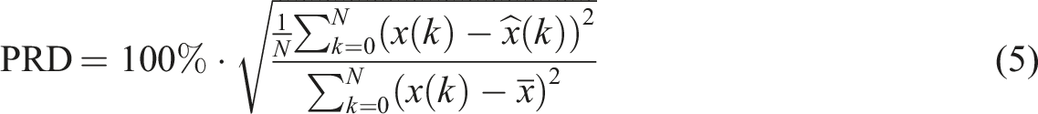
For the downsampling method, it is also necessary to measure the amount of information loss introduced by the filtering and downsampling steps. We reconstruct the signal to the original sampling rate by interpolating removed samples using a polyphase filter based on Kaiser with β = 5. Then the quality of the reconstructed signal is compared to the original signal. The quality reduction is calculated as the Percentage Root Mean Square Difference (PRD) as specified in the equation (5):

P R D = 100 % \cdot \sqrt{\frac{\frac{1}{N} \sum_{k = 0}^{N} {(x (k) - \hat{x} (k))}^{2}}{\sum_{k = 0}^{N} {(x (k) - \bar{x})}^{2}}}

(5)

where x(k) is the original signal,

\hat{x} (k)

is the signal after filtering, downsampling, and reconstruction, and

\bar{x}

is the mean value of all original signal values. A PRD close to 0% is considered a very good value. Pearson correlation coefficient, r, is also calculated, which is very close to 1. Therefore, 1 − r is instead reported, which should be as small as possible. Another popular metric is normalized root-mean-square error (NRMSE), which is similar to PRD and therefore will not be used in this article.

Test data

For the validation of the compression methods, we used biomedical signal data from version 1.0 of the MIMIC-III Waveform Database (WFDB).^26,27 The database contains vital signs recordings from approximately 30,000 ICU patients from several U.S. hospitals. It is a de-identified dataset and is made public under the Open Data Commons Open Database License v1.0, which we adhere to. Requirement for patient consent was not needed because it did not impact clinical care and all data was de-identified. Under the US Health Insurance Portability and Accountability Act (HIPAA), this means research using this data does not constitute human subjects research. The same holds for the authors’ national ethical review authority.

For this study, we selected ABP, PPG, and RESP only. Those signals are sampled at 125 Hz using an ADC of either 8, 10, or 12 bits. We decided to ignore recordings of 10 bits and only focus on 8 and 12-bit recordings. Furthermore, there were very few 8-bit recordings of respiration, so we excluded that too.

The MIMIC-III WFDB contains the raw sampled data of vital sign waveforms, including noise, motion artefacts, and sometimes just nonsense data due to many different types of recording problems. However, this is typical for vital sign data being recorded at hospitals. Since it is difficult to determine whether a signal is good, it is better to collect and store everything. Because of this, it is important that the compression methods also can deal with this real-world data, which is an important part of the validation. Hence, we have not attempted to remove any noise as long as there is not only noise for a particular biomedical signal from a particular patient.

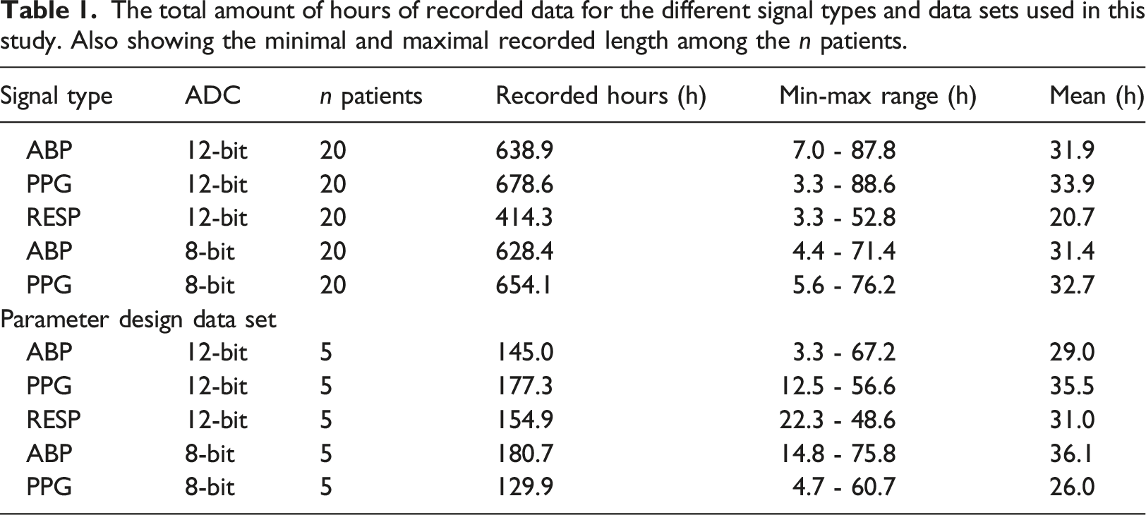
Using the Python WFDB API, signal data from 20 random patients for each signal type were identified and downloaded. Each patient recording was subdivided into segments by MIMIC. We excluded patients with less than 3 h of recorded values or more than 100 h to achieve some balance between the patient recordings. This exclusion will not alter the distributions in any significant way, since the signals share the same distribution regardless of the recorded signal length. Segments shorter than 10 s or containing data with zero variance were also removed, since they usually only contain noise or nonsense values. Since the latter is such a small amount of data compared to the total (maximum was 1% for 12-bit RESP), it will have a very marginal effect on the final results.

For finding the best parameters for some of our methods, we downloaded a separate data set in the same way as above, but only 5 patients. Table 1 lists the two data sets and the data they contain.

Table 1.

The total amount of hours of recorded data for the different signal types and data sets used in this study. Also showing the minimal and maximal recorded length among the n patients.

Signal type	ADC	n patients	Recorded hours (h)	Min-max range (h)	Mean (h)
ABP	12-bit	20	638.9	7.0 - 87.8	31.9
PPG	12-bit	20	678.6	3.3 - 88.6	33.9
RESP	12-bit	20	414.3	3.3 - 52.8	20.7
ABP	8-bit	20	628.4	4.4 - 71.4	31.4
PPG	8-bit	20	654.1	5.6 - 76.2	32.7
Parameter design data set
ABP	12-bit	5	145.0	3.3 - 67.2	29.0
PPG	12-bit	5	177.3	12.5 - 56.6	35.5
RESP	12-bit	5	154.9	22.3 - 48.6	31.0
ABP	8-bit	5	180.7	14.8 - 75.8	36.1
PPG	8-bit	5	129.9	4.7 - 60.7	26.0

Results

The results in this section are based on calculations and simulations implemented in Python 3 and NumPy. In the first part, we find the best parameters for some of the methods based on the parameter design data set. Then, we apply the methods with their parameters on the validation data set to see how efficient the different compression methods perform on the MIMIC-III WFDB data.

Finding the optimal predictor coefficients

The first step was to find the best predictor coefficients in equation (4) for the methods LinP(3) and LinP(4). The optimal coefficients are different for different types of signals and ADC bit depths, so we searched for each of the five combinations on the parameter design data set. The minimization function is the achieved length of the compression of all the recorded signal values of the given type from the parameter design data set. The coefficients are provided as a vector, and we used Exponential-Golomb with order k = 0 as the VLC. The modified Powell search algorithm was used and we tried several initial values to increase the likelihood of finding the global minima. However, the function is not smooth, and a local minimum was often found.

Table 2 lists the found optimal coefficients for all signal types and ADC bit-depths. It can be seen that for respiration, no other set of prediction coefficients could be found besides the ones used by the Trend method. The reason could be that the respiration curve data is too erratic and unpredictable. For the ABP signal types, no better set could be found for M = 4 coefficients compared to M = 3 coefficients.

Table 2.

Linear predictor coefficients for order 3 and 4 for all signal types and ADC bit-lengths.

Signal type	ADC	h ₁	h ₂	h ₃	h ₄
Predictor coefficients h_k for order M = 3
ABP	12-bit	2.739	−2.519	0.780
PPG	12-bit	2.837	−2.694	0.857
RESP	12-bit	2	−1	0
ABP	8-bit	2.494	−2.107	0.613
PPG	8-bit	1.99	−1.073	0.083
Predictor coefficients h_k for order M = 4
ABP	12-bit	2.739	−2.519	0.780	0
PPG	12-bit	2.712	−2.305	0.452	0.141
RESP	12-bit	2	−1	0	0
ABP	8-bit	2.494	−2.107	0.613	0
PPG	8-bit	2.004	−1.073	0.050	0.019

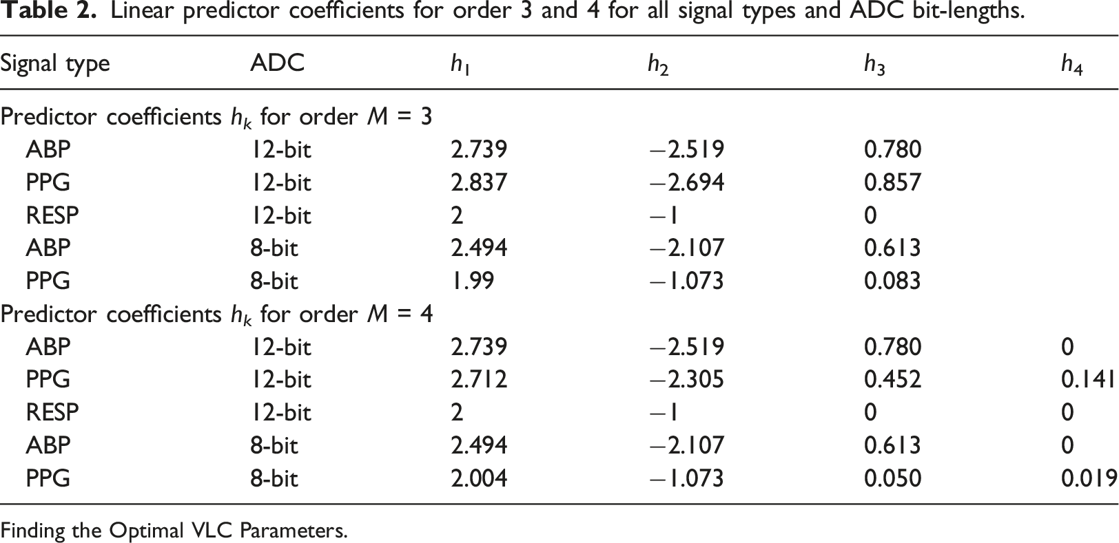
Finding the Optimal VLC Parameters.

The second step was to determine the best parameters for the different VLCs. We started with the Exponential-Golomb order k parameter and tried different values of k in the expected range 0 ≤ k ≤ 6. We calculated the average compression ratio for LinP(3) and LinP(4) to see which order k gives the best results. This was done per signal type, and the results of this from the parameter design data set are shown in Figure 1.

Figure 1.

Different order of Exponential-Golomb coding for various 12-bit signals. CR shows the average between LinP(3) and LinP(4).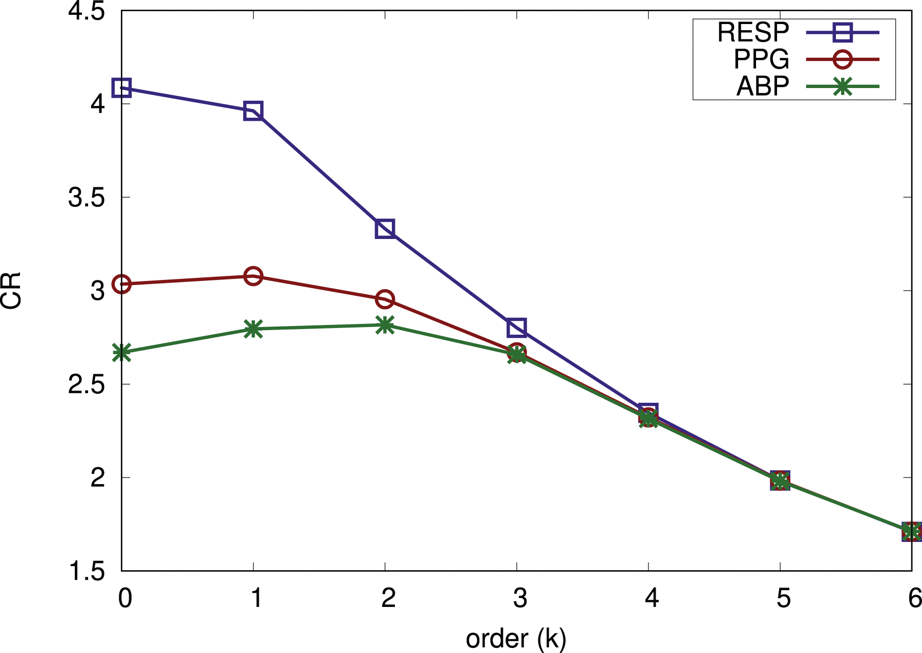

As can be seen in Figure 1, k = 1 is a good trade-off for signals sampled with 12-bits ADC. For respiration, k = 0 is better and for ABP, k = 2 is better. However, the gains are small and we believe it is better to keep parameter choices as similar as possible. Hence, we selected k = 1 for all 12-bit signals. The results for the 8-bit signal types are not shown. It is rarely the case for them that an Exponential-Golomb order larger than 0 is beneficial for the compression ratio. Hence, we use order k = 0 for both 8-bit signals. We also determined the best parameter configurations for Golomb-Rice and LZW in a similar way. For Golomb-Rice, b = 3 was best. For LZW, it was START_BITS = 8 and MAX_BITS = 12 that gave the best compression results.

Then we compared the different VLC methods with each other and this is shown in Figure 2 based on the validation data set. The error bars show the 95% confidence intervals. We show Exponential-Golomb with k = 1 for 12-bit signals and k = 0 for 8-bit signals. As expected, Huffman results in the biggest compression ratio for all types of signals. We also see that Exponential-Golomb is the second-best option for all signal types. Therefore, we will focus on Huffman and Exponential-Golomb.

Figure 2.

The compression ratio for some different VLC methods.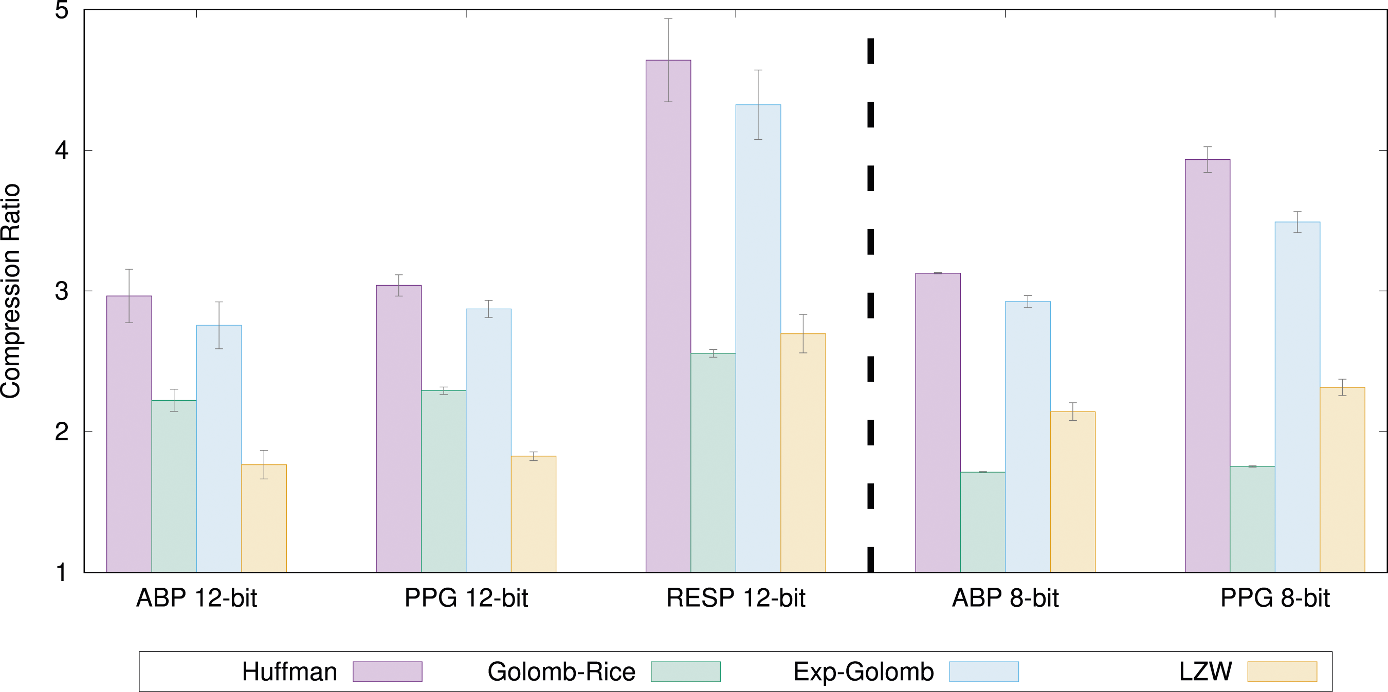

Linear prediction compression

In Figure 3, we show the compression ratio results of all the linear prediction methods on all biomedical signals types. The bars show the average compression ratio of all signal recordings from all n = 20 patients. The error bars show the 95% confidence intervals. The colored bars illustrate the compression ratio for the linear prediction method in combination with Exponential-Golomb with the found best order. The white bars above indicate how much more can be achieved if Huffman coding (excluding overhead) is used.

Figure 3.

The compression ratio of all linear prediction methods for all signals.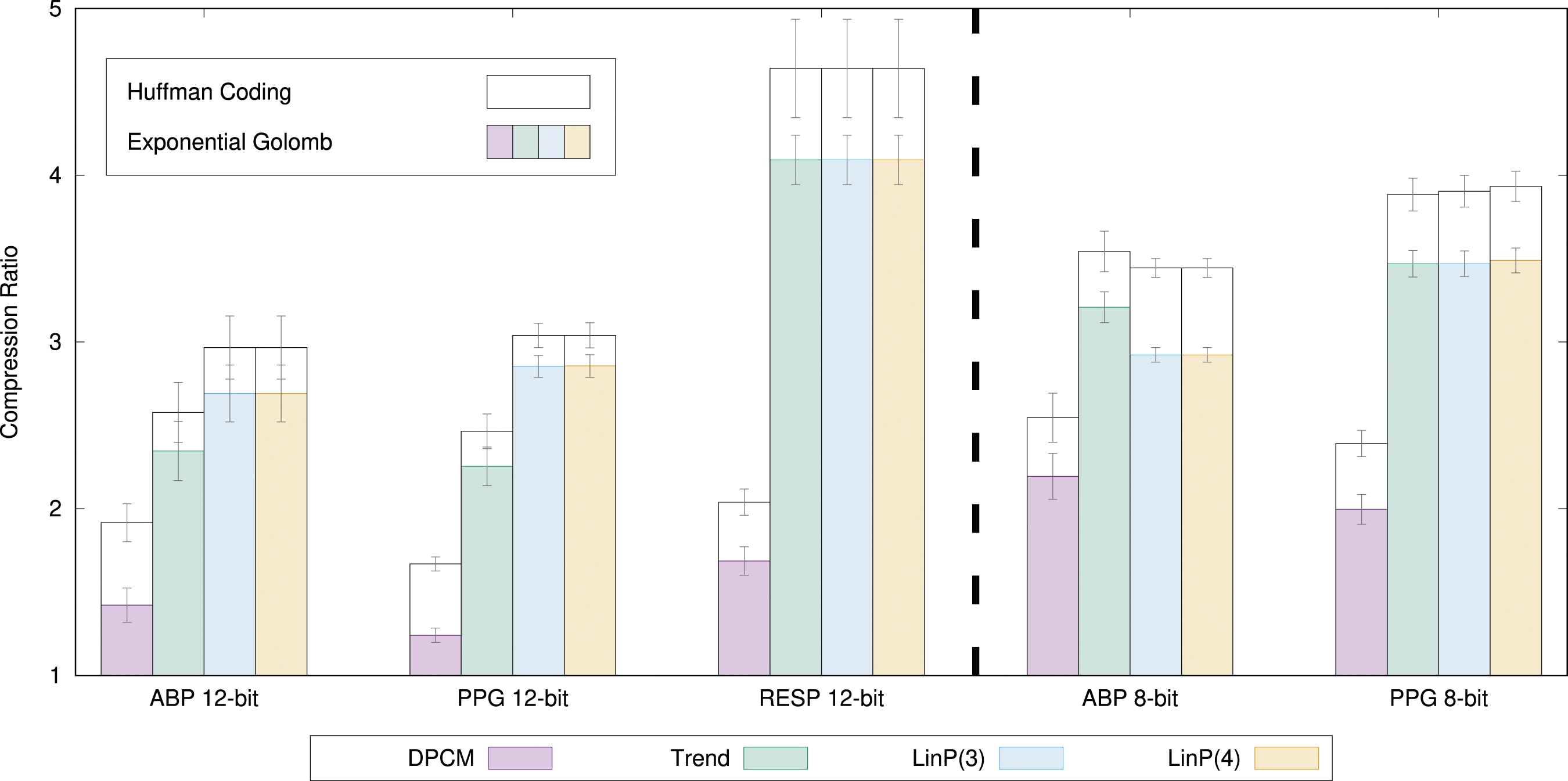

From the results of Figure 3, we can see that, in general, the more complex linear the prediction method, the better the compression ratio. However, there are a few exceptions. For 8-bit ABP, the LinP(3) and LinP(4) methods are worse than Trend, which is not intuitive. This is likely because the prediction coefficients were found from a different data set and are not optimal on the validation data set. This demonstrates the difficulty in designing appropriate prediction coefficients.

Downsampling results

Finally, we studied the compression ratio of downsampling. Since we filter the signal and remove every N:th sample, this is a lossy compression method as we cannot reconstruct the original signal in a perfect way. Figure 4

Figure 4.

Compression results for downsampling the 12-bit signals and using LinP(3) together with Exponential-Golomb (k = 1) or Huffman.

shows the results using LinP(3) and either Exponential-Golomb (k = 1) or Huffman on the downsampled signals. Every dot represent a value Down(N), where N increases and are shown next to the dots. The x-axis represents the information loss measured as PRD (equation (5)). The corresponding maximum Pearson correlation coefficients in the figure are 1 − 5.2 ⋅ 10⁻⁴ for ABP (N = 4), 1 − 3.1 ⋅ 10⁻⁴ for PPG (N = 6), and 1 − 2.8 ⋅ 10⁻⁴ for RESP (N = 14). The compression ratio is a combination of the reduction based on the removal of samples (N:1) and the compression achieved by LinP(3) followed by Exponential-Golomb (k = 1) or Huffman.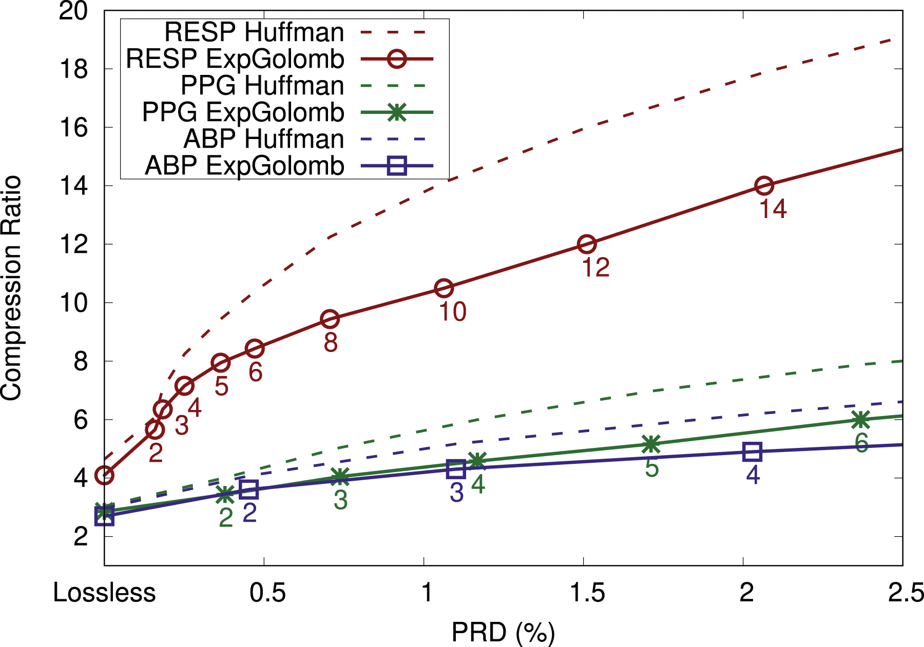

The process of downsampling means that we get different discrete signals and that different predictor coefficients are optimal compared to the non-downsampled signals. Hence, we again used the parameter design data set to find optimal predictor coefficients for each of the signal types and each of the downsampling amounts N. For heavily downsampled signals, a higher order k used by Exponential-Golomb would be more beneficial, but we stick to k = 1 (k = 0 for 8-bit signals) in order to make a solution for most signals. The drawback of always using k = 1 can be seen in that the gap between the Exponential-Golomb curve and the corresponding Huffman curve is increasing as more downsampling (a higher N) is used. Hence, with more tuning, higher compression ratios can be achieved. Since we did not fully tune all parameters, we assume no compression if the compression ratio drops below 1:1, which happens for heavily downsampled signals in Figure 4.

Discussion

When choosing a compression method for biomedical signals, it is important to consider whether one wants a single method for all signal types or whether the best method for each signal type can be considered. Table 3 summarizes the compression results for all signal types and the key compression methods. For downsampling, we assume that a reconstruction error of PRD

\leq 1.0 %

is acceptable and then select the option with the best compression ratio, that is, the highest possible N. The table includes the resulting N and the actual PRD for the downsampling. r is the Pearson’s correlation coefficient. Since all r:s are very close to 1, 1 − r is presented instead, where a smaller value means higher correlation between the original signal and the reconstructed signal.

Table 3.

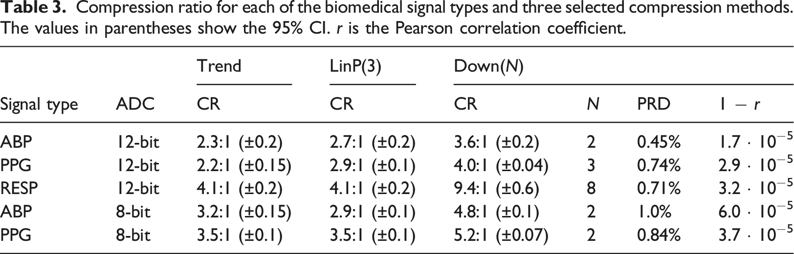
Compression ratio for each of the biomedical signal types and three selected compression methods. The values in parentheses show the 95% CI. r is the Pearson correlation coefficient.

Signal type	ADC	Trend	LinP(3)	Down(N)
Signal type	ADC	CR	CR	CR	N	PRD	1 − r
ABP	12-bit	2.3:1 (±0.2)	2.7:1 (±0.2)	3.6:1 (±0.2)	2	0.45%	1.7 ⋅ 10⁻⁵
PPG	12-bit	2.2:1 (±0.15)	2.9:1 (±0.1)	4.0:1 (±0.04)	3	0.74%	2.9 ⋅ 10⁻⁵
RESP	12-bit	4.1:1 (±0.2)	4.1:1 (±0.2)	9.4:1 (±0.6)	8	0.71%	3.2 ⋅ 10⁻⁵
ABP	8-bit	3.2:1 (±0.15)	2.9:1 (±0.1)	4.8:1 (±0.1)	2	1.0%	6.0 ⋅ 10⁻⁵
PPG	8-bit	3.5:1 (±0.1)	3.5:1 (±0.1)	5.2:1 (±0.07)	2	0.84%	3.7 ⋅ 10⁻⁵

As we demonstrated in this article, there are differences between the signal types. For LinP(3), one would have to select different h_k parameters for the different signal types to get good compression results. However, both Trend and LinP(3) are good options for all signals and achieve good compressions. Furthermore, a lossy method can be considered if one can tolerate some reconstruction errors. In this article, we tried only a downsampling method, but there are options for lossy compression methods available elsewhere, such as methods based on transforms and/or compressed sensing.^12,16 However, such solutions usually need to be tuned differently to the different signals, which adds significant complexity to a final solution.

Nevertheless, the compression ratio is not the only aspect to consider. While Huffman coding would increase the compression ratio considerably, we still argue that it is not a good option as it requires two passes over the recorded data, which would add a considerable amount of compression delay, that is, the time between reading the value and the time it is compressed and sent or stored. Furthermore, the Huffman tree needs to be encoded, which adds overhead. The other approaches have a smaller compression delay. The current downsampling method uses a forward-backwards anti-aliasing filter, which adds significant compression delay, while the linear methods only have 2-4 samples delay (16-32 milliseconds). Finally, low complexity computations are also necessary, enabling implementations also on simple cheap battery-less wearables.

In summary, we find the linear prediction with order M = 3 combined with Exponential-Golomb with k = 1 to be a good candidate due to the trade-offs mentioned above. Increasing the order from 3 to 4 in the linear prediction only leads to a slight improvement, and we do not expect much more improvement for order 5, which is confirmed by Deepu and Lian.¹³ Linear prediction can achieve a good compression ratio and is very simple to implement and compute. It could work well in hospital-wide biomedical signal collection and storage systems and should be a good candidate for the standardization of such protocols and systems. As a one solution for everything, it offers a good trade-off and simplifies wide adoption.

The focus of this study was to investigate the compression of biomedical signals for large-scale collection and storage, which will accelerate in the near future as new non-invasive sensors, wearables, and IoMT technologies, are popularized. The HL7 FHIR standard has become popular, even in persistent data storage. However, FHIR is not sustainable for storage. Instead, a comprehensive persistent storage approach should combine efficient data models, suitable sampling frequencies, and compression techniques to achieve practical results. Implementing a strategy combining FHIR for short-term storage and compression for long-term storage is an option.

To concretize our results, Figure 5 shows how much storage is generated per day for a hospital with 100 monitored patients. Here we assume only four biomedical signals similar to the ABP waveform sampled at 125 Hz and with 12-bit samples. If all signals are saved in FHIR-format (comma-separated values (CSV) would be similar), the hospital will generate about 20 GiB of uncompressed data per day. The amount does not include the metadata and overhead of the data if divided into segments. However, this number quickly drops if more efficient storage methods are selected. If the 12-bit values are stored as 16-bit integers, only 8 GiB/day is generated. The last two methods in Figure 5 use the LinP(3) compression method and assume a conservative compression ratio of 2.7:1. In the last method, we allow some loss of information (PRD 0.45%) and apply downsampling followed by LinP(3) compressing.

Figure 5.

Required storage space per day for hundred patients with four signals (125 Hz 12-bit). Measured in Gibibytes (1024³ bytes) per day.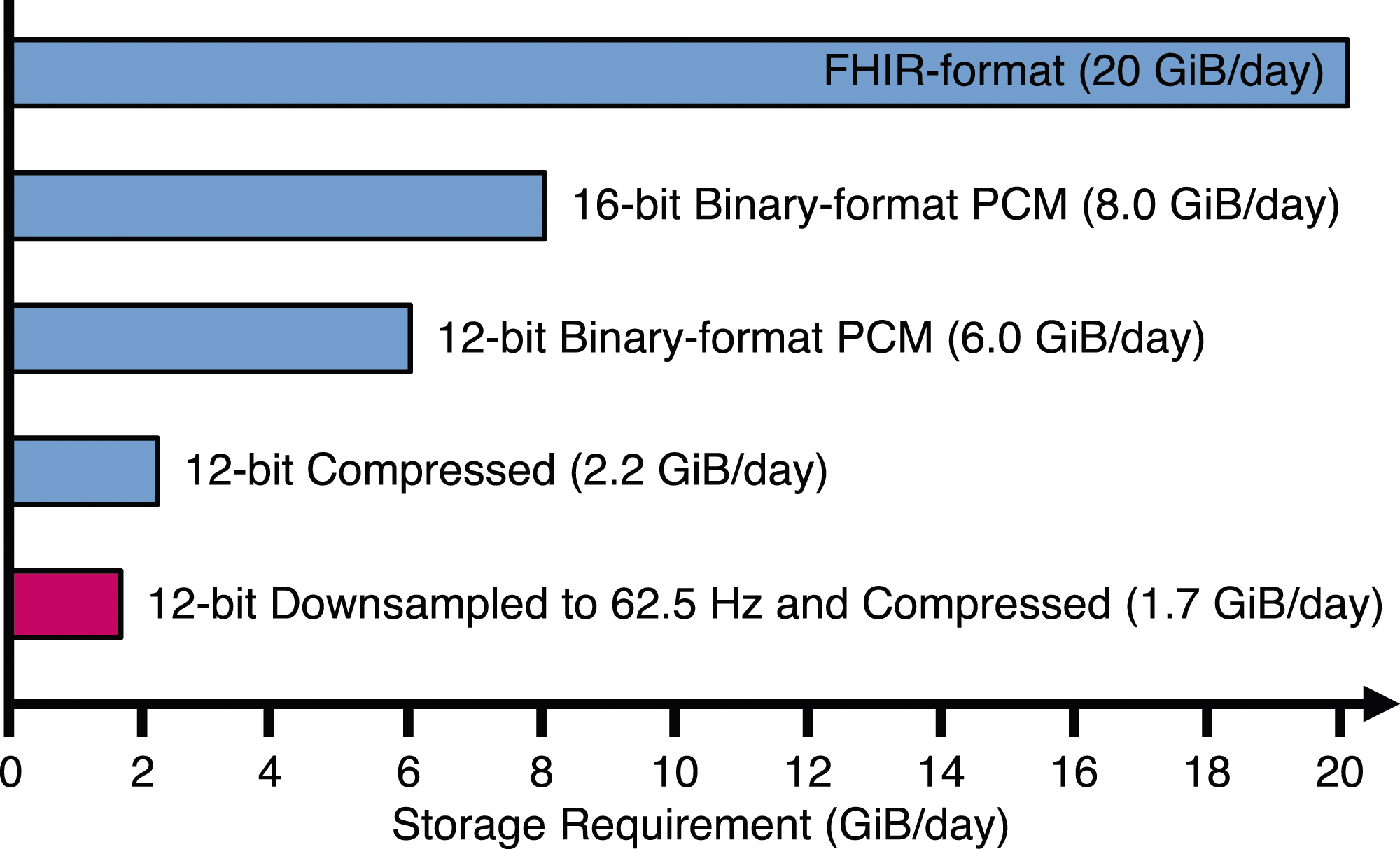

The rapid increase of health data being produced is steadily continuing and will further accelerate due to EHDS in Europe and by other similar initiatives worldwide. In summary, the main contributions of this article can be summarized as follows:

• The vast amounts of biomedical signals that need to be collected and stored, makes it important to consider compression.

• We have shown that simple lossless compression methods on typical biomedical signals does provide significant data size reduction.

• Different configurations of compression has been tested and it is clear that configurations specific to the signal type only marginally improves the compression compared to a single configuration for all types of signals.

• If a small loss is acceptable, improvements in compression ratios can be achieved by using lossy compression.

Conclusions

This article investigated the efficiency of several data compression methods on standard biomedical waveform signals generated from monitored patients. Most previous work has mainly focused on ECG signal compression, while many other biosignals are understudied. Common data format standards, such as FHIR and CSV, are inefficient for data storage. Changing to a binary representation is the first step in reducing the storage need. In this article, we proposed and investigated simple compression methods with low implementation complexity and low compression delay that can be used for many different signals and still achieve good compression ratios. It was found that Exponential-Golomb was better than Golomb-Rice, which is commonly used with ECG compression. The results indicated that it is easy to obtain compression ratios of 2.7:1 (±0.2) for arterial blood pressure curves, 2.9:1 (±0.1) for photoplethysmography, and 4.1:1 (±0.2) for respiration when using 12-bit sampling and lossless compression. We also experimented with a simple lossy compression method based on downsampling with small reconstruction errors. As part of managing an emerging avalanche of data, new simple storage strategies are needed. Many of the investigated methods allow this, which enables wide adoption.

Footnotes

Declaration of conflicting interests

The author(s) declared no potential conflicts of interest with respect to the research, authorship, and/or publication of this article.

Funding

The author(s) received no financial support for the research, authorship, and/or publication of this article.

ORCID iD

Martin Jacobsson

References

Rydning

. Worldwide idc global datasphere forecast, 2022–2026: enterprise organizations driving most of the data growth, 2022. Available at: https://www.idc.com/getdoc.jsp?containerId=US49018922

Statista . Projected health data storage limitations in 2020, 2019. Available at: https://www.statista.com/statistics/1038042/global-healthcare-data-storage-limitations/

European Commission . Proposal for a regulation - the european health data space, 2022. Available at: https://health.ec.europa.eu/publications/proposal-regulation-european-health-data-space_en

Shilo

Rossman

Segal

. Axes of a revolution: challenges and promises of big data in healthcare. Nat Med 2020; 26: 29–38. DOI: 10.1038/s41591-019-0727-5.

Ribeiro

Paixão

GMM

, et al. Automatic diagnosis of the 12-lead ECG using a deep neural network. Nat Commun 2020; 11(1760). DOI: 10.1038/s41467-020-15432-4.

Graf

Reinhold

Brunkhorst

, et al. Variability of structures in german intensive care units - a representative, nationwide analysis. Wien Klin Wochenschr 2010; 122: 572–578. DOI: 10.1007/s00508-010-1452-8.

Davies

Vistisen

Jian

, et al. Ability of an arterial waveform analysis-derived hypotension prediction index to predict future hypotensive events in surgical patients. Anesth Analg 2020; 130(2): 352–359. DOI: 10.1213/ANE.0000000000004121.

Lee

Kim

, et al. Intraoperative hypotension prediction model based on systematic feature engineering and machine learning. Sensors 2022; 22(9). DOI: 10.3390/s22093108.

van der Ster

BJP

Bennis

Delhaas

, et al. Support vector machine based monitoring of cardio-cerebrovascular reserve during simulated hemorrhage. Front Physiol 2018; 8: 1057. DOI: 10.3389/fphys.2017.01057.

10.

Tiwari

Falk

. Lossless electrocardiogram signal compression: A review of existing methods. Biomed Signal Process Control 2019; 51: 338–346. DOI: 10.1016/j.bspc.2019.03.004.

11.

Arnavut

. Ecg signal compression based on burrows-wheeler transformation and inversion ranks of linear prediction. IEEE (Inst Electr Electron Eng) Trans Biomed Eng 2007; 54(3): 410–418. DOI: 10.1109/TBME.2006.888820.

12.

Mishra

Thakkar

Modi

, et al. ECG signal compression using compressive sensing and wavelet transform. 2012 annual international conference of the IEEE engineering in medicine and biology society, 2012; 3404–3407. DOI: 10.1109/EMBC.2012.6346696.

13.

Deepu

Lian

. A joint QRS detection and data compression scheme for wearable sensors. IEEE (Inst Electr Electron Eng) Trans Biomed Eng 2015; 62(1): 165–175. DOI: 10.1109/TBME.2014.2342879.

14.

Elgendi

Mohamed

Ward

. Efficient ECG compression and QRS detection for e-health applications. Nature Scientific Reports 2017; 7: 459. DOI: 10.1038/s41598-017-00540-x.

15.

Wang

Jin

, et al. A novel lossless ecg compression algorithm for active implants. In: 2021 43rd annual international conference of the IEEE engineering in medicine biology society (EMBC), 2012; 3471–3474. DOI: 10.1109/EMBC46164.2021.9630251.

16.

Gogna

Majumdar

Ward

. Semi-supervised stacked label consistent autoencoder for reconstruction and analysis of biomedical signals. IEEE (Inst Electr Electron Eng) Trans Biomed Eng 2017; 64(9): 2196–2205. DOI: 10.1109/TBME.2016.2631620.

17.

Banerjee

Singh

. A new real-time lossless data compression algorithm for ECG and PPG signals. Preprint, 2021.

18.

Nakatsuka

Hamabe

Takeuchi

, et al. An efficient lossless data compression method based on exponential-Golomb coding for biomedical information and its implementation using ASIP technology. In: 2013 IEEE biomedical circuits and systems conference (BioCAS), 2013; 382–385. DOI: 10.1109/BioCAS.2013.6679719.

19.

Cho

Lee

. Efficient real-time lossless EMG data transmission to monitor pre-term delivery in a medical information system. Appl Sci 2017; 7(4). DOI: 10.3390/app7040366.

20.

Biagetti

Crippa

Falaschetti

, et al. Energy and performance analysis of lossless compression algorithms for wireless EMG sensors. Sensors 2021; 21: 5160. DOI: 10.3390/s21155160.

21.

Allen

Belina

. ECG data compression using the discrete cosine transform (DCT). Proceedings Computers in Cardiology, 2002; 687–690. DOI: 10.1109/CIC.1992.269340.

22.

Ranjeet

Kumar

Pandey

. ECG signal compression using different techniques. In: Advances in computing, communication and control. Springer Berlin Heidelberg, 2011; 231–241.

23.

Goodwin

Eytan

Greer

, et al. A practical approach to storage and retrieval of high-frequency physiological signals. Physiol Meas 2020; 41(3). DOI: 10.1088/1361-6579/ab7cb5.

24.

HL7. Fast healthcare interoperability resources (FIHR). Available at: http://hl7.org/fhir/

25.

Salomon

Motta

. Handbook of data compression. London: Springer-Verlag, 2010. ISBN 978-1-84882-903-9. DOI: 10.1007/978-1-84882-903-9.

26.

Goldberger

Amaral

LAN

Glass

, et al. PhysioBank, PhysioToolkit, and PhysioNet. Circulation 2000; 101(23): e215–e220. DOI: 10.1161/01.CIR.101.23.e215.

27.

Moody

Villarroel

, et al. MIMIC-III waveform database (version 1.0). Physionet, 2020. DOI: 10.13026/c2607m.

The role of compression in large scale data transfer and storage of typical biomedical signals at hospitals