Sage Journals: Discover world-class research

Abstract

Background: Increasing diabetes prevalence is a major public health concern. In this study we ask whether linked open data can be used to predict prescription volumes of drugs used in the treatment of diabetes across small geographies of England. Methods: We propose and demonstrate a methodology of utilising publicly available open data to infer the geo-spatial distribution of prescribed drugs for diabetes, at the lower layer super output area level. Multiple datasets are acquired, processed, and linked together, enabling a more in-depth analysis. Combining these linked datasets with published deprivation factors of geographies across England, we build highly predictive regression models. Results: Regression models were trained and are capable of accurately predicting diabetes prescribing volumes based on deprivation indicators of various geographies across England. Models built with data covering the city of Bradford, England, produced a predicted against actual correlation value of R² = 0.672 using multiple linear regression and 0.775 using Least Absolute Shrinkage and Selection Operator (LASSO). Median age and air quality factors proved to be significant markers for diabetes prescribing. Conclusions: The results of this study suggest our methodology is robust and accurate. Such predictive models are useful to health authorities in light of increasing costs and increasing prevalence of diabetes. While using publicly available open data negates any issues of data privacy.

Keywords

Diabetes geo-prediction open data prescribing primary care public health regression

Introduction

Diabetes prescription costs accounted for 12.5% of the total prescribing cost in England during 2018/19. The total net ingredient cost (NIC) for all prescribing across primary care was reported to be £8630 million, of which, £1075 million was accounted for by drugs and devices used to treat diabetes. In 2008/9 the NIC for antidiabetic drugs was £168 million, increasing to £540 million by 2018/19, an increase of 221.2%. Over the same period the NIC of insulins had only increased by 22.5%.¹

Studies reported in the literature have shown trends in type 2 diabetes to be increasing in childhood in the UK,² with others accounting the increasing prevalence in the older population to people living longer.³ Both contribute to an increasing national trend, which unavoidably results in an increase of diabetes drug use and rising costs to the National Health Service (NHS). Global prevalence of diabetes is estimated to rise to 10.4% by 2040.⁴

Links between the prevalence of diabetes in society and socioeconomic factors is a well established one. Trends in diabetes prescribing^5,6 as well as antibiotic prescribing^7–9 is well known to correlate with deprivation levels. Inequalities in social deprivation have been key factors in studies reporting on hospital admissions for diabetes related issues, where ethnicity and age play significant roles.⁶ Regional deprivation linked to diabetes is not only prevalent in the UK, but other countries across Europe. A study of German citizens showed deprivation contributed to a 2.4 times higher incidence of type 2 diabetes.⁵ Studies in South Korea reported similar findings, with low-income households in deprived regions having higher hospital admissions and mortality rates resulting from diabetes complications.¹⁰ Prevalence of diabetes in deprived areas suggests exposure to the factors that are involved in the causation of diabetes are more common.¹¹ Risk factors such as obesity, low physical activity, smoking, and low consumption of fresh fruit and vegetables are all more common in the most lowest socioeconomic quintile, leading at a 77% increased odds of developing diabetes than those in the highest quintiles.¹²

As diabetes prevalence can vary considerably between contiguous geographical areas,¹⁰ this study is based at the Lower Layer Super Output Area (LSOA), which is the most granular level of data available. LSOA’s are geographical hierarchies designed to facilitate statistical reporting across England, they are built from contiguous smaller geographical areas, generated automatically to be as consistent in population size as possible. An LSOA is designed to have a minimum population of 1000 and a maximum population of 3000, with a minimum household number of 400 and a maximum household number of 1200.¹³

The open data used in this study comes from publicly available official sources. Open data is typically anonymised to the extent that it rightly prevents the possibility of individuals or small groups being identified. Although the risk is not entirely eliminated, the probability of re-identification is very small.^14,15 Data sensitivity is of importance, but while anonymisation is a necessary procedure, it inevitably adds an element of noise to the data, which is difficult to quantify. Furthermore when using multiple sets of open data, the error is amplified and modelling of such data can prove challenging. Here, concepts of linked open data are utilised in an attempt to overcome the granularity issues that are inherent with open data.

In this study we propose a methodology using linked open data to predict diabetes prescription volumes for geographical locations across the local authority district (LAD) of Bradford (city of), based in the county of West Yorkshire. Six different datasets are combined to infer regression models that can approximate levels of diabetes prescription volumes by geography. To keep the analysis manageable, we report findings for the city of Bradford, but similar analysis can be applied to other cities across the country. Bradford is of particular interest, since the prevalence of diabetes is much higher in the city’s population compared to the national average,¹⁶ a trend accounted to a more steeply rising incidence seen in the South Asian demographic of the city.¹⁷

An NHS commissioned study of the Bradford Clinical Commisioning Group (CCG) demonstrated that for diabetes and other endocrine nutritional and metabolic problems, there were substantial opportunites for improvments in quality, outcomes and prescribing expenditure. Savings in excess of £1.85 million were estimated to be achievable.¹⁸

The motivation behind this study is therefore driven by two aims; (1) to help reduce, plan or foresee costs for health authorities in their efforts to tackle diabetes from a financial perspective and (2) to discern the usefulness of publicly available open data to build predictive prescribing models.

A predictive model for prescription volumes is a useful tool for health authorities as well as local authorities to manage and foresee future costs and trends. The knowledge gained from such analysis could help inform decisions and services offered to populations within small geographical areas (LSOA areas have a maximum population of 3000) to help manage escalating diabetes prevalence.

Using artificial intelligence in medical AI applications is an active area of discussion. Proposed frameworks are being formalised to help manage human rights and privacy protection concerns.¹⁹ The work proposed in this study utilises publicly available open data and therefore negates data privacy issues, while using concepts of linked data, enables a wider scope of analysis to be performed.

Related work reported in the literature mainly focuses on time trend and geographical variations in diabetes.²⁰ Where predictive prescribing cost models are concerned, more dated work was found, which looked at total prescribing costs at the GP practice level using predominately patient age demographics.^21,22 A predictive prescribing model using linked open data, aimed at small geographies across England is not currently available in the literature.

Method

Data

All the data used in this study come from open publicly available resources, and are readily available online following the links provided (Table 1). To avoid the pitfalls of irregular or inflated prescribing as seen during the Covid-19 pandemic period,²³ this study uses data from the pre-pandemic period of 2019 where possible.

Table 1.

List of data resources used in this study.

Data	Source	Ref
English prescribing data (Jan’19–Dec’19)	NHSBSA	24
National statistics postcode lookup (Nov’19)	ONS open geography portal	25
LSOA to wards (2019)	ONS open geography portal	26
Patients registered at a GP practice (Oct’19)	NHS digital	27
LSOA population estimates (Mid-2019)	ONS	28
Indices of multiple deprivation 2019 (file 7)	GOV.UK	29

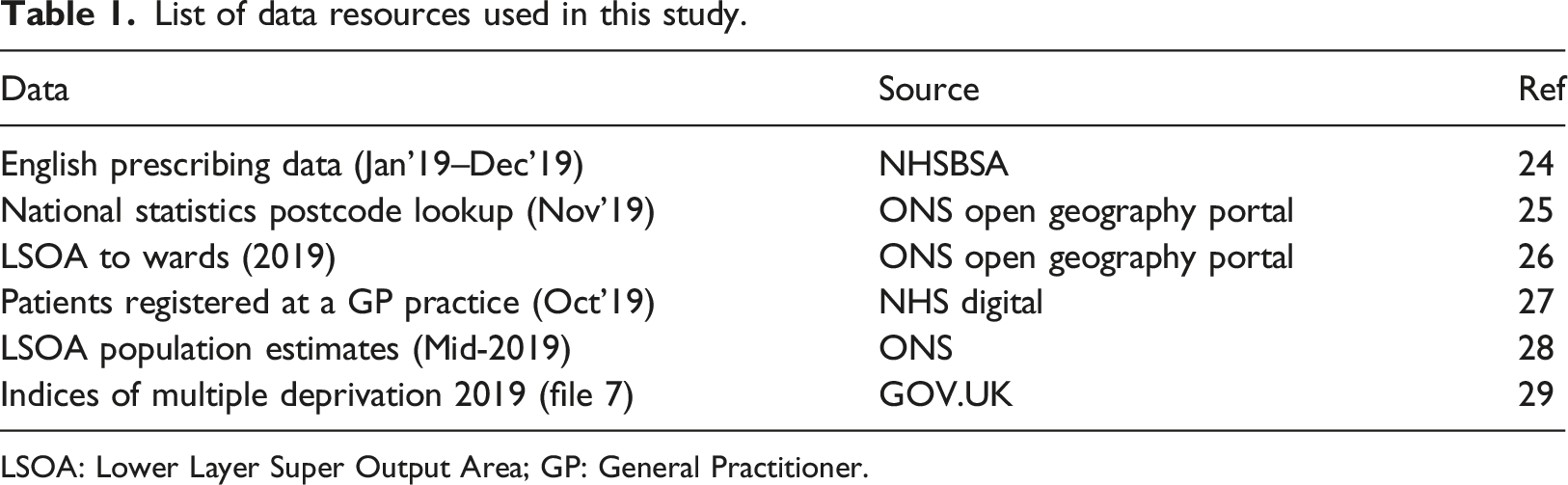
LSOA: Lower Layer Super Output Area; GP: General Practitioner.

EPD data

The first data acquired was the English prescribing data (EPD),²⁴ for the months of Jan 2019–Dec 2019. The EPD contains information regarding all prescriptions issued in England. The data records “items”, which refers to an instance of a drug type, appliance, dressing or reagent requested by a prescription form. No individual patient identifiable information is available.²⁴ For this study the useful features in the data were the items, the total quantity, the address of the General Practitioner (GP), the unique code assigned to the GP (Practice code) and the drug prescribed. The drug prescribed is listed with it’s British National Formulary (BNF) code and BNF description.³⁰ The BNF code is a 15 character code used by the NHS to classify drugs and preparations. This code can be used to filter groups or classes of drugs used for the treatment of a particular condition. Other features such as net ingredient cost (NIC) and total cost have been used in studies reporting the increasing cost of prescription medicines in England.^1,23 The EPD is a monthly release of all prescriptions dispensed, each file contains in the region of 17–18 million records, resulting in a combined total of approximately 214 million records for the year of 2019.

National statistics postcode lookup data

To identify which LSOA boundary a particular GP practice from the EPD dataset is located, a postcode to LSOA lookup file was required. For statistical and geographical consistency the Office for National Statistics (ONS) recommends the use of the National Statistics Postcode Lookup (NSPL).²⁵ For this study the Nov 2019 version was used, and contained approximately 2.6 million records. The NSPL contains information regarding the date of a postcode’s introduction as well as termination if the postcode no longer exists. Geo-coordinate information in the form of latitude and longitude records are available as well as geo-mapping information allowing postcodes to be mapped to their relevant LSOA geographical region.

LSOA to wards data

To filter data for the desired LAD (city of Bradford), a lookup file which mapped LSOAs to LADs was used. The LSOA to Ward file which mapped LSOAs of 2011 to Wards of 2019 was obtained from the ONS Open Geography Portal website.²⁶ While this file is labelled as an LSOA to Ward lookup, it also contains LAD lookup information. The data in this file is therefore used to identify the LSOA regions which map to the LAD of interest (i.e., city of Bradford). There are 34,753 records in the dataset covering all LSOA regions of the UK.

Patients registered at a GP practice data

Quantities of diabetic drugs prescribed by a particular GP can be obtained from the EPD dataset, but it must be mapped to LSOA geographies to understand which areas have a higher prevalence of diabetes medications. A file containing the Patients Registered at a GP Practice was obtained from the NHS Digital website.²⁷ This is a monthly release, however, every quarterly publication also includes the number of patients registered at a GP by LSOA region. The Oct 2019 version was used in this study. This file contained approximately 814,000 records, with features including the name of the GP practice, a unique practice code, together with the number of patients registered per LSOA region.

LSOA population estimates data

LSOA regions are defined by their population and household numbers, but the differences in population between LSOA regions can differ significantly. When summing prescription totals per LSOA region, we must adjust for the population of the LSOA region. The mid-year lower layer super output area population estimates file was obtained from the ONS website,²⁸ it contains population estimates by single year of age for all LSOA regions in England and Wales. The file can be linked to other datasets via the “Area Codes” (LSOA code) field. The Mid-2019 dataset was chosen for this study, it contains 34,753 records, covering all LSOA regions of the UK.

Indices of multiple deprivation data

As diabetes has an established correlation with social deprivation, the final dataset required for this study was the English indices of deprivation 2019 (IoD2019) data.²⁹ This file provides a measure of relative deprivation for the 32,844 LSOA regions of England. Seven different domains or facets of deprivation are reported; (1) Income deprivation, (2) Employment deprivation, (3) Education, skills and training deprivation, (4) Health deprivation and disability, (5) Crime, (6) Barriers to housing and services, and (7) Living environment deprivation. The seven domains are combined into a single “Index of multiple deprivation” (IMD) using a weighting system devised from academic literature and robustness of the indicators.²⁹ Deprivation scores are turned into ranks whereby rank 1 is the most deprived and rank 32,844 is the least deprived region in England. Alongside ranks, deprivation deciles are reported which categorise regions into 10 equal groups with decile 1 being the most deprived regions and decile 10 being the least deprived regions. In this study, “File 7” as named at the source²⁹ was used. File 7 contains all the scores, ranks and deciles of the LSOA regions compiled into a single file.

Data processing

The R statistical programming language³¹ was used to mine and analyse all the data in this study. To begin, all 12 EPD files were combined into one large file. Using the 15 character BNF code feature of the dataset, the data were filtered for drugs used in the treatment of diabetes. This included insulin, antidiabetic drugs (e.g., metformin) and drugs used to treat hypoglycaemia (e.g., glucagon). It did not include diabetic diagnostic and monitoring devices which are also prescribed on the NHS and available in the dataset.

To identify which prescribing GPs were based within the desired local authority district of Bradford, two further files were required. Firstly, the NSPL dataset was used, which allowed the postcode of each GP to be mapped to an LSOA code and therefore an LSOA region in the country. Next, the LSOA code, was used to map to higher geographies using the LSOA to Ward lookup file. This allowed LSOAs to be mapped to wards and subsequently to the relevant LAD regions. The EPD data can therefore be filtered for the desired GPs which reside in the LAD of interest together with the total number of diabetes items these GP’s prescribed.

As this study attempts to map and predict prescription volumes at the geographical LSOA level, it must be determined which LSOA region a GP’s prescribed medicine is going to, i.e., which geographical location (LSOA) does the patient who was prescribed a medicine live in. In actuality this cannot be determined from the open data available. However in this study we postulate using a GP’s patient list size data to approximate the ratio of medicines being prescribed to each LSOA region.

For example, Figure 1 shows the patient demographic of GP practice B83005 (practice code). This GP resides in the local authority of Bradford, and has a total patient list size of 6885. Using the Patients Registered at a GP Practice dataset (see Table 1), which contains information on the total number of patients per GP residing in any given LSOA region, we can graphically visualise the patient demographic distribution for GP B83005, as shown in Figure 1. The figure shows a heat map, ranging from red (high) to yellow (low), of the patient numbers residing in specific LSOA regions.

Figure 1.

Patient demographic of GP practice code B83005 at the LSOA level.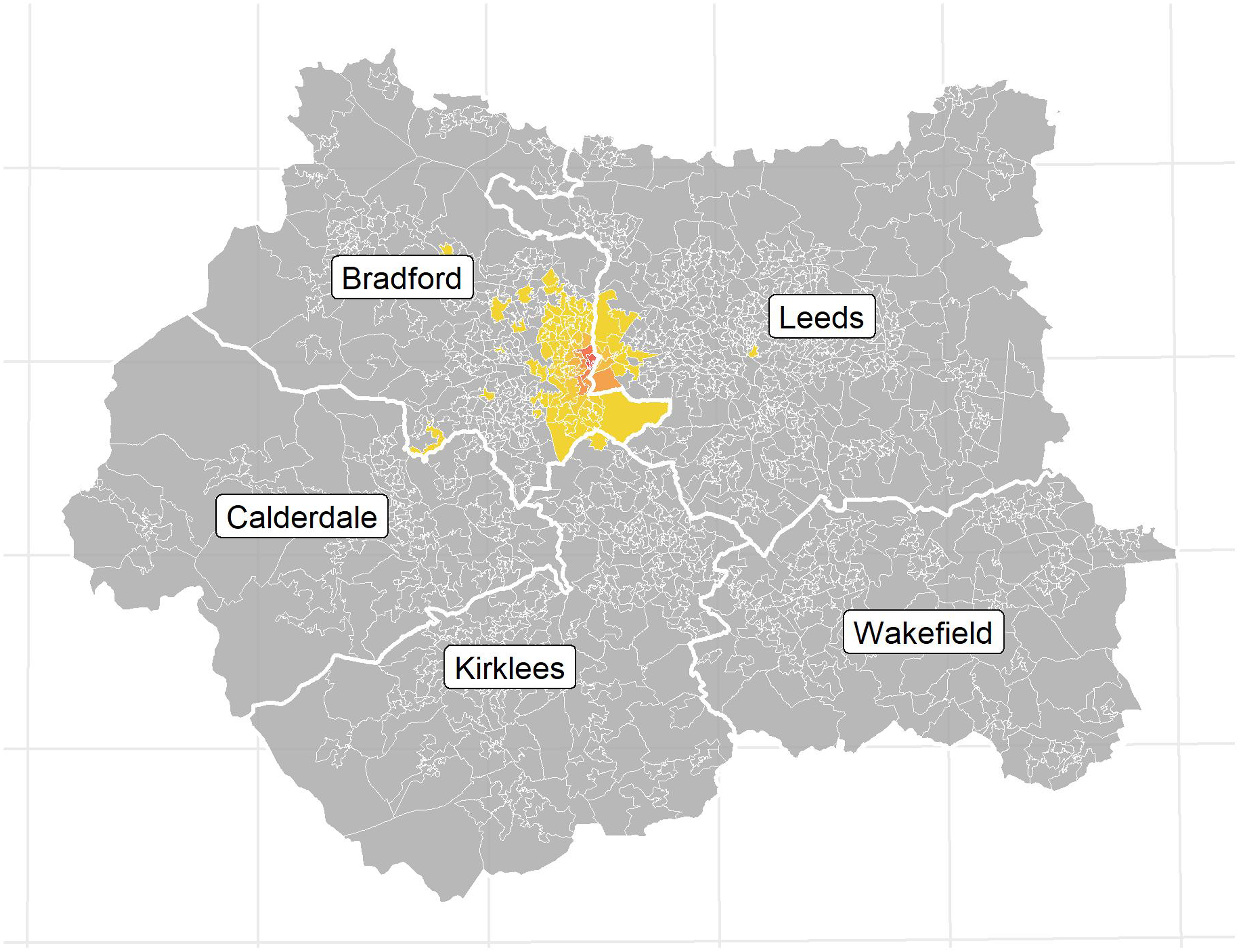

Using the demographic distribution for every GP practice of interest, we then calculate the distribution of the diabetes drugs prescribed. An excerpt for GP B83005 is shown in Table 2. The table shows a list of the LSOA regions that GP B83005 serves, and how many patients reside in each region. Using this information two further metrics, % patients and weighted items (wt_items), are calculated as follows:

% p a t i e n t s = \frac{N o . o f p a t i e n t s i n L S O A}{T o t a l p a t i e n t s r e g i s t e r e d a t G P} \times 100

(1)

w t_i t e m s = \frac{% p a t i e n t s}{100} \times t o t a l i t e m s

(2)

Table 2.

Excerpt data of GP Practice code B83005, with total patient population of 6885 and total diabetes prescribed item sum of 6865.

LSOA	No. of patients	% Patients	wt_items
E01010612	46	0.668	45.866
E01010613	15	0.218	14.956
E01010614	52	0.755	51.849
E01010615	1	0.015	0.977
E01010616	1	0.015	0.977
E01010617	21	0.305	20.939
E01010618	791	11.489	788.702
E01010619	478	6.943	476.611

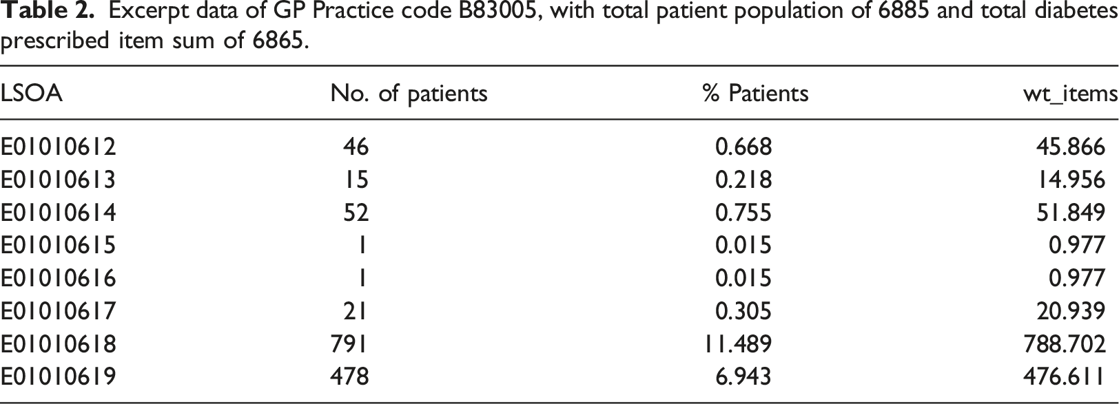
Note, the ‘Total Patients registered at GP’ is derived from the Patients Registered at a GP Practice dataset, and the ‘Total items’ is the total number of diabetes items prescribed by a GP and is derived from the EPD dataset (Table 1). For GP B83005 the total items prescribed was 6865.

Since an LSOA region can and will be served by more than one GP, it is necessary to find all GPs that serve a given LSOA and sum all the wt_items values for that region. Doing this for all GPs in the study, results in the total sum of wt_items (LSOA total) for every LSOA for which data are available.

Consider all LSOAs available in the study to be represented by the array LSOA = [LSOA_i…LSOA_n], then;

L S O A_{i} t o t a l = \sum_{G P = 1}^{n} L S O A_{i} w t_i t e m s

(3)

Although LSOA regions have set minimum and maximum values for population and households, the differences can be influential in such analysis. Consequently the LSOA total is adjusted for by population. To achieve this we use the LSOA population estimates dataset from the ONS (Table 1). This file contains mid-year population estimates for every LSOA region in the country. Using the LSOA population estimate, the adjusted total (adj_total) is calculated as follows:

a d j_t o t a l = \frac{L S O A_{i} t o t a l}{P o p u l a t i o n o f L S O A_{i}} \times 100

(4)

For regression analysis (see below), the adj_total becomes the dependent variable in the study. For the independent variables the indices of deprivation dataset (File 7) is used (see Table 1). This file contains deprivation scores, ranks and deciles for every LSOA region in the country. LSOA regions that fall within the LAD of this study were filtered for and only the deprivation scores from the dataset used as the independent variables. Scores consisted of additional indicators to the seven main deprivation indicators. In total, 15 score indicators were initially considered together with the median age of the LSOA region calculated from the LSOA population estimates dataset, making 16 independent variables in total. The adj_total value for each LSOA of interest was therefore matched to the relevant independent variables by LSOA code prior to regression analysis.

Regression model analysis

After processing, and prior to regression model analysis our dataset consisted of 310 records and 17 features, 16 independent variables and 1 dependent variable (see Table 3). For this study, two approaches to regression analysis are employed. The first uses multiple linear regression³² addressing multicollinearity prior to model training. The second approach employs regularization and a variant of linear regression known as LASSO (Least Absolute Shrinkage and Selection Operator).³³ Since all variables were of numerical form (continuous data), regression analysis was preferred as it allows multiple independent variables to be regressed against the dependent variable. The goal of the two approaches chosen is to aid with model interpretability and overcome issues of overfitting.

Table 3.

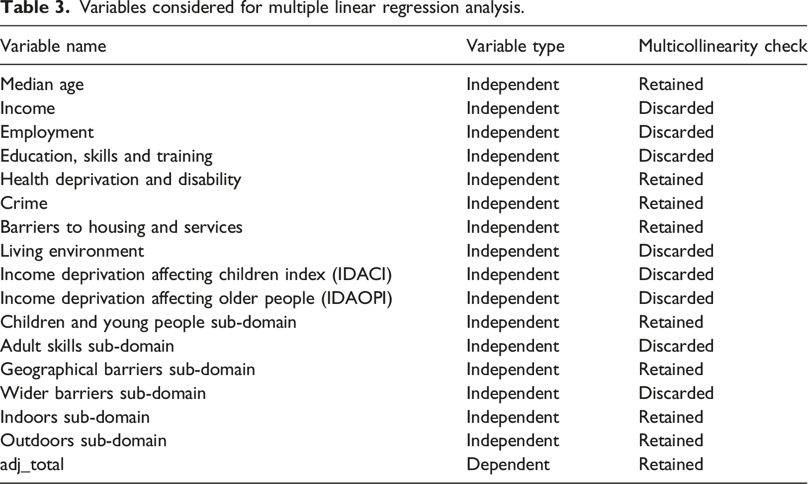
Variables considered for multiple linear regression analysis.

Variable name	Variable type	Multicollinearity check
Median age	Independent	Retained
Income	Independent	Discarded
Employment	Independent	Discarded
Education, skills and training	Independent	Discarded
Health deprivation and disability	Independent	Retained
Crime	Independent	Retained
Barriers to housing and services	Independent	Retained
Living environment	Independent	Discarded
Income deprivation affecting children index (IDACI)	Independent	Discarded
Income deprivation affecting older people (IDAOPI)	Independent	Discarded
Children and young people sub-domain	Independent	Retained
Adult skills sub-domain	Independent	Discarded
Geographical barriers sub-domain	Independent	Retained
Wider barriers sub-domain	Independent	Discarded
Indoors sub-domain	Independent	Retained
Outdoors sub-domain	Independent	Retained
adj_total	Dependent	Retained

Multiple linear regression

Prior to multiple linear regression analysis, independent variables must be assessed for multicollinearity which can be problematic if model interpretability is necessary. An assessment of the multicollinearity between the independent variables was tested by calculating the variance inflation factor (VIF). Multicollinearity exists when there is correlation between two or more independent variables. Although the accuracy of a model may not be affected much, in the presence of multicollinearity the interpretability of a regression model becomes difficult. The VIF score of an independent variable attempts to explain how well that variable is explained by the other independent variables. Where multicollinearity exists, it is important to remove those variables, since the information it provides with respect to the dependent variable is redundant when the other independent variables are present.^34,35 The minimum VIF score is 1, which indicates no correlation. There is no upper limit to a VIF score. A VIF score greater than 5 suggests the variable should be removed from the independent variables pool.³⁵

For this study a backward elimination process to remove collinear variables was employed. The VIF is calculated across all independent variables and the variable with the highest VIF score is filtered out. The process repeats until all remaining variables are below the VIF threshold of 5. This process removed eight of the independent variables which were deemed to be redundant to the analysis. Nine variables (eight independent and one dependent) were retained and used as part of the multiple linear regression analysis (see Table 3).

A multiple linear regression learner was then used to train a model, based on a random 70:30 training:test split of the data. All variables (dependent and independent variables) in both the training set and testing set were independently normalised using Z-score normalisation, which transforms values of each feature into a Gaussian distribution, with mean of 0.0 and standard deviation of 1.0. The adj_item variable was set as the target value with the 8 retained score indicators used to regress against (see Table 3). To test the robustness of the data, 500 iterations of the multiple linear regression model were trained and tested. For each iteration a new random 70:30 training:test split was used.

LASSO regression

LASSO regression is a variant of multiple linear regression that utilises regularization for feature selection and attempts to avoid issues of overfitting and multicollinearity. It does this by introducing a “penalty” to the best fit derived from the trained data, to achieve a lower variance from the test data. LASSO lessens or eliminates the influence of independent variables it deems redundant in a process known as shrinkage. LASSO encourages simple and sparse models and is an attractive option where high multicollinearilty exists or automated feature selection/reduction is a requirement.

For this study LASSO regression was used with all 16 independent variables, allowing the model to shrink or remove variables it considers redundant. A lambda parameter can be set to control the amount of shrinkage of the variables. The higher the lambda value, the more the coefficients of the variables are shrunk towards zero. A lambda search option was employed to automatically find the optimal lambda value using a heuristic based on the training data. The resulting model is based on the best found lambda value.

A LASSO regression learner was used to train a model, based on a random 70:30 training:test split of the data. All variables (dependent and independent variables) in both the training set and testing set were independently normalised using Z-score normalisation. Since LASSO introduces a penalty which affects the coefficients, differences in scaling may result in differences in the choice of optimal coefficients. The adj_item variable was set as the target value with all 16 independent variables used to regress against. 500 iterations of the LASSO regression model were trained and tested. For each iteration a new random 70:30 training:test split was used.

Results

Multiple linear regression model

The performance and coefficients outcome of the final iteration of the multiple linear regression model is presented in Table 4. Of the eight independent variables used in training, four variables produced a small p-value. A small p-value (Pr (

> | t | \leq

0.05) suggests those independent variables are unlikely to produce a relationship with the dependent variable by chance, i.e. those variables have a statistically significant affect on the dependent variable. The variables which produced a p-value of ≤0.05 are; Medain age, Health Deprivation and Disability, Indoors Sub domain and Outdoors Sub domain. The overall model p-value is also shown to be below the 0.05 significance level (<2.2 × 10⁻¹⁶). The R-squared and Adjusted R-squared for the model were 0.6933 and 0.6815 respectively.

Table 4.

Multiple linear regression model results (final iteration) (**(Pr ( $> | t | \leq$ 0.001), *(Pr ( $> | t | \leq$ 0.05)).

	Coefficients	Std.Error	t-value	Pr $(> \| t \|)$
(Intercept)	−1.220 × 10⁻¹⁵	3.831 × 10⁻²	0.000	1.000
Median age	−5.203 × 10⁻¹	7.625 × 10⁻²	−6.824	9.50 × 10⁻¹¹ **
Health deprivation and disability score	1.665 × 10⁻¹	7.400 × 10⁻²	2.250	0.0255 *
Crime	−9.211 × 10⁻²	6.756 × 10⁻²	−1.363	0.1742
Barriers to housing and services	2.462 × 10⁻²	6.447 × 10⁻²	0.382	0.7030
Children and young people sub domain	−1.067 × 10⁻¹	7.905 × 10⁻²	−1.349	0.1787
Geographical barriers sub domain	5.126 × 10⁻²	7.821 × 10⁻²	0.655	0.5129
Indoors sub domain	9.253 × 10⁻²	4.581 × 10⁻²	2.020	0.0446 *
Outdoors sub domain	3.775 × 10⁻¹	6.182 × 10⁻²	6.106	4.93 × 10⁻⁹ **

Residuals
Min	1Q	Median	3Q	Max
−2.5361	−0.3154	0.0007	0.3055	1.7912
Residual standard error: 0.5644 on 208 degrees of freedom
Multiple R-squared: 0.6933, adjusted R-squared: 0.6815
F-statistic: 58.76 on 8 and 208 DF, p-value: $<$ 2.2 × 10⁻¹⁶

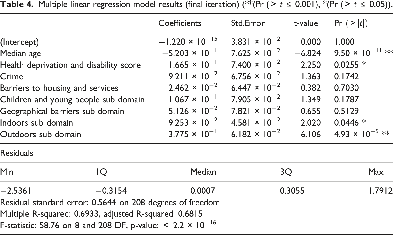
The predictive power of a model is evaluated by running the test set against the trained model to assess the fit of the model. The residuals (actual - predicted) can be examined to understand if there are any nonlinear relationships, major outliers or heteroscedasticity.

Figure 2 graphically depicts the performance of the final iteration of the multiple linear regression model, a correlation of R² = 0.689 is observed (Plot A) when the predicted values are plotted against actual, suggesting the model has good predictive accuracy. Residuals of the model were calculated and normalised (Z-score). A scatter plot and histogram of the residuals is shown in Figure 2 (Plot B and C). The scatter plot (Plot B), which plots standardised residuals against predicted values, shows the residuals are symmetrically distributed with no obvious indication of heteroscedasticity, outliers or nonlinear relationships. The histogram (Plot C) shows the distribution of model residuals to be normally distributed, i.e., the model predicts above and below the actual value evenly with no obvious bias.

Figure 2.

Graphical visualisation of the final iteration of the multiple linear regression model test set. Predicted against actual (A), Standardised Residuals against Predicted (B), and Histogram of residuals (C).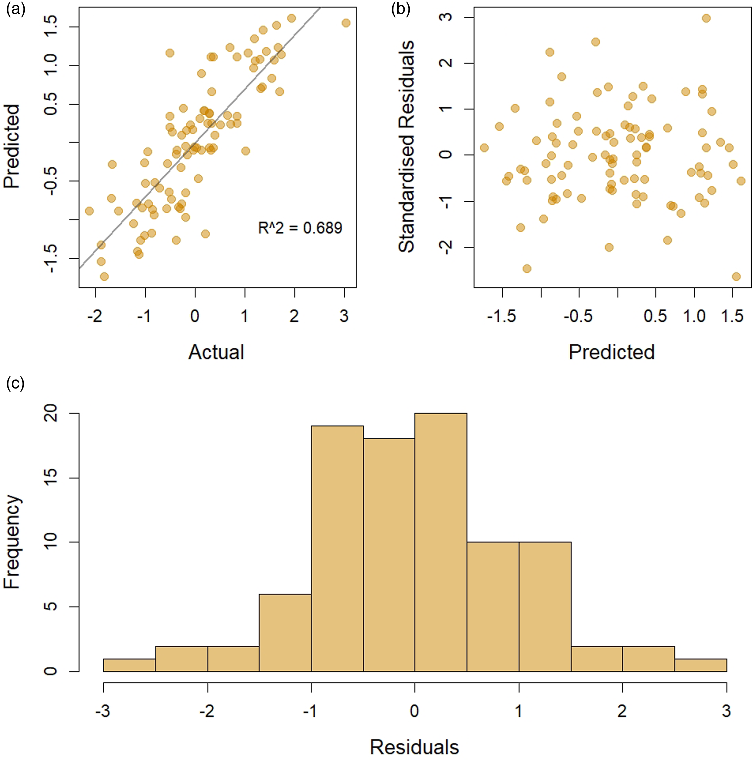

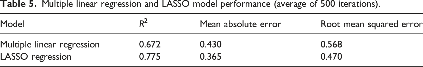
Data from the final iteration of the multiple linear regression model (see Table 4) illustrates a typical example. A summary of the 500 iterations is presented below. Table 5 records the predictive performance of the models tested, reporting the average values across all 500 iterations for R², the mean absolute error (MAE) and the root mean squared error (RMSE) values. The minimum R² value produced was 0.503 while the maximum R² value was 0.804, with a mean of the 500 iterations resulting in an R² value of 0.672. Figure 3 shows the distribution of the R² values for each linear regression model plotted as a boxplot (A) and histogram (B), a noticeable left skew is present in the distribution, suggesting more models than not of the 500 iterations produced good predictive models (i.e., higher R² values).

Table 5.

Multiple linear regression and LASSO model performance (average of 500 iterations).

Model	R ²	Mean absolute error	Root mean squared error
Multiple linear regression	0.672	0.430	0.568
LASSO regression	0.775	0.365	0.470

Figure 3.

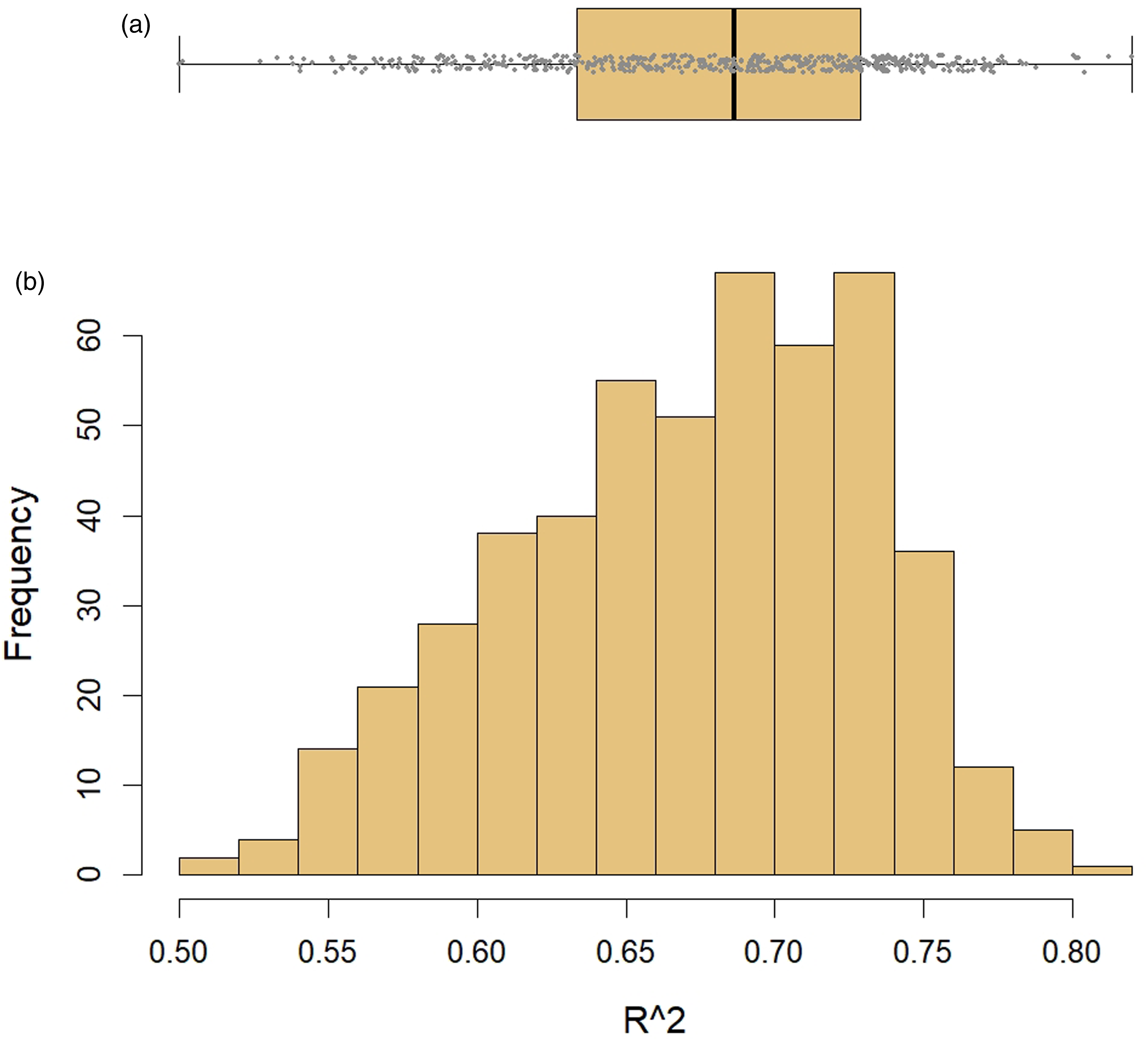
R² results of all 500 iterations of the multiple linear regression models, represented as a boxplot (A) and histogram (B), producing a mean R² of 0.672 with standard deviation of 0.059.

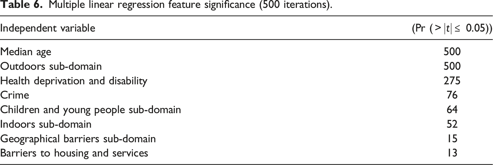
To understand the influence of the independent variables during training of the multiple linear regression models, an assessment of the variables resulting in p-values of ≤0.05 were extracted and are shown in Table 6. For all 500 iterations, two variables; Median age and Outdoors Sub-domain resulted in p-values of ≤0.05, and are considered statistically significant in all the multiple linear regression models produced. Health Deprivation and Disability resulted in a p-value of ≤0.05 for 275 of the 500 models trained. All other independent variables resulted in p-values of ≤0.05 for approximately 15% or less of the 500 trained models (see Table 6).

Table 6.

Multiple linear regression feature significance (500 iterations).

Independent variable	(Pr ( $> \| t \| \leq$ 0.05))
Median age	500
Outdoors sub-domain	500
Health deprivation and disability	275
Crime	76
Children and young people sub-domain	64
Indoors sub-domain	52
Geographical barriers sub-domain	15
Barriers to housing and services	13

LASSO regression models

LASSO regression models were used in this study as an alternative approach to handle multicollinearity and perhaps aid with model interpretability. It is of particular interest to check if the penalty function of LASSO regression produces sparse models that corroborate in variable selection/significance to the multiple linear regression models.

The coefficient outcome of the final iteration of the LASSO regression model is shown in Table 7. Five independent variables (Income, Employment, Living Environment, Geographical Barriers Sub-domain, and Wider Barriers Sub-domain) have had their coefficients reduced to zero, and are therefore completely removed from the model. These variables were considered not to have any influence on the dependent variable. Of the remaining independent variables several have resulted in small coefficients, e.g., Crime (−0.005), see Table 7. Only four variables, Adult Skills Sub-domain, Outdoors Sub-domain, Median age, and Education, Skills and Training, resulted in an absolute coefficient value of ≥0.1. Interestingly, two of these independent variables, Median age and Outdoors Sub-domain, were also statistically significant in all 500 iterations of the multiple linear regression models (see Table 6).

Table 7.

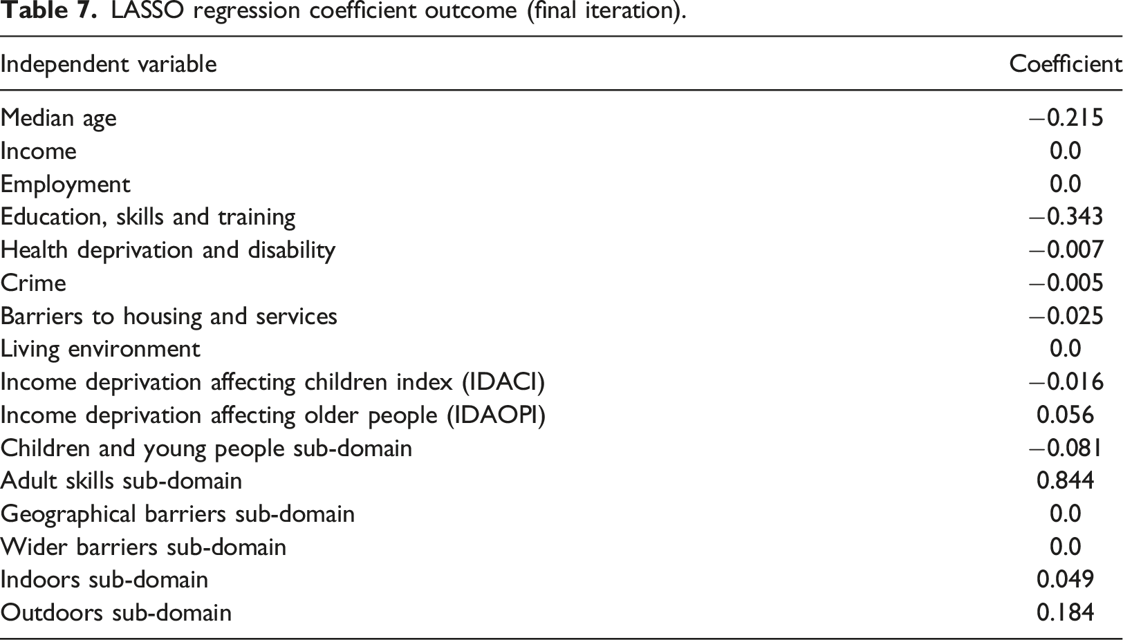
LASSO regression coefficient outcome (final iteration).

Independent variable	Coefficient
Median age	−0.215
Income	0.0
Employment	0.0
Education, skills and training	−0.343
Health deprivation and disability	−0.007
Crime	−0.005
Barriers to housing and services	−0.025
Living environment	0.0
Income deprivation affecting children index (IDACI)	−0.016
Income deprivation affecting older people (IDAOPI)	0.056
Children and young people sub-domain	−0.081
Adult skills sub-domain	0.844
Geographical barriers sub-domain	0.0
Wider barriers sub-domain	0.0
Indoors sub-domain	0.049
Outdoors sub-domain	0.184

For a selection of independent variables that are highly correlated amongst themselves, LASSO tends to pick one randomly and shrink the others to zero, which effectively removes their influence from the model. While the variance inflation factor used prior to multiple linear regression removed the independent variables Adult Skills Sub-domain and Education, Skills and Training, LASSO retained these variables, using Adult Skills Sub-domain in all 500 iterations and Education, Skills and Training in 409 of the 500 iterations. Table 8 summarises the number of times (of 500 iterations) an independent variable’s coefficient was ≠ 0.

Table 8.

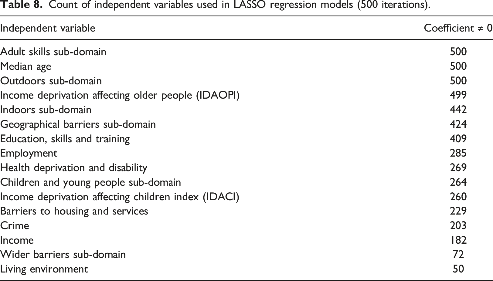
Count of independent variables used in LASSO regression models (500 iterations).

Independent variable	Coefficient ≠ 0
Adult skills sub-domain	500
Median age	500
Outdoors sub-domain	500
Income deprivation affecting older people (IDAOPI)	499
Indoors sub-domain	442
Geographical barriers sub-domain	424
Education, skills and training	409
Employment	285
Health deprivation and disability	269
Children and young people sub-domain	264
Income deprivation affecting children index (IDACI)	260
Barriers to housing and services	229
Crime	203
Income	182
Wider barriers sub-domain	72
Living environment	50

The predictive capabilities of the LASSO regression models were evaluated by running the test sets against the trained models to asses the fit of the models for each iteration. Figure 4 graphically depicts the performance of the final iteration of the LASSO regression model. A correlation of R² = 0.753 is observed (Plot A) when the predicted values are plotted against the observed, suggesting the model has good predictive accuracy, and is a significant improvement on the multiple linear regression models. A scatter plot and histogram (Plot B and C) of the normalised residuals show the residuals to be symmetrically distributed with no clear indication of heteroscedasticity, outliers or nonlinear relationships. The histogram shows a normal distribution of the residuals suggesting the model does not have an obvious bias in its predictions.

Figure 4.

Graphical visualisation of the final iteration of the LASSO regression model test set. Predicted against actual (A), Standardised Residuals against Predicted (B), and Histogram of residuals (C).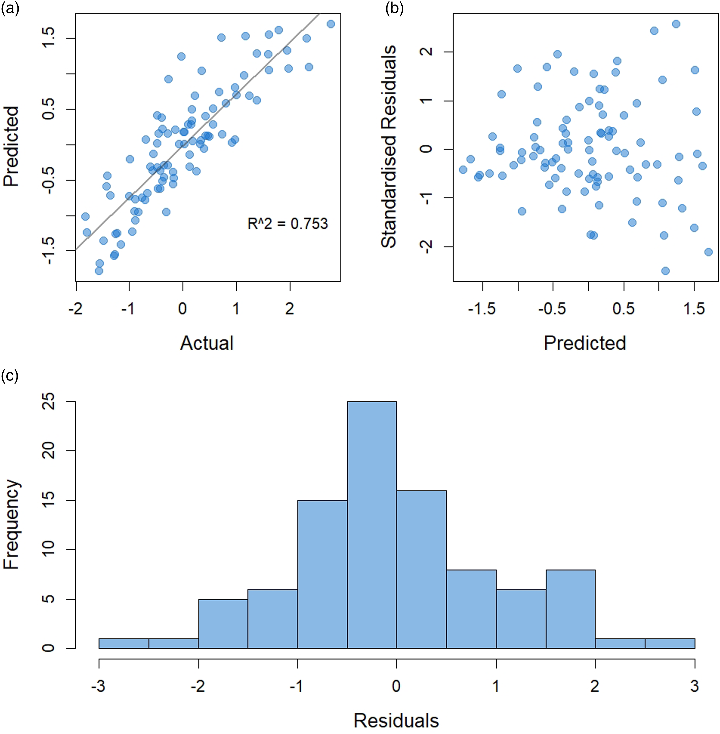

A summary of the 500 iterations of the LASSO models are presented in Table 5. A mean R² value of 0.775 is observed for the 500 iterations, with a minimum R² value of 0.644 and a maximum of 0.870. The mean absolute error (0.365) and root mean squared error (0.470) were both lower than that for the multiple linear regression models, suggesting we have more accurate models with LASSO regression. Figure 5 shows the distribution of the R² values for each LASSO regression model plotted as a boxplot (A) and histogram (B). As with the multiple linear regression models, a left skew is observed, suggesting many of the iterations resulted in good predictive models.

Figure 5.

R² results of all 500 iterations of the LASSO regression models, represented as a boxplot (A) and histogram (B), producing a mean R² of 0.775 with standard deviation of 0.041.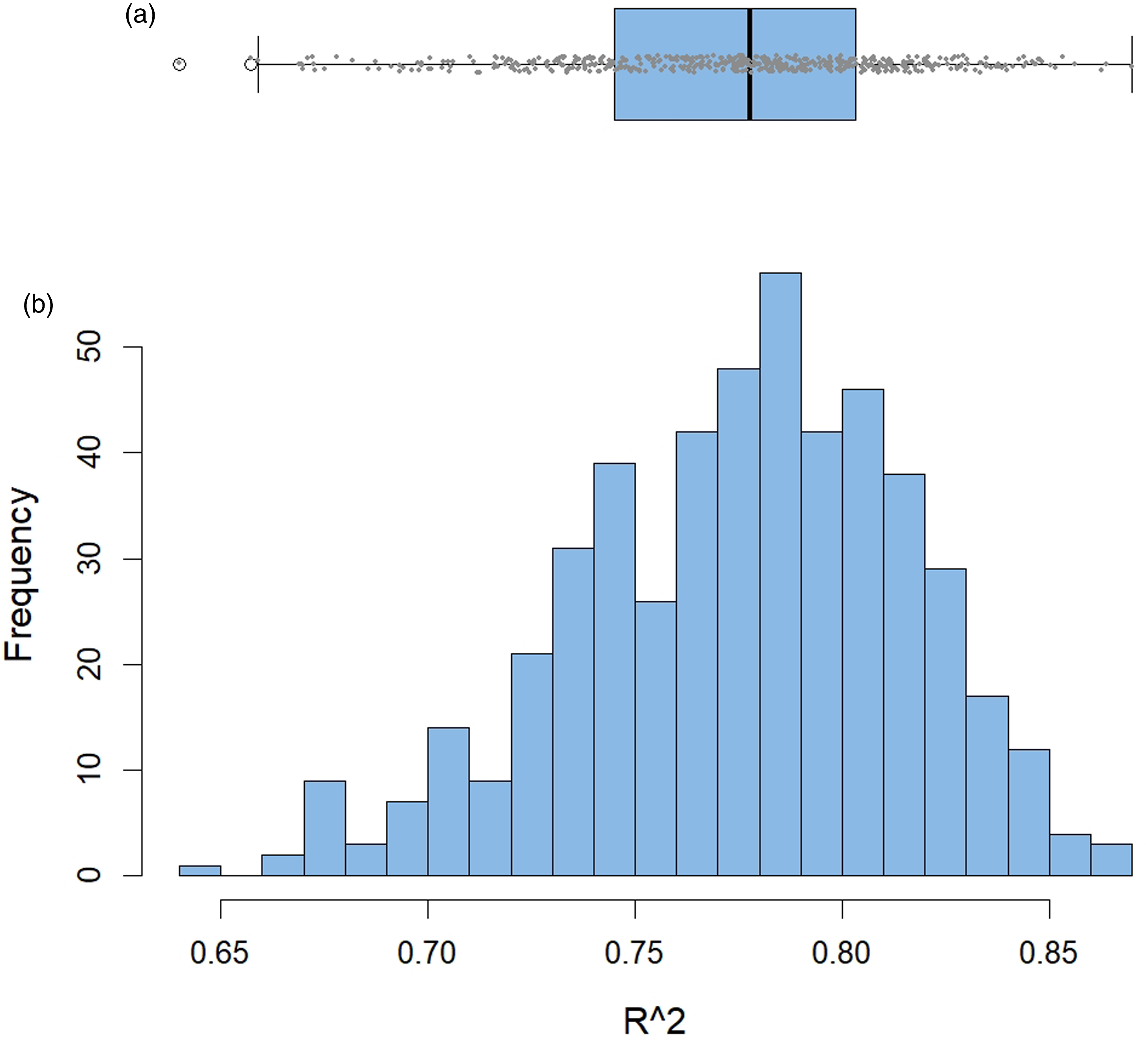

Since LASSO coefficients are penalised according to feature importance it is more relevant to assess which features were reduced to zero (or a very small value) and which features where consistently retained by the LASSO models. Figure 6 shows the mean coefficient values calculated from all 500 iterations of the LASSO regression models, for each of the 16 independent variables used. To illustrate feature importance an arbitrary coefficient value of ±0.1 was chosen, based on the coefficient outcome of the last iteration of the LASSO models (see Table 7). Across 500 iterations of the LASSO regression models, 5 independent variables produced a mean coefficient value of −0.1 ≤ x ≥ 0.1. These variables are, Outdoors Sub-domain, Median age, Income Deprivation Affecting Older People (IDAOPI), Education, Skills and Training, and Adult Skills Sub-domain. Four of these variables, Outdoors Sub-domain, Median age, Education, Skills and Training, and Adult Skills Sub-domain, match the results of the final iteration of the LASSO models (see Table 7). Two of these variables, Outdoors Sub-domain, and Median age, were also statistically significant in the multiple linear regression models, suggesting some corroboration of feature importance between the two methods used.

Figure 6.

Mean coefficient value of all 16 independent variables across 500 iterations of the LASSO regression model. The red dashed line shows an arbitrary coefficient value of ±0.1.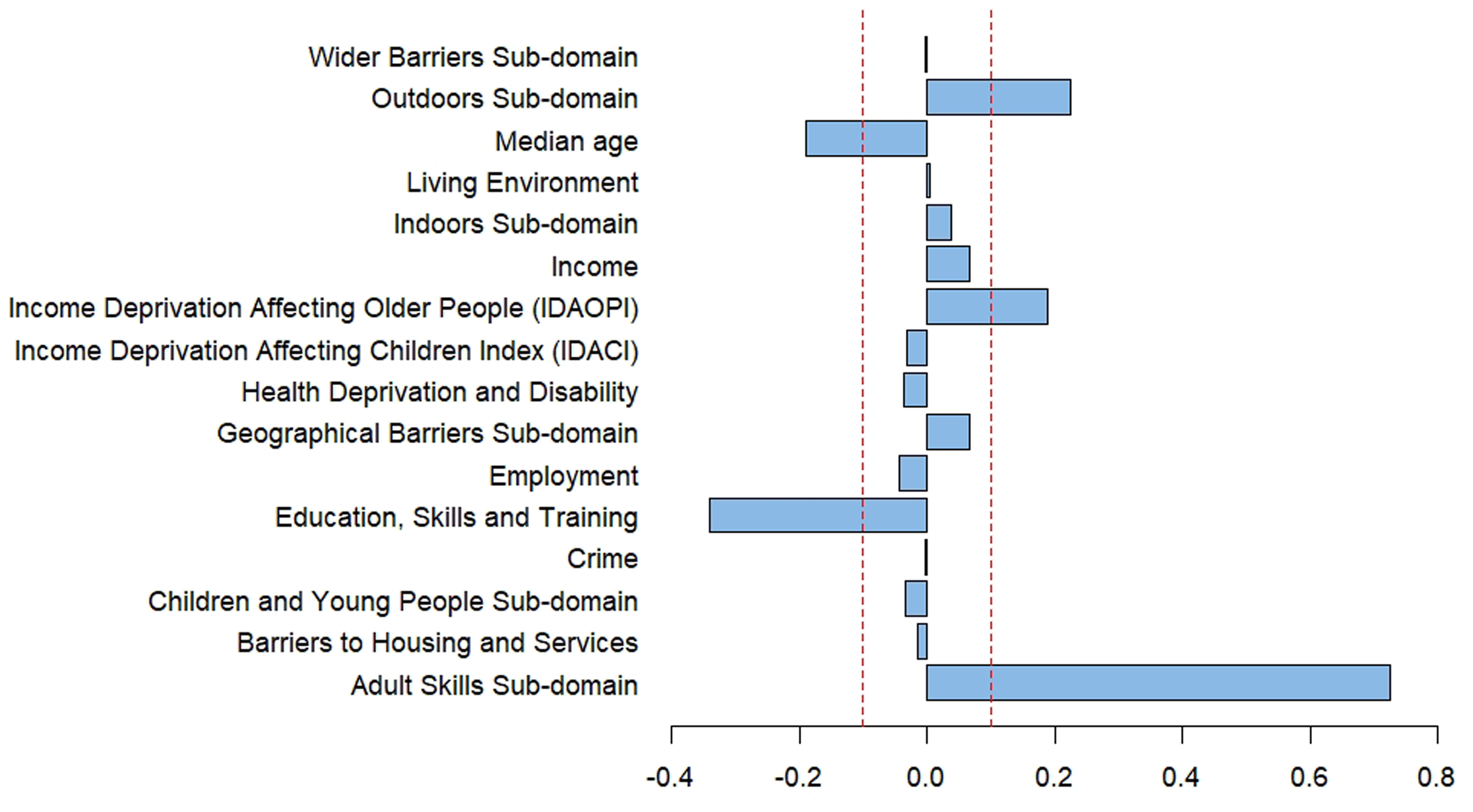

Discussion

In this study we successfully propose a methodology that accurately predicts diabetes prescription volumes for small geographies across the city of Bradford. We demonstrate how publicly available open data from multiple sources can be intelligently linked to enable inferential analysis of prescribing data. Without linked data, the level and depth of analysis achieved in this study would not be possible. Starting with over 217 million records of data, before filtering and processing for the city of Bradford, multiple linear regression and LASSO regression models were trained against published deprivation factors, resulting in high predictive accuracies measured at the LSOA level.

The methodology utilises “Patients registered at a GP practice” data (see Table 1) to infer the geo-spatial distribution of prescribing data at the GP level, then combines data from all GPs in the region to build a narrative of the geography. Our analysis focuses on geographies at the LSOA level, which is typically the most granular level of data available when using publicly available open data.

Multiple linear regression models resulted in an average correlation (from 500 iterations) of R² = 0.672 while LASSO regression improved on this resulting in an average correlation of R² = 0.775. LASSO regression also produced a smaller mean absolute error value, suggesting a more accurate model is achieved using this method. When all 500 iterations of the regression models are considered, multiple linear regression resulted in two independent variables, Outdoors Sub-domain and Median age, that were statistically significant (p-values of ≤0.05). The LASSO regression models predominantly favoured 5 independent variables, Outdoors Sub-domain, Median age, Income Deprivation Affecting Older People (IDAOPI), Education, Skills and Training, and Adult Skills Sub-domain, two of which were statistically significant in the multiple linear regression models too.

Risk factors for diseases such as diabetes include, age, gender, and ethnicity.³⁶ Although gender and ethnicity were not considered in this study, Median age was used and proved significant in both the models tested. The Outdoors Sub-domain variable includes an estimate of air quality based on the concentrations of four pollutants (nitrogen dioxide, benzene, sulphur dioxide and particulates).³⁷ Studies in the literature have reported strong associations with particulate matter pollutants and incidence of diabetes.^11,38,39 These findings seem to corroborate with the outcome of the regression models of this study. The remaining three independent variables (Income Deprivation Affecting Older People (IDAOPI), Education, Skills and Training, and Adult Skills Sub-domain) that the LASSO models chose to use, were all discarded when assessing the multicollinearity between independent variables using the variance inflation factor prior to multiple linear regression analysis. Providing explanatory reasons behind these three variables is yet to be established.

A trade off between model performance and model explainability would be one important consideration when choosing which regression model to use. While LASSO models performed better in model accuracy, it chose independent variables that showed high multicollinearity which would make explainability difficult. LASSO selects the penalty based on it’s cross validation metrics, but if a feature has some additional explanatory power behind it, it will likely remain even if it is closely correlated to another feature. While multicollinearity checks are commonplace in regression analysis, it has been argued that checks may not be necessary if the primary intention of the regression analysis is to build strong predictive models but not to use the coefficients to explain how the dependent variable is affected by each independent variable.⁴⁰ If our multiple linear regression models are trained using all 16 independent features to regress against, i.e., without prior multicollinearity checks and removal of features, the models on average (of 500 iterations) resulted in R² values of 0.8, with lower mean absolute error (0.352) and root mean squared error (0.445) than those of the models reported in this study (see Table 5).

The motivation behind this study was to provide cost saving solutions around diabetes care as identified by the NHS commissioned report for Bradford CCG.¹⁸ The methodology and models proposed have shown high predictive accuracies for the city of Bradford. To validate the methods, we identified other regions of England which may equally benefit from predictive diabetes prescribing models. Using the NHS Quality and Outcomes Framework,⁴¹ three further local authority districts were identified; the city of Birmingham, Ealing which is a district of West London, and the city of Leicester. All three regions are known to have higher than the national average diabetes prevalence.^41,42

Regression models developed from the data of these three regions again resulted in high accuracies, showing the proposed methodology is applicable to a range of geographies and cities. The R² values for the multiple linear regression models were, 0.735, 0.648, and 0.777 for Birmingham, Ealing, and Leicester respectively. The LASSO regression models resulted in R² values of 0.741, 0.613, and 0.792 for Birmingham, Ealing, and Leicester respectively. Similarly, to the city of Bradford models, the Outdoors Sub-domain and Median age were significant variables in both the multiple linear regression and LASSO models. Other variables such as Geographical Barriers Sub-domain and Adult Skills Sub-domain were frequently used by both models (from 500 iterations), however, providing explanatory reasons behind these variables is yet to be ascertained.

Several limitations of this study were identified and should be considered when developing such models, they are discussed herein. The analysis presented in this study works on the hypothesis that drugs prescribed by a GP are distributed in accordance with the GP’s demographic distribution. For the models of this study the approximation works well, producing highly accurate models. For other disease this may not be the case, although further analysis would be necessary to confirm this.

The methodology presented in this study uses the total population of an LSOA region (see equation (4)), and the median age as an independent variable. There are no considerations made for gender or ethnicity, which are known risk factors for diseases such as diabetes.³⁶ If such demographic information are available, the equations and their weightings could be further refined potentially improving the models. Or those variables could be included as part of the independent variables pool. Other factors such as estimating the prevalence of gestational diabetes within a demographic would be beneficial to such analysis also.

When amounting the LSOA total (see equation (3)), only LSOAs served by GPs that reside within the city of Bradford are considered. In actuality there may be a GP residing outside the city of Bradford, with registered patients residing within LSOA regions inside the city of Bradford. In this study, data for those GPs were omitted, which introduces an element of error into the data processing. Ideally GP’s within the entire country should be processed, before filtering data for the LSOA regions of interest. This would ensure no data is missed. Due to processing constraints this study was limited to the city level.

Conclusion

One of the aims of this study was to gauge the usefulness of open data and how linked data could be utilised to again in depth insights. We have successfully demonstrated one such application, but the methodology could be expanded to other diseases or purposes beyond health applications.

Within the city of Bradford alone, we identified through the literature that endocrine nutritional and metabolic problems, which include diabetes, presented a significant area of cost savings, estimated to be in the region of £1.85 million.¹⁸ Predictive models like those demonstrated in this study could play a significant role in authorities being able to forecast and plan resources, be it financial or otherwise, to achieve significant savings for the health services. By identifying geographical areas that show emerging signs of deprivation, early intervention methods could be deployed to prevent an increase in diabetes incidence or forecasts made to estimate the level of public services required to manage diabetes in a given geography or population.

In future work, we aim to further refine these models, in particular around using more detailed demographic data to weigh our data accordingly. Extending these models to other diseases and conditions would be a useful test of the application domain, appropriate to these models.

Footnotes

Declaration of conflicting interests

The author(s) declared no potential conflicts of interest with respect to the research, authorship, and/or publication of this article.

Funding

The author(s) received no financial support for the research, authorship, and/or publication of this article.

Ethical approval

An ethics review of the study was undertaken by the Chair of the School Research Ethics and Integrity Committee in the School of Computing and Engineering at the University of Huddersfield, UK. It was declared that no ethical approval was necessary for this work.

Data availability

This study uses open data made available through official online sources and referenced in the article. Data are publicly available and free to use under an open government license.

ORCID iD

Pritesh Mistry

References

NHS

Digital.

Prescribing for diabetes in England 2008/09 - 2018/19. Source: Office for National Statistics licensed under the Open Government Licence v.3.0), https://digital.nhs.uk/data-and-information/publications/statistical/prescribing-for-diabetes/2008-09—2018-19 (accessed 03 January 2022)

Candler

Mahmoud

Lynn

, et al. Continuing rise of type 2 diabetes incidence in children and young people in the UK. Diabet Med 2018; 35(6): 737–744.

Zghebi

Steinke

Carr

, et al. Examining trends in type 2 diabetes incidence, prevalence and mortality in the UK between 2004 and 2014. Diabetes Obes Metab 2017; 19(11): 1537–1545.

Ogurtsova

da Rocha Fernandes

Huang

, et al. IDF diabetes atlas: global estimates for the prevalence of diabetes for 2015 and 2040. Diabetes Res Clin Pract 2017; 128: 40–50.

Jacobs

Tönnies

Rathmann

, et al. Association between regional deprivation and type 2 diabetes incidence in Germany. BMJ Open Diabetes Res Care 2019; 7(1): e000857. DOI: 10.1136/bmjdrc-2019-000857.

Nishino

Gilmour

Shibuya

. Inequality in diabetes-related hospital admissions in England by socioeconomic deprivation and ethnicity: facility-based cross-sectional analysis. PloS One 2015; 10(2): e0116689.

Covvey

Johnson

Elliott

, et al. An association between socioeconomic deprivation and primary care antibiotic prescribing in Scotland. J Antimicrob Chemother 2014; 69(3): 835–841.

Thomson

Berry

Robinson

, et al. An examination of trends in antibiotic prescribing in primary care and the association with area-level deprivation in England. BMC Public Health 2020; 20(1): 1–9.

Wise

. Antibiotic prescribing is higher in deprived areas of England. BMJ 2015; 351: h6117.

10.

Choi

Lee

, et al. Effect of socioeconomic deprivation on outcomes of diabetes complications in patients with type 2 diabetes mellitus: a nationwide population-based cohort study of South Korea. BMJ Open Diabetes Res Care 2020; 8(1): e000729. DOI: 10.1136/bmjdrc-2019-000729.

11.

Connolly

Unwin

Sherriff

, et al. Diabetes prevalence and socioeconomic status: a population based study showing increased prevalence of type 2 diabetes mellitus in deprived areas. J Epidemiol Community Health 2000; 54(3): 173–177.

12.

Barnard-Kelly

Cherñavvsky

. Social inequality and diabetes: a commentary. Diabetes Ther 2020; 11(4): 803–811.

13.

Office for National Statistics . Census geography. Source: Office for National Statistics licensed under the Open Government Licence v.3.0), https://www.ons.gov.uk/methodology/geography/ukgeographies/censusgeography (accessed 03 January 2022)

14.

El Emam

. Guide to the de-identification of personal health information. Boca Raton, FL: CRC Press, 2013.

15.

El Emam

Rodgers

Malin

. Anonymising and sharing individual patient data. BMJ 2015; 350: h1139. DOI: 10.1136/bmj.h1139.

16.

Diabetes uk , https://www.diabetes.org.uk/about_us/news/diabetes-prevalence-statis (accessed 03 January 2022)

17.

Feltbower

Bodansky

McKinney

, et al. Trends in the incidence of childhood diabetes in South Asians and other children in Bradford, uk. Diabet Med 2002; 19(2): 162–166.

18.

NHS England, https://www.england.nhs.uk/rightcare/products/casebooks/ (accessed 05 January 2022)

19.

Schneeberger

Stöger

Holzinger

. The European legal framework for medical AI. In: International Cross-Domain Conference for Machine Learning and Knowledge Extraction, Dublin, Ireland, 25–28 August 2020. Springer, pp. 209–226.

20.

Curtis

Dennis

Shields

, et al. Time trends and geographical variation in prescribing of drugs for diabetes in England from 1998 to 2017. Diabetes Obes Metabol 2018; 20(9): 2159–2168.

21.

Wilson-Davis

Stevenson

McGavock

. Predicting prescribing costs in general practice using practice demography. Pharmacoepidemiol Drug Saf 1997; 6(3): 189–196.

22.

Wilson-Davis

Stevenson

. Predicting prescribing costs: a model of northern ireland general practices. Pharmacoepidemiol Drug Saf 1992; 1(6): 341–345.

23.

Rabeea

Merchant

Khan

, et al. Surging trends in prescriptions and costs of antidepressants in england amid covid-19. DARU 2021; 29(1): 217–221. DOI: 10.1007/s40199-021-00390-z.

24.

NHS Business Service

Authority.

English prescribing data (EPD). Source: Office for National Statistics licensed under the Open Government Licence v.3.0), https://www.nhsbsa.nhs.uk/prescription-data/prescribing-data/english-prescribing-data-epd (accessed 27 October 2021)

25.

ONSPortal Open Geography . National statistics postcode lookup. Source: Office for National Statistics licensed under the Open Government Licence v.3.0), https://geoportal.statistics.gov.uk/search?collection=Dataset&sort=name&tags=all(PRD_NSPL) (accessed 27 October 2021)

26.

ONS Open Geography Portal. LSOA to wards lookup. Source: Office for National Statistics licensed under the Open Government Licence v.3.0), https://geoportal.statistics.gov.uk/search?collection=Dataset&sort=name&tags=all(LUP_LSOA_WD) (accessed 27 October 2021)

27.

NHS

Digital.

Patients registered at a GP practice october 2019; special topic - practices that have closed since October 2018. Source: Office for National Statistics licensed under the Open Government Licence v.3.0), https://digital.nhs.uk/data-and-information/publications/statistical/patients-registered-at-a-gp-practice/october-2019 (accessed 27 October 2021)

28.

Office for National Statistics . Lower layer super output area population estimates. Source: Office for National Statistics licensed under the Open Government Licence v.3.0), https://www.ons.gov.uk/peoplepopulationandcommunity/populationandmigration/populationestimates/datasets/lowersuperoutputareamidyearpopulationestimates (accessed 27 October 2021)

29.

GOVUK.

English indices of deprivation 2019. Source: Office for National Statistics licensed under the Open Government Licence v.3.0), https://www.gov.uk/government/statistics/english-indices-of-deprivation-2019 (accessed 27 October 2021)

30.

NICE . BNF publications, https://www.bnf.org/ (accessed 27 October 2021)

31.

R Core Team . R: A language and environment for statistical computing, https://www.R-project.org/ (2017, accessed 25 March 2021).

32.

Freedman

. Statistical models: theory and practice. Cambridge, UK: Cambridge University Press, 2009.

33.

Tibshirani

. Regression shrinkage and selection via the lasso. J R Stat Soc: Series B (Methodol) 1996; 58(1): 267–288.

34.

Bruce

. Practical statistics for data scientists. Sebastopol, CA: OREILLY, 2017.

35.

Nordhausen

. An introduction to statistical learning—with applications in R by Gareth James, Daniela Witten, Trevor Hastie & Robert Tibshirani. Wiley Online Library, 2014.

36.

Pham

Carpenter

Morris

, et al. Ethnic differences in the prevalence of type 2 diabetes diagnoses in the uk: cross-sectional analysis of the health improvement network primary care database. Clin Epidemiol 2019; 11: 1081.

37.

GOVUK.

English indices of deprivation 2019: research report. Source: Office for National Statistics licensed under the Open Government Licence v.3.0), https://www.gov.uk/government/publications/english-indices-of-deprivation-2019-research-report (accessed 27 October 2021)

38.

Bowe

Xie

, et al. The 2016 global and national burden of diabetes mellitus attributable to PM_{2 5} air pollution. Lancet Planet Health 2018; 2(7): e301–e312.

39.

Meo

Memon

Sheikh

, et al. Effect of environmental air pollution on type 2 diabetes mellitus. Eur Rev Med Pharmacol Sci 2015; 19(1): 123–128.

40.

Siegel

. Practical business statistics. Cambridge, MA: Academic Press, 2016.

41.

NHS digital, https://digital.nhs.uk/data-and-information/publications/statistical/quality-and-outcomes-framework-achievement-prevalence-and-exceptions-data (accessed 03 January 2022)

42.

UK Parliament, https://commonslibrary.parliament.uk/diabetes-in-england-where-are-the-hotspots/ (accessed 03 January 2022)

Prediction of diabetes prescription volumes of various geographies using regression techniques

Abstract

Keywords

Introduction

Method

Data

EPD data

National statistics postcode lookup data

LSOA to wards data

Patients registered at a GP practice data

LSOA population estimates data

Indices of multiple deprivation data

Data processing

Regression model analysis

Multiple linear regression

LASSO regression

Results

Multiple linear regression model

LASSO regression models

Discussion

Conclusion

Footnotes

Declaration of conflicting interests

Funding

Ethical approval

Data availability

ORCID iD

References