
Abstract
Accurate demand forecasting is always critical to supply chain management. However, many uncertain factors in the market make this issue a huge challenge. Especially during the current COVID-19 outbreak, the shortage of certain types of medical consumables has become a global problem. The intermittent demand forecast of medical consumables with a short life cycle brings some new challenges, such as the demand occurring randomly in many time periods with zero demand. In this research, a seasonal adjustment method is introduced to deal with seasonal influences, and a dynamic neural network model with optimized model selection procedure and an appropriate model selection criterion are introduced as the main forecasting models. In addition, in order to reduce the impact of zero demand, it adds some input nodes to the neural network by preprocessing the original input data. Lastly, a modified error measurement method is proposed for performance evaluation. Experimental results show that the proposed forecasting framework is superior to other intermittent demand models.
Keywords
Introduction
Demand could be smooth, intermittent, lumpy, erratic and slow-moving. 1 In the past few decades, many researchers have proposed different indicators to categorize demand types. The two most popular indicators are Average inter-Demand Interval (ADI) and Coefficient of Variation (CV). 1 A lot of methods have been proposed to cope with the forecasting of different demand patterns.2–4 Generally, if the average number of time periods between two non-zero demands is 1.25 times the number of the inventory review period, the demand can be considered as intermittent demand. 5 Traditional forecasting techniques, such as simple exponential smoothing or simple moving average, are inappropriate for intermittent demand. 6 This paper will focus on new methods that can forecast the intermittent demand for medical consumables with short life cycle, which may help supply chain decisions during the COVID-19 epidemic.
Intermittent demand is usually related to engineering spares, service parts and high-priced capital goods, such as heavy machinery. 7 In recent years, research on customized short-life medical consumables has attracted attentions from global scientists from all over the world. The main characteristics of this typical medical consumables are short lifecycle, large proportion of zero daily demands, various product styles and long replenishment lead time, which are very similar to the fast fashion industry 1 in certain aspects, and it also brings a lot of challenges to the supply chain management around world. Demand forecasting is of great importance in controlling the inventory of such products, but the intermittent and slow-moving nature of demand makes forecasting particularly difficult.
Motivated by a real business analytics project, we propose a new method to forecast the intermittent demand. Our study arises from a manufacturer of medical consumables that operates a warehouse and a couple of retail stores in Asia. Since the demand for medical consumables is usually erratic, we introduce the techniques of dropping outliers, seasonal adjustment and aggregation to preprocess historical data. In addition, a new forecast accuracy measurement is proposed specifically for the zero demand records and a dynamic neural network is designed to handle the erratic and unstable demand data.
The remainder of this study is structured as follows. In Section 2, the overview of relevant research and existing literature is provided. Section 3 introduces the main forecasting models, accuracy measurements and competing intermittent demand forecasting methods. In Section 4, the experimental and computational results are reported, including descriptive analysis of real data set, data preprocessing, experiment implementation and results analysis. Section 5 concludes this study with some remarks and future research directions.
Literature review
In this section, we mainly review previous work on data aggregation, demand forecasting, model optimization and selection.
Data aggregation
The main challenge of intermittent demand forecasting lies in the large proportion of zero demands. An intuitive way dealing with such pattern is to aggregate demands. The data from the company of this study reveals that most product demand is intermittent. Therefore, it is very difficult to use the original sales data in the point-to-sale (POS) system of each individual store to make forecasting directly. Data aggregation is usually conducted before applying forecasting methods.8,9 An important decision that should be made is to aggregate the dimensions and levels of sales data. There are three possible dimensions for aggregation, namely the time dimension, the product hierarchical classification (i.e. product tree)8–10 dimension and the sales channel dimension. In the time dimension, the aggregation level can be day,11,12 week, 13 month9,14–16 or year.17,18 In the product hierarchical classification dimension, the aggregation level can be SKU, 15 article (a group of SKUs under the same product number but with different sizes and colors), 19 product family/group (e.g. shoes, apparel, or accessories),11,13,14,18 attribute values (such as the color being red or black, or the size being large, small, or middle),13,17,19 or the assortment of the overall supply chain. 16 In the sales channel dimension, the aggregation level can be store, 12 , all stores in the supply chain,13–18 or a set of stores in a region/city that is a part of the supply chain. 11 The aggregated data sets for different levels in each dimension often have different features in smoothness, intermittence, lumpiness and slow-moving. For example, the daily sales data sets for all SKUs and all stores are very likely to be smooth. Different aggregation levels in each dimension may require different forecasting methods and have different influences on forecasting accuracy. 8 In Table 1, we summarize the aggregation levels in existing literature on short life cycle product sales forecasts.
Summary of the aggregation levels in the three dimensions.
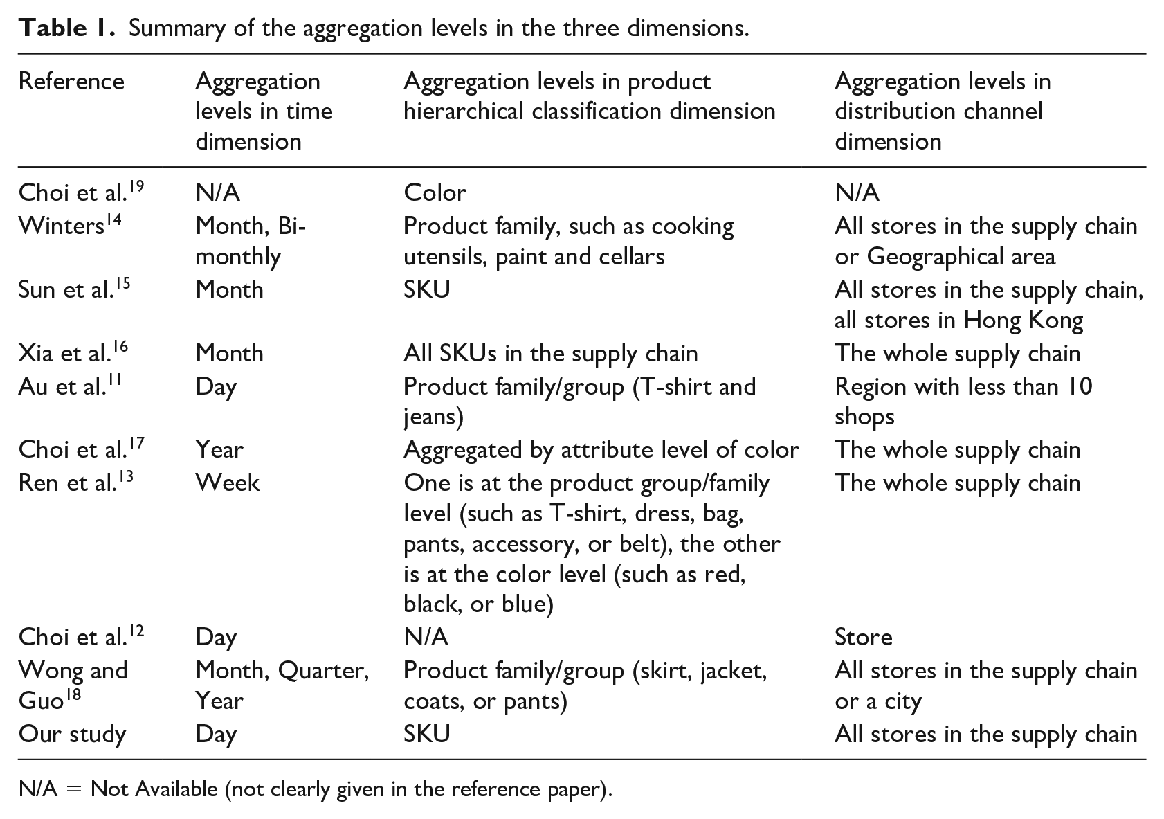
N/A = Not Available (not clearly given in the reference paper).
Nikolopoulos et al. 20 proposed a framework, called ADIDA, to optimize the aggregation level. ADIDA is an empirical framework, not a theoretical framework, which only considers the aggregation of time dimension. The time dimension has to consider the lead time. 21 In the dimension of product hierarchical classification, the products themselves and the manufacturing procedure should be considered, so that the aggregation improves the manufacturing efficiency. For instance, if the aggregation level in the product hierarchical classification dimension is a color level, and the painting procedure precedes the manufacturing procedure, the aggregation does not make sense because managers must determine the quantity of each color during the manufacturing process. Lastly, in the distribution channel dimension, three levels can be considered, namely store, region and supply chain. The selection of distribution channel dimension also needs to consider the manufacturing procedure. In short, data aggregation is a systematic work, and various aspects should be considered. Syntetos et al. 22 established a supply chain structure, which includes four dimensions for supply chain forecasting, namely product dimension, location dimension, time dimension and echelon dimension. Figure 1 depicts the three dimensions of data aggregation, where each small block represents one choice of data aggregation. In this study, we select SKU-Day-Chain level to aggregate the demand according to the discussion with managers.
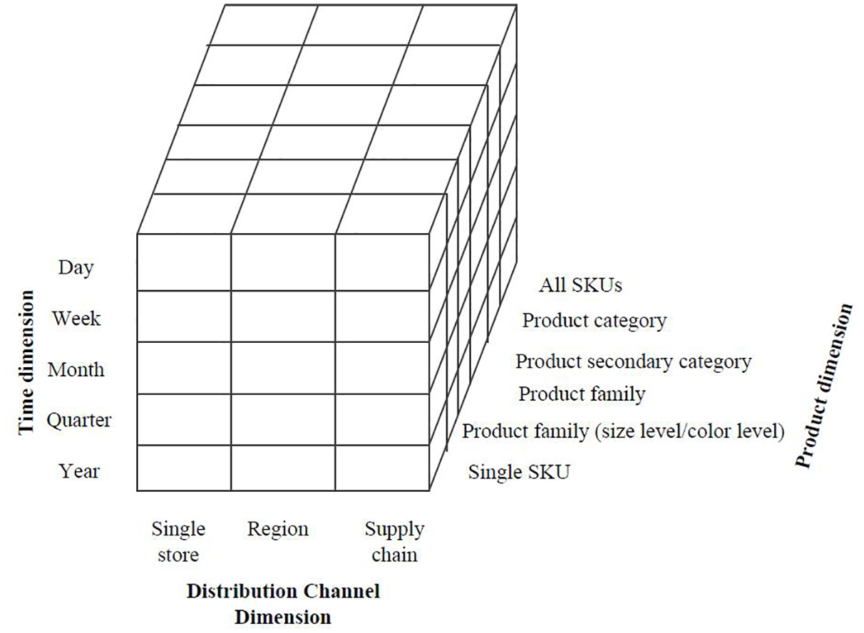
Data aggregation structure.
Demand forecasting
Most of the previous studies dealing with intermittent demands has focused on inventory management and employed appropriate forecasting methods to predict future demands. It should be noted that these forecasting methods are based on the assumption that future demand follows a standard probability distribution, such as Poisson or Negative Binomial distribution. However, real data in the industry often indicates that demand does not satisfy those standard distributions. Thus, these assumption-based forecasting methods performed poorly on real industrial data sets.7,20 Various models have been applied to intermittent demand forecasting. For example, single exponential smoothing and simple moving average are often employed in practice to handle intermittent demands. However, Croston 23 demonstrated that traditional forecasting methods, such as Single Exponential Smoothing, did not perform well for intermittent demand, so a more suitable method, the Croston method, was proposed. Their experiments have shown that Croston’s method outperforms traditional forecasting methods for intermittent demand. Later,5,24 modified the original Croston’s method to improve the forecasting accuracy.
In recent years, specially designed consumables have become more and more popular. One of the most typical characteristics of such products is the short life cycle, which makes historical sales data very limited. Due to the short life cycle, inventory management is very crucial, and the demand forecast of medical consumables with short life cycles is also very difficult. To address this challenge, extensive research has been conducted on the sales forecasts of such products in the existing literature.1,25 Numerous sales forecasting methods have been proposed, such as moving averages and exponential smoothing, 26 Holt-Winters exponential smoothing, 14 autoregression, artificial neural networks, extreme learning machines,15,16 evolutionary neural networks, 11 the hierarchical Bayesian approach, 27 and hybrid model. 12 More detailed and extensive reviews on these forecasting methods can be found in Nenni et al., 1 Thomassey, 9 and Liu et al. 25 Liu et al. divided sales forecasting methods into three groups, namely statistical forecasting methods, advanced statistical learning forecasting methods and hybrid forecasting methods. The advantages and disadvantages of each type of forecasting method are discussed in Liu et al. 25 The statistical forecasting methods are simple and fast, but they cannot produce good results because they cannot handle irregular patterns. Although advanced statistical learning forecasting methods have a stronger ability to identify irregular patterns than statistical forecasting methods, they are time-consuming and require sufficient data. Therefore, they are inappropriate for such products because usually there are a large number of different products for short life cycle medical consumables, and future demand needs to be predicted promptly. In terms of calculation speed, hybrid forecasting methods perform the worst because they include not only advanced statistical learning forecasting procedure, but also other processes.
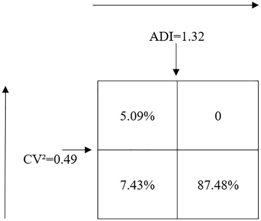
It should be noted that due to several factors such as short life cycle, short selling seasons and long replenishment lead times, the sales data sets of specially designed consumables are usually highly unstable and limited in size.1,8,9,19 The concepts of intermittent data and such product sales data are not equivalent because the data may not be intermittent. Many previous works have been established to classify demand patterns.28–30 As shown in Figure 2, we employ the method in Syntetos et al., 29 which uses two indicators, namely ADI and CV, to recognize intermittent demands.
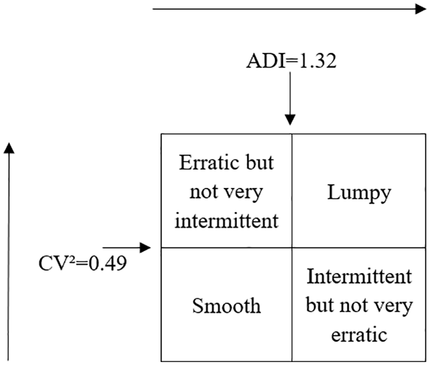
Classification of demand patterns.
Model selection
Some researchers have investigated how to optimize the forecasting model of intermittent demand.31,32 Another research direction similar to model specification in statistics is model selection. The purpose of model specification and selection is to find the most suitable model for a given data set. Some methods for selecting intermittent demand models based on data characteristics have been proposed by Kostenko and Hyndman 28 and Heinecke et al. 30 Furthermore, Kourentzes 33 investigated whether different accuracy measures can facilitate and automate the model selection for intermittent demand data.
There are few researches on optimizing the forecasting model for short life cycle products. 11 proposed a modified evolutionary neural network to conduct forecasting for a fashion retailer, which is faster than the original evolutionary neural network. However, the model in Au et al. 11 is still time-consuming and may not converge to the optimal result.
In brief, model selection is very important to forecast the demand for such short life cycle products because of the considerable irregularity in their sales data. In our research, we propose a new forecasting accuracy measure for the model to deal with zero demand, and introduce a dynamic neural network, minimum description length neural network (MDL-NN), as the core part of the forecasting model. MDL was originally used for data compression,34,35 which is a technique from algorithmic information theory, which indicates that the best hypothesis for a given data set is the assumption that results in maximum data compression. One seeks to minimize the sum of length, which includes an effective description of the model and length, and an effective description of the data when coding with the model. 35 In time series forecasting, the description length of a model is the sum of the model description length and the model prediction error. MDL-NN searches for the optimal model size (i.e. the number of neurons in neural network), and avoids overfitting or underfitting by minimizing the model’s description length and its performance. 34
Methodologies
Our proposed demand forecasting model
In this section, our proposed demand forecasting model will be introduced. This demand forecasting model mainly includes three parts, the first part is the basic forecasting model, the second part is the criterion about the optimal model, including when the model selection procedure should be stopped, and the last part is the optimized model selection procedure. Since the model selection problem is an NP-hard problem, we cannot search all candidate models. Thus, the optimized model selection procedure can effectively accelerate the search for optimal model. Lastly, we propose a framework for the demand forecasting model employed in our research.
Basic forecasting model
Neural network as a flexible model was employed in our study. The activation functions are radial basis functions, since we design a flexible neural network, initially, both linear radial basis functions and nonlinear radial basis functions are included in neural network model. Without loss of generality, let
Then the new input data is
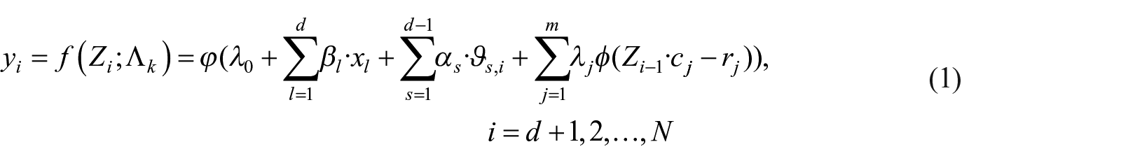
where

Criterion of optimal model
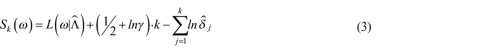
In order to select optimal neurons in neural network, the minimum description length (MDL) is adopted as a criterion to select the optimal neural network. The number of neurons in the hidden layer determines the complexity of the neural network, and selecting the most appropriate number of neurons becomes a challenge and important task when optimizing the architecture of neural network. According to bias-variance trade-off theory, if the model is too simple and includes very few parameters relative to data, then it will have large bias, we call that underfitting, and then model cannot completely capture the data patterns. 36 While if the model includes very many parameters relative to data, then it will suffer from large variance, we call that overfitting, the model performs well on the training data, but bad on the test data. Therefore, we employ a criterion to select optimal model to avoid overfitting or underfitting problem. The original expression of MDL 37 is presented as follow:
where

The above criterion is the same with Schwarz’s criterion 39 in form but not in scope nor in content. 38
Optimized model selection procedure
In this section, optimized model selection procedure will be introduced, which adopted sMDL to selection optimal neural network. As we have mentioned before, the search of optimal model is a NP-hard problem, effective search algorithm should be employed to handle this problem. The main algorithm is searching for the optimal number of neurons by iteratively adding and removing neurons until the model reach the criterion of sMDL. Thus, we have no need to set the number of neurons in the hidden layer in advance. The detailed procedure of selecting the optimal nodes in neural network model is presented as follow:
Step 1: Let
Step 2: Compute the weights
Step 3: To find optimal neurons in the hidden layer, we generate a set of candidate nonlinear neurons
Step 4: To select the best candidate neurons, we find the basis function
Step 5: Let
Step 6: Add a new neuron in the hidden layer. If there is a neuron that fits the current error worse than the new neuron, then that neuron should be abandoned, namely, find
Step 7: If
Step 8: The weights
Step 9: If the minimal sMDL in equation (4) is reached, then stop, or else, go to step 3.
The framework of demand forecasting
The framework of our demand forecasting method is presented in Figure 3. The detailed steps are described as follows:
Step 1: Aggregate data based on the original data set;
Step 2: Preprocess data;
Step 3: Select the optimal neural network for the sales time series of each product;
Step 4: Conduct forecasting for each time series;
Step 5: Calculate forecasting accuracy and significance test of performance for different models.
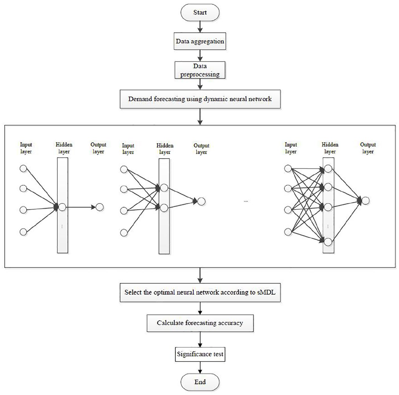
The framework of our demand forecasting method.
Forecasting accuracy measurements
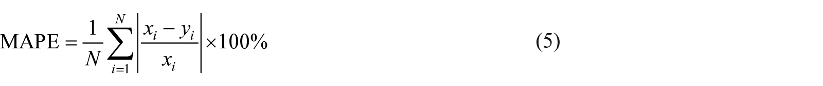
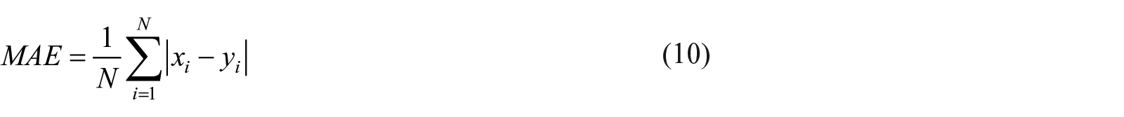
To evaluate the forecasting methods, we use some common measurements, including mean absolute percentage (MAPE), symmetric mean absolute percentage error (SMAPE) and mean absolute error (MAE). Although several studies proposed new measures to particularly evaluate the forecasting methods for intermittent demand,40,41 very few of them paid attention to the large proportion of zero values. Prestwich et al. 42 proposed some mean-based measurements for intermittent demand. The most widely used measure is MAPE whose mathematical expression is:
where
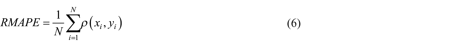
where
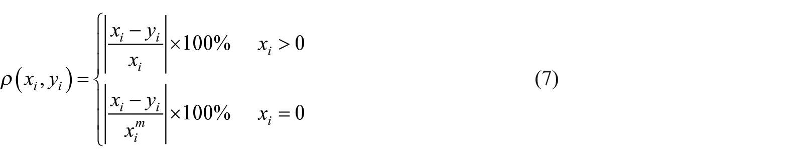
Where
In addition to the proposed RMAPE, we use two other measures, namely SMAPE and MASE, which also address the issue of zero sales records, we replace SMAPE by RSMAPE to eliminate the effect of zero. These two methods are defined as:

where
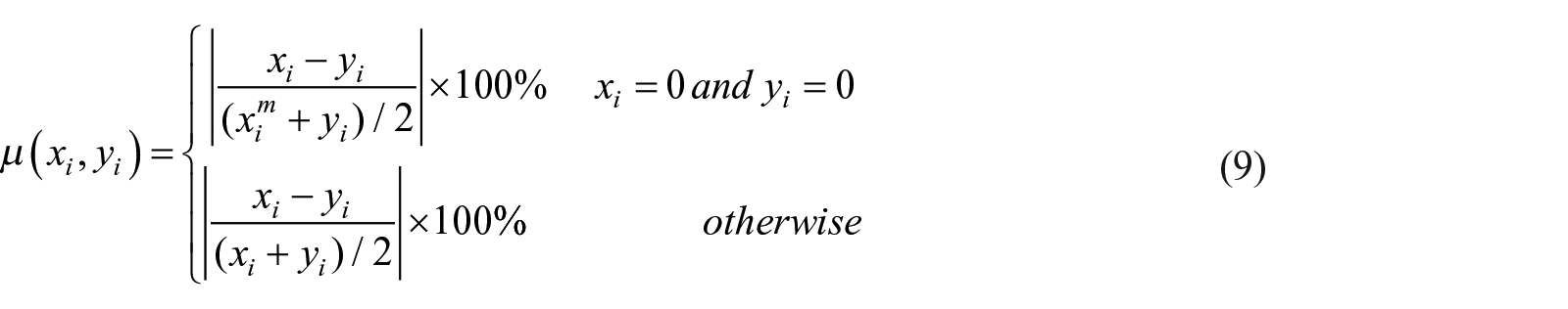
Where
Competing methods
Five other widely used forecasting methods for the demand of short life cycle products, namely gray model (GM), extreme learning machine (ELM), support vector machine (SVM), Markov regime switching (MS), Syntetos and Boylan’s method and neural network in equation (1) without optimized model selection procedure are applied to our data sets for comparative analyses. The GM was first introduced by Deng
44
and used for demand forecasting in.17,45 This method has two parameters
Numerical investigation
In this section, Numerical investigation will be conducted. We first describe a data set of a real medical consumable retailer, and then report detailed information on data preprocessing, experiment implementation, result analysis and significant test.
Data
Our data set comes from a point of sale (POS) system from the retail stores of a manufacturer of medical consumables under a non-disclosure agreement. The time horizon ranges from January 1, 2012 to July 20, 2014. We present some descriptive statistics on the data set in Table 2.
Descriptive statistics of all data.
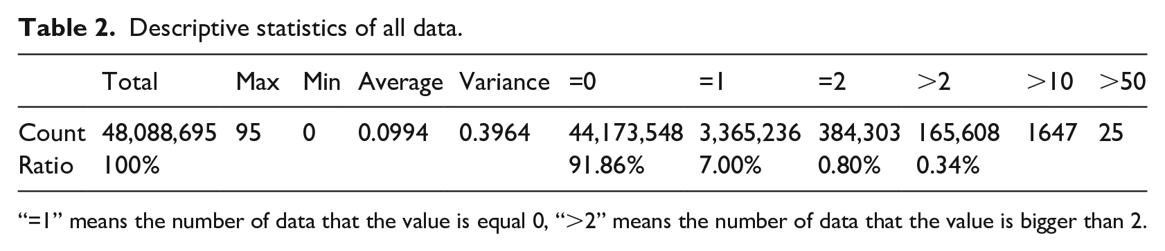
“=1” means the number of data that the value is equal 0, “>2” means the number of data that the value is bigger than 2.
Table 2 shows that 91.86% of the total sales records have a zero demand. According to demand classification in Figure 2, we can show the distribution of demand patterns in our data set in Figure 4. From this figure, we can know that the majority of the demands in the data set are intermittent. Thus, we have to aggregate the daily sales records of each SKU at the supply chain level. After aggregation, each record represents the total sales of a certain SKU in all retail stores. Then the descriptive statistics of the aggregated data is presented in Table 3.
The distribution of demand patterns in the data set.
Descriptive statistics of the aggregated data at the supply chain level.
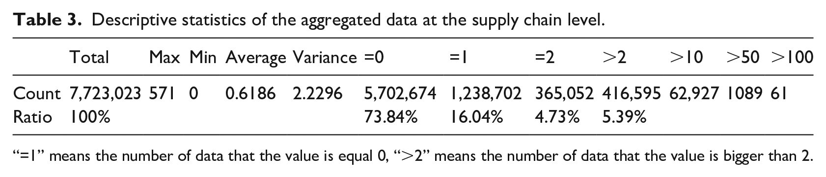
“=1” means the number of data that the value is equal 0, “>2” means the number of data that the value is bigger than 2.
For the aggregated data, we need to pay attention to the following three aspects. First, around three-quarter of the sales records are still zero and thus data is still sparse. Second, that the maximum demand is 571 implies the existence of the outliers. Third, the fact that many records have large demand sizes may be caused by the seasonal factors or sales promotion. Therefore, we drop outliers and conduct seasonal adjustments before forecasting the demand.
Data preprocessing
The data preprocessing includes deleting outliers and records with missing values. For simplicity, Tukey’s Boxplot 49 is adopted to determine whether a certain value is an outlier. Moreover, we represent the outliers by the mean of its before and after value. Then, we employ the multiplicative seasonal decomposition approach, 50 which is the most common way, to conduct seasonal adjustment. 50 Lastly, we normalize the sales time series for each SKU separately using the unity-based normalization method.
Implementations
Before applying seven methods discussed in Section 3, we divide the data sets into training and test data sets. The former 66% of the data is the training data set, and the remaining 34% is the testing data set. Since the forecasted values by these methods are decimal numbers, we round them to their nearest integer. When calculating the three-performance indicators, we consider both the forecasted decimal values and the rounded integral values. Lastly, encompassing test is further employed to indicate the capabilities of different models.
Results and analysis
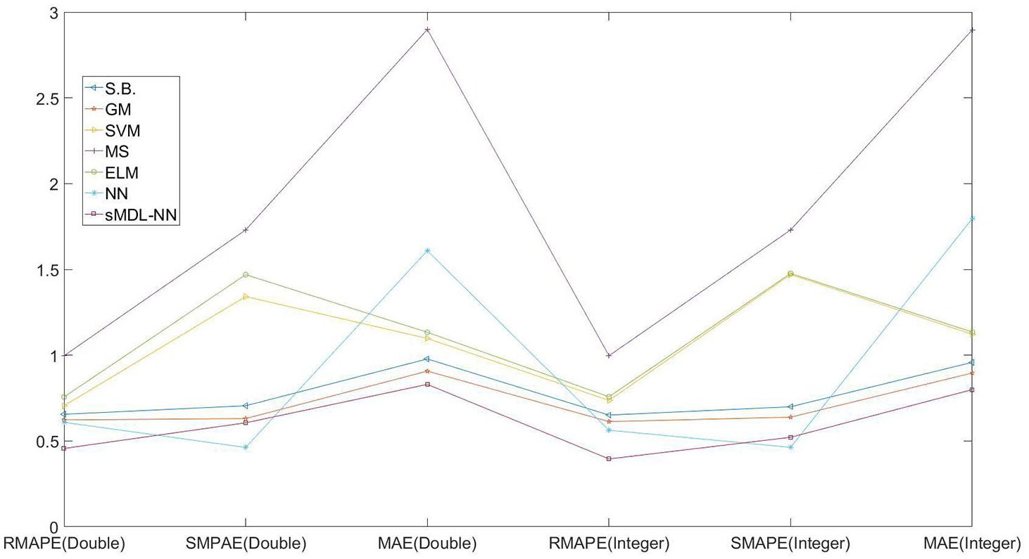
To our knowledge, no other studies have discussed the influence of different formats of results on the accuracy of forecasting methods. The demand forecasted by advanced statistical learning and statistical methods is commonly presented in decimal number. However, only integral demand of SKUs can be ordered or delivered. So, in practice the decimal numbers need to be rounded to their nearest integers. When the demand is large, the difference between decimal and integral numbers has little effect on the result. But this difference matters for short life cycle products as the demand size of such products is usually very small (e.g. most of sales quantities are 0, 1 or 2). By experiments, we demonstrate that different result formats can lead to different accuracies and thus affect the selection of the appropriate forecasting methods. The computational results produced by the seven methods are shown in Table 4. Columns 2-4 display the decimal values of the RMAPE, RSMAPE, and MASE, respectively, associated with the forecasted decimal results. Columns 5-7 report the corresponding accuracies associated with the integral results. Figure 5 presents the results in Table 4 intuitively. According to the measurement of RMAPE and MAE, the best model is sMDL-NN. In our problem, since a lot of demand is zero, and RMAPE and SMAPE cannot give managers the intuitive judgment based on the results. Thus, MAE is the most accurate measurement in this problem, which can directly provide results for managers, and managers can make decisions accordingly.
Performance for different models.
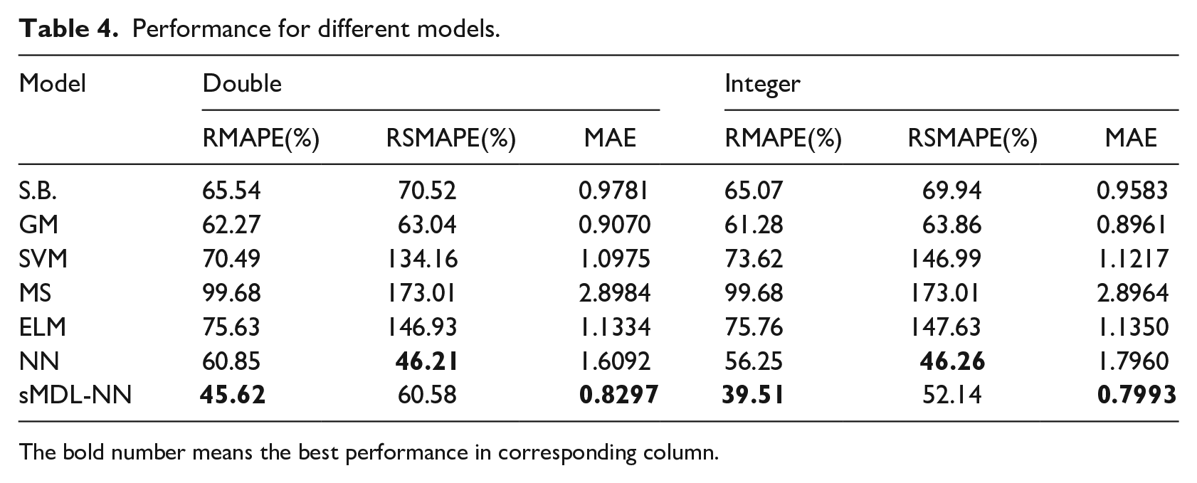
The bold number means the best performance in corresponding column.
Performance for different models.
Encompassing test
In this study, to illustrate the ability of different models in Table 4 further, we introduce the encompassing test51,52 to determine whether forecast encompassing between different models occurs. According to Chong-Hendry forecast encompassing test, if model
Encompassing test for different models.
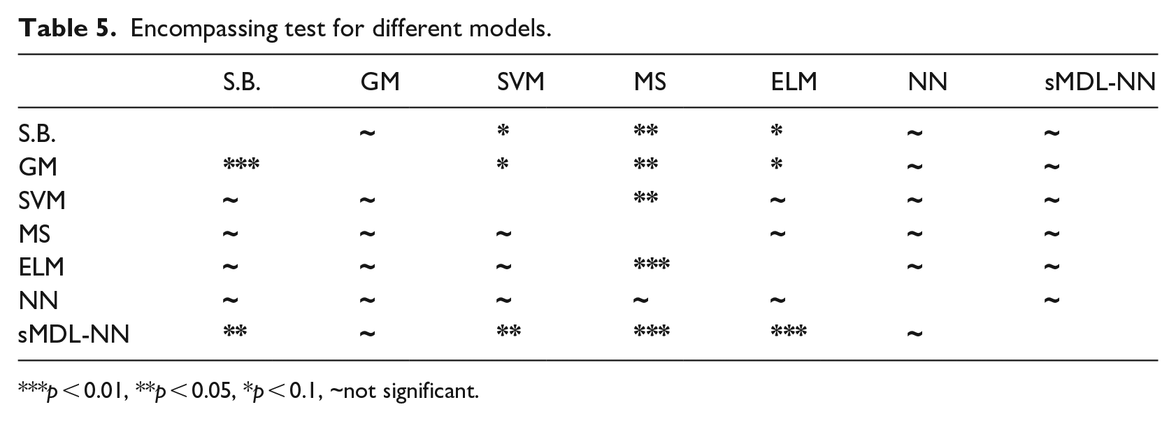
p < 0.01, **p < 0.05, *p < 0.1, ~not significant.
The label in Table 5 indicates whether the model of corresponding row encompasses the model of corresponding column. For instance, GM encompasses S.B., but S.B. does not encompasses GM. In Table 5, our proposed model sMDL-NN has shown the strongest encompassment ability. However, no model can encompass all models in Table 5.
Conclusions
For the intermittent demand forecasting problem of medical consumables with a short life cycle, this study provides a dynamic neural network model based on optimized model selection procedure to select optimal structure of neural network. One critical issue we have to address is to avoid underfitting and overfitting, especially in our limited historical data, which is essentially the problem of model selection. An appropriate model selection criterion is introduced to determine the optimal model. In order to tackle the problem of erratic demand, dropping outliers, seasonal adjustment techniques and aggregation technique are introduced. In addition, a new forecasting accuracy estimator is proposed to improve the generalization capability of zero-demand data.
Six other benchmark methods are also applied, namely Syntetos and Boylan’s method, GM, SVM, MS, ELM and NN. Our experimental results show that the performance of our proposed method outperforms others. Our findings suggest that due to the complexity of sales data, managers should consider model selection, and sMDL-NN is an ideal candidate model to achieve this goal.
The numerical investigation is conducted at the supply chain level. Experimental results and encompassing tests indicate that our proposed sMDL-NN model is superior. The forecasting results of the proposed RMAPE are consistent with MAE.
Another important finding from our study is that different formats of forecasted sales values, such as decimal or integer, can lead to significantly different performance in small demand problems. Although it is common for forecasting methods to use decimal number sales values, in reality only integers can be used because we cannot order or deliver a part of the SKU.
Even this problem is a classical problem, it will not have much influence when the sales data is large. However, in the industry of short life cycle product sales, the demand is usually very small, and then, the forecast sales value of different formats of forecast methods may lead to different decisions. We find that the format of the values should not be ignored, and our experimental results show the gap between the different formats.
Intermittent demand management is a very complicated issue. Further research can be to integrate the forecasted results into inventory, logistics distribution, and pricing operations, such as markdown decisions, to develop models and algorithms to solve practical problems.
Footnotes
Declaration of conflicting interests
The author(s) declared no potential conflicts of interest with respect to the research, authorship, and/or publication of this article.
Funding
The author(s) disclosed receipt of the following financial support for the research, authorship, and/or publication of this article: This research is supported by the National Natural Science Foundation of China (Nos. 71531009).