
Abstract
This work presents an analysis of 3.5 million calls made to a mental health and well-being helpline, seeking to answer the question, what different groups of callers can be characterised by specific usage patterns? Calls were extracted from a telephony informatics system. Each call was logged with a date, time, duration and a unique identifier allowing for repeat caller analysis. We utilized data mining techniques to reveal new insights into help-seeking behaviours. Analysis was carried out using unsupervised machine learning (K-means clustering) to discover the types of callers, and Fourier transform was used to ascertain periodicity in calls. Callers can be clustered into five or six caller groups that offer a meaningful interpretation. Cluster groups are stable and re-emerge regardless of which year is considered. The volume of calls exhibits strong repetitive intra-day and intra-week patterns. Intra-month repetitions are absent. This work provides new data-driven findings to model the type and behaviour of callers seeking mental health support. It offers insights for computer-mediated and telephony-based helpline management.
Keywords
Introduction
Helplines are key elements of mental health and well-being and suicide prevention efforts; however, little is known about how these services are used.
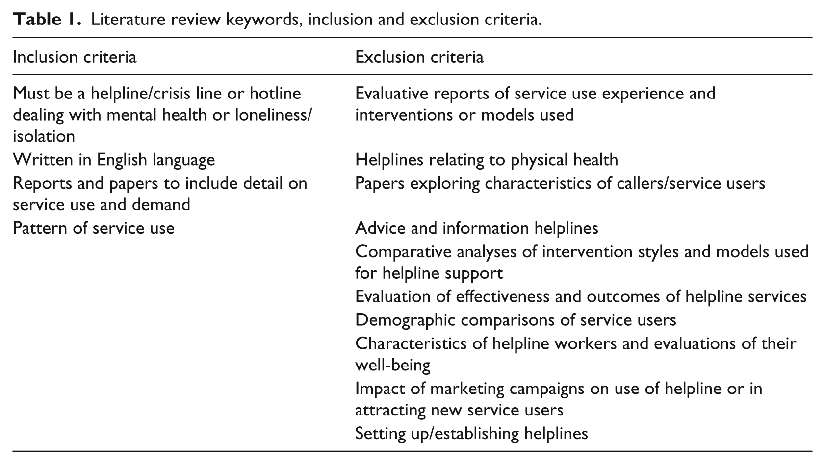
A review of the literature focused on previous research topics, including crisis lines, helplines and hot lines. In all, 16,288 papers were identified through a database and hand search and this was reduced to 21 relevant papers following a two-stage screening process and application of a strict inclusion and exclusion criteria. Table 1 shows the inclusion and exclusion criteria.
Literature review keywords, inclusion and exclusion criteria.
Several themes were identified across the relevant research from the review:
Caller categorization: Most research attempted to categorise callers in some way.
Call duration: Studies categorising calls by duration found that 54 per cent of calls were less than 30 min and 46 per cent of calls were more than 30 min.
Period of service use: Several studies reviewed how long service users were in contact with the service.
Call demand: Most research reported that calls to helplines peaked at weekends and in the evening during the week.
Frequent caller characteristics: Several studies, mainly from Australia identified the behavioural characteristics of repeat and frequent callers.
Reason for calling the service. Studies identified factors that drive frequent callers to call the service including positive reinforcement, isolation, anonymity and unrestricted access.
Influences on call demand: Most helplines reported increased calls across the reported periods. The impact of media was identified in two studies as a key way to encourage people to contact helplines.
The review of the literature indicated that caller behaviour had been the subject of several studies. Research has classified callers as ‘one-off’ or ‘repeat callers’ and studies found that 3 per cent of callers take up 47–60 per cent of the service capacity. 1 In 2010, Samaritans reported 47.7 per cent of calls were ‘snap’ or silent calls. 2 A 2012 study 3 reported that half of its callers contact Samaritans in a given month. Most research on call demand reported that calls to helplines peak at weekends and in the evening during the week. This ranged from 54–68 per cent across helplines.4,5
Two Australian studies identified three different helpline caller types: addicted callers who call out of habit, callers seeking access to emotional support and reactive callers who call when they become unsettled by external triggers. These studies also identified factors that drive frequent callers to call the service: positive reinforcement, social isolation of the caller, service maintaining anonymity of the caller and unrestricted access to the service.6,7
Helplines Partnership identified a trend of increasing demand in UK helplines year on year. 5 Samaritans Ireland reported a 60 per cent increase in demand when they moved to a free phone number in 2014. Analysis of a toll-free crisis line in South Africa highlighted the strong influence of the media as one of the main sources of information about and how service users became aware of the helpline. 8 A report on multiple helplines also reported an increase in the complexity in calls received. 9
Several of the studies reviewed above related to caller behaviour derived from a large telephony dataset. However, these studies focused solely on frequent callers only. No research was found that incorporated analysis of a large dataset over a prolonged multi-year period to provide an understanding of general call patterns and caller behaviour.
The research presented in this article expands upon previous research by analysing a large data sample over a 3-year period and by focusing primarily on service user’s behaviours and how and when they contact the helpline.
Research questions
The review of the literature identified research from helpline providers on user experiences in calling helplines, limited call analysis research that related specifically to frequent callers as well as some general usage statistics for helplines. The review also highlighted that there is no research available that examines all caller behaviours for a mental health helpline, encompassing several years of caller data. This study extends previous research by analysing much larger datasets and examining all caller behaviours. This research aims to provide a greater understanding of call behaviour of all callers seeking mental health and well-being support. The research question, then, that defines the study is, ‘In mental health helplines, what different groups of callers can be characterised by specific usage patterns?’ A related research question is, ‘If identified, then do such groups of usage patterns change over time?’
Context of the current study
This study involves analysis of digital telephony data sourced from Samaritans Ireland, which is a charity with a helpline to provide emotional support to anyone in distress or at risk of suicide. While the charity offers support via texts, email and face to face, ~95 per cent of their contacts remain via telephone. Data were provided for all calls made to the helpline in the Republic of Ireland for almost a 4-year period (April 2013 to December 2016). A total of 3.449 million calls was analysed. This amounts to 725 calls per 1000 population.
The helpline dataset comprises a number of fields; however, only the following fields were used in this study:
Date-time stamp of the call arrival precise to the last second,
Engaged flag meaning that the call was dropped with a busy tone,
Answered flag meaning that the call was passed to a helpline volunteer,
Duration of the call in seconds and
Unique caller ID.
The caller IDs allowed us to enumerate the callers uniquely while providing no personally identifying or sensitive details. In this sense, we could tell ‘who’ was calling. The dataset carried caller ID information for most, but not all, call arrivals. See detail in Table 2.
Caller ID and call volume counts in the helpline dataset: by year and total.
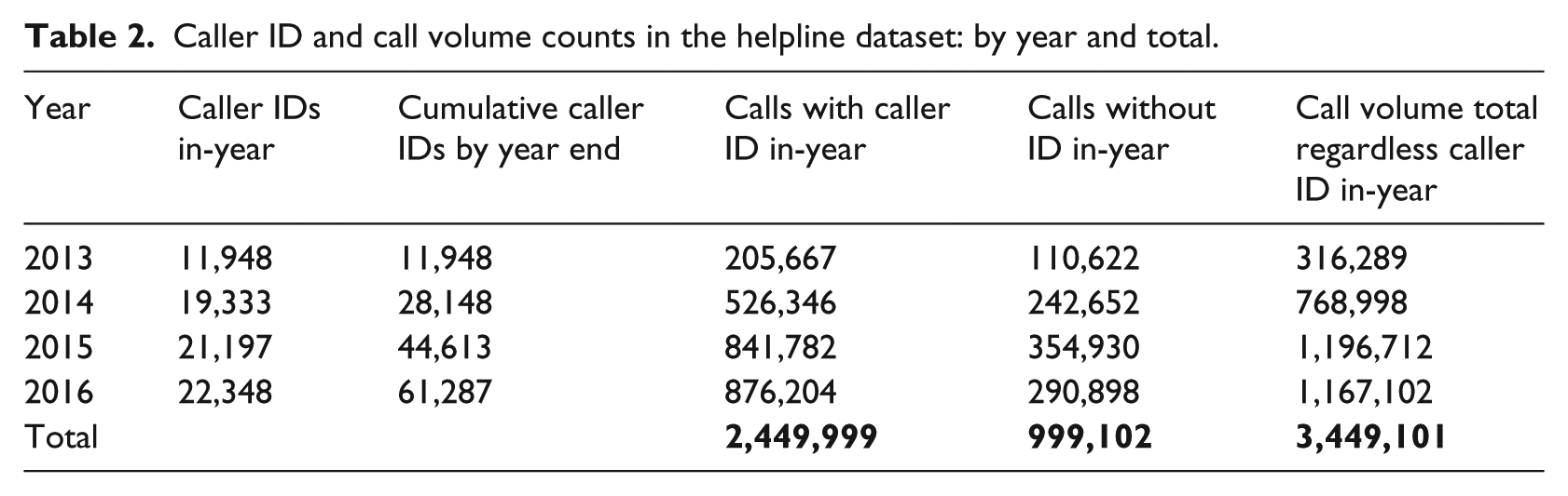
Notice that the straight sum of the in-year caller IDs in Table 2 exceeds the cumulative number of caller IDs in the dataset by year end 2016. This is because some callers contact the helpline across multiple years, and the telephony system remembers each caller ID forever.
Methods
Cluster analysis
Clustering involves grouping a set of objects (e.g. callers based on their attributes) in such a way that objects in the same group (called a cluster) are more similar to each other in comparison to other groups (clusters). Only the calls from callers with a unique identifier were used (44,613 callers collected in 2013–2015, increasing to 61,287 unique callers by the end of 2016). See Table 2 for more detail about unique caller IDs and call volumes associated with them.
Callers were clustered using three caller attributes:
Number of calls,
Mean call duration and
Standard deviation of call duration.
We selected these features due to their explanatory power: the number of calls a person makes indicates their frequency of help-seeking behaviour, the mean call duration indicates call length and the standard deviation of call durations indicates a person’s variability and consistency in conversation length.
From a machine learning perspective, these features provide the smallest and simplest possible feature set that captures both the magnitude and the variability information about the activity of an individual user, represented by a caller ID.
From an operational perspective, the number of calls associated with an individual caller ID contributes to the overall call volume that the helpline receives, while the individual call durations contribute to the overall airtime that the helpline needs to process calls. Knowing the structure of the caller population in terms of volumes and durations provides operational insight into the call centre workload.
In the 2013–2015 dataset, we found about 8000 callers who only called once. For such callers, the standard deviation of call duration was set to 0. We found ~1000 individual callers who never got through to a helpline volunteer, always receiving an engaged tone. For these callers, we set both the mean call duration and its standard deviation to 0.
Before running clustering algorithms on our data, we standardised the dataset: each of the three features was centred at zero and scaled to variance one.
We used the K-means clustering algorithm given it is the most widely used and established clustering algorithm in the unsupervised machine learning literature. The number of cluster centroids is a user-defined parameter. We used the heuristic elbow method, illustrated with Figure 1, which looks at the total within-cluster sum of squares as a function of the number of clusters. We then chose a number of clusters so that adding another cluster does not improve much better the total within-cluster sum of squares. Using this method, we discerned that five is a reasonably small number of clusters that would provide reasonable resolution in terms of explained variability.
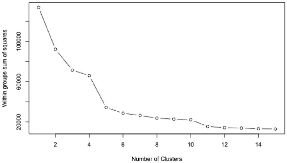
Elbow method illustration: the within-groups sum of squares sharply drops when we transition from four clusters to five and comparatively flattens out for all the higher numbers of clusters. This suggests K = 5 is the best number of clusters for the problem at hand, which incidentally is the 2013–2015 slice of our helpline dataset.
Throughout our clustering computations, statistical variability is measured in terms of sums-of-squares of the relevant deviations. With our choice of the three numerical clustering features, Euclidean distance was used as a natural measure of deviations. The total sum of squares was computed using the deviations of individual callers from the centroid of the whole dataset. The within-groups sum of squares is computed using the distance of an individual caller from the centroid of the assigned cluster. The between groups sum of squares uses the distances of cluster centroids from the dataset centroid and is numerically equal to the difference between the total sum of squares and the within-groups sum of squares.
The ‘explained variability’ reported in panels Figure 4(a) and (b) is the ratio of the between groups sum of squares to the total sum of squares. The unexplained variability is then the ratio of the within sum of squares to the total sum of squares. The plots shown in Figures 1 and 3, used in elbow method, can serve as charts depicting the change in slope of the unexplained variability with the increase of the number of clusters: consider the height of the curve at each K as the fraction of its height at K = 1 (leftmost dot on all elbow method plots).
The K-means clustering algorithm uses random sampling. The algorithm (implemented in R) outputs clusters as a numbered sequence, in order of extraction. This has an undesirable consequence: the order in which the clusters are extracted varies depending on which slice of the dataset is inspected. The same cluster can be listed under different numbers, making it difficult to identify across the years. To counter this effect, we consistently named clusters in tables and plots. We named each cluster using an index which consists of three decimal digits:
Digit 1: rank of the cluster against other clusters in terms of call duration. From short to long calls.
Digit 2: rank of the cluster in terms of number of calls, few to many.
Digit 3: rank of the cluster in terms of variability of duration, from smaller standard deviation to larger one.
For example, the clusters obtained in a five-cluster model, see Figure 4(a), were named as follows: 153, 221, 344, 435 and 512.
Periodicity analysis
Observations by the helpline personnel suggested that certain callers dial in at regular intervals. Thus, we set out to investigate whether cyclic patterns were present in the dataset. Using Fourier transform, we obtained the frequencies and the relative strengths of the periodic components of the call arrivals. Future work may involve transforming data in the frequency domain back into the time-domain allowing for call modelling and forecasting. However, in this first instance, our interest was to test whether periodic activity was present.
The point process of call arrival timestamps was converted into a time series. We split the time span into a large number of sampling intervals. We counted the number of calls arriving within each of these intervals. These counts became the values of our time series. The sampling interval (the bucket size for aggregating calls) was 30-min long, giving us the smallest number of sampling intervals at a resolution capable of capturing oscillations as frequent as once per hour. Our fundamental period, that is, the range of data supporting the analysis, lasted 2 years, or 24 months, or 731 days, or 17,544 h, or 30,588 sampling intervals exactly, or slightly over 104 weeks. The maximum meaningful frequency detectable at this resolution (Nyquist critical frequency, computed as half the sampling rate), equals 17,544 cycles over 2 years, or 731 cycles per month, or 24 cycles per day, or 1 cycle per hour exactly, or about 168 cycles per week.
To extract frequency components, we used a 2-year-long subset of the data from 01 January 2015 to 31 December 2016. Within this time span, the helpline call centre worked at full capacity. There were no structural changes that would drastically change either the capacity of demand for service, such as the opening of new branches or an introduction of free-phone access that took place in 2014. The call volume trend in 2015–2016 remained practically static, thereby the possibility of the trend masking some periodic activity remained low within this time span.
R programming language and R Studio were used for data wrangling and to implement the analysis. R libraries were used, namely, dplyr, readr, tibble, tidyr, scales and DescTools for wrangling, ggplot2 and DescTools for generating the visuals, fpc and cluster for clustering diagnostics, the base package stats provided routines for K-means clustering and Fourier transform.
Results
Descriptive analysis
The number of calls to the helpline had an increase each year but stabilised in 2015 and 2016. The proportion of repeat callers was high for each year (2013: 96.22%; 2014: 97.49%; 2015: 98.23%; 2016: 98.23%). The proportion of engaged calls increased each year (from 29.19% in 2014 to 48.21% in 2016).
The most popular time for calling is between 10 pm and 1 am for every day of the week (11 pm being the most popular hour). This is stable as there is a strong correlation between volume of calls per hour in 2015 and 2016 (r = 0.99 (confidence interval, CI = 0.98, 0.99), p < 0.0001). There was a number of peaks in call volume throughout the year (2013 peaked in May and August, 2014 peaked in August and December, 2015 peaked in August, 2016 peaked in June, October and December).
Average call duration in the dataset is 490 ± 819 s (8.17 mins). Average call duration increases from Monday to Friday and drops on Saturdays and peaks again on Sundays. Mean call duration has decreased each year until 2015 (2015 and 2016 are similar) indicating operational efficiency or a decrease in dialog due to an increase in service demand. While call duration dropped from 2013 to 2015, the weekly pattern remains consistent.
Intriguingly, the monthly influx of new callers in each month of each year is stable, both in relative and absolute terms. In Figure 2(a), dark blue bars show the counts of new callers that initiated contact for the first time in a given month (isNew = TRUE). Light blue bars show the counts in that month of return callers (isNew = FALSE). The bar plot starts at April 2013 where all callers were regarded as new, then the plot stabilises to show a ratio of ~48 to ~52 per cent of new callers to known ones.
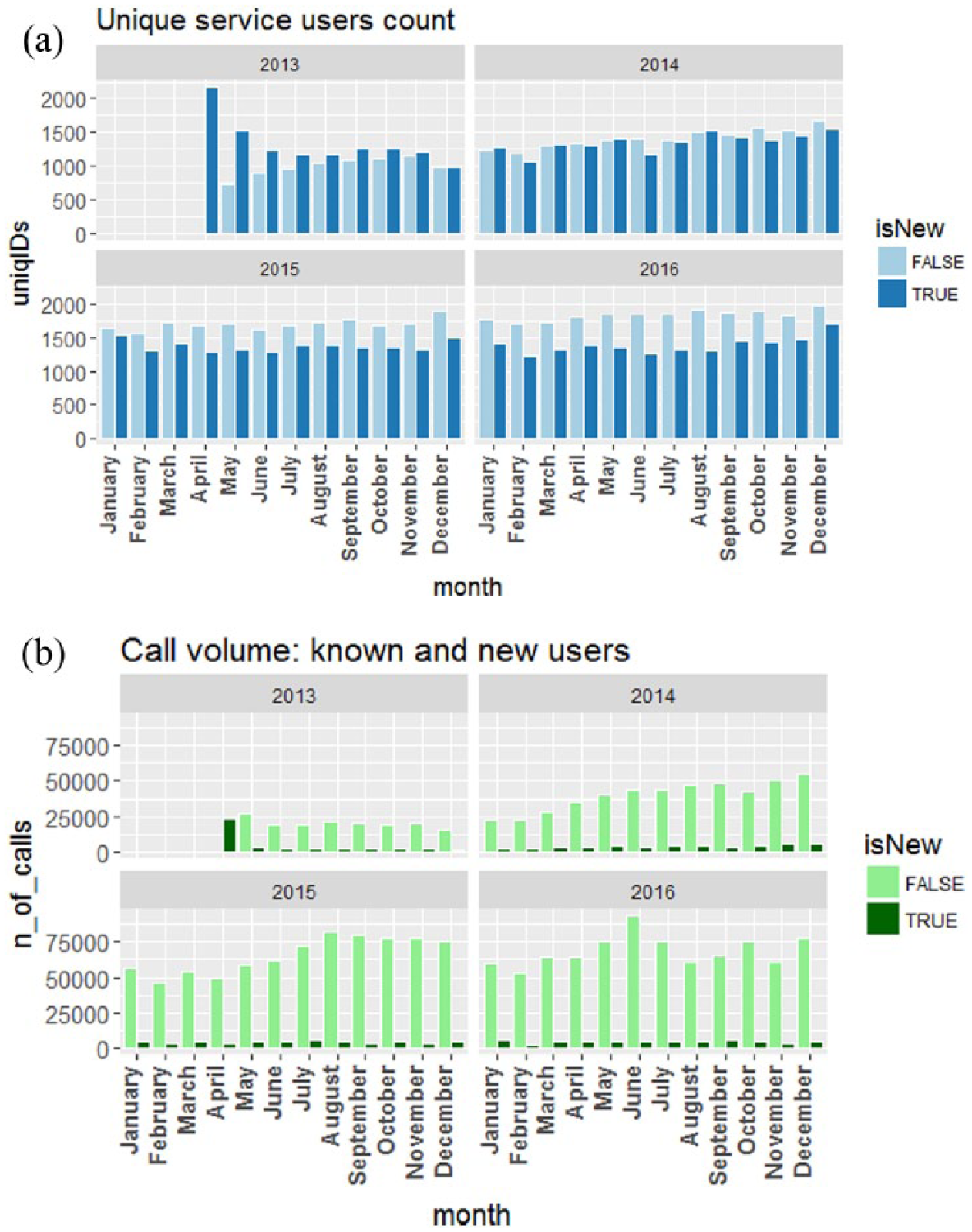
(a) Faceted monthly bar charts for unique service users count and (b) call volume for known and new callers. For every month, a caller either is new (isNew = TRUE) to the helpline, or has already been recorded in the dataset at some point in previous months.
Figure 2(a) implies that known callers eventually fade out. Had it not been so, the relative monthly share of new callers would have declined over time.
While ~50 per cent of callers in any given month is comprised of new callers, almost all of the call volume (i.e. the number of calls) in that month is generated by known repeat callers. In Figure 2(b), new callers (dark green) make up a small fraction of the call volume.
Clusters
The elbow method applied for various time slices of the helpline dataset, illustrated in Figure 3, most often delivered K = 5 as the best number of clusters. A six-cluster solution provided a reasonable alternative. Both of these solutions are discussed in detail below.
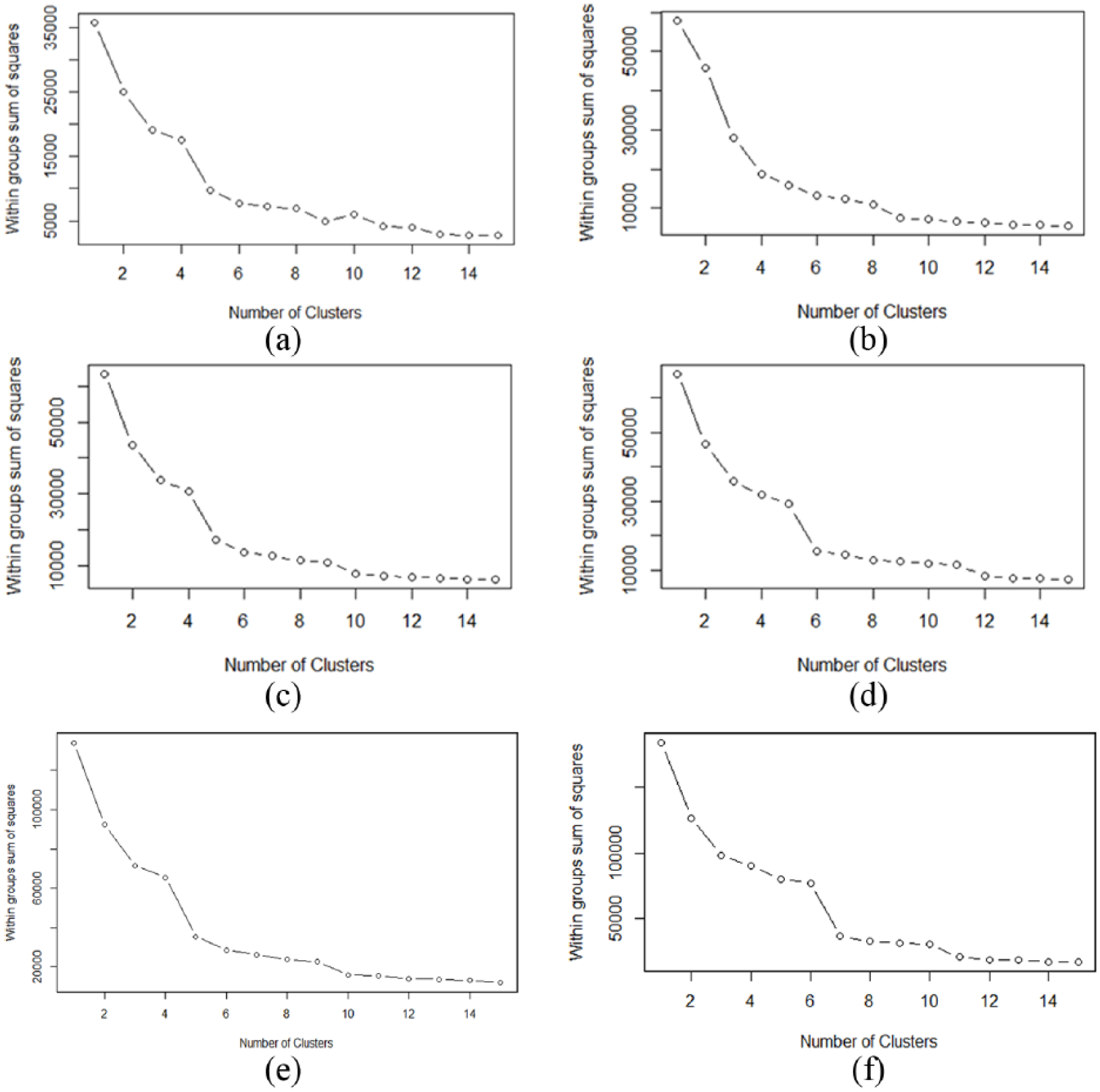
Elbow method results for various slices of the helpline dataset. Best K values discerned from these plots are (a) five, (b) undetermined, (c) five, (d) six, (e) five and (f) seven.
Figure 4 shows the clusters (types of callers) and their features. The meaning of the headings in Figure 4(a) and (c) are as follow:
name: three-digit name of the cluster: its index defined in the ‘Methods’ section.
volume: in-cluster mean of the number of calls made from each caller within that cluster.
mean: in-cluster mean of the personal mean duration (seconds) of calls within that cluster.
SD: in-cluster mean of the standard deviation of call durations (seconds) from callers in that cluster.
size: cluster size – number of callers captured in the cluster.
within SS: sum of squares characterising the dissimilarity of callers captured within this cluster. The smaller this number, then the more homogeneity is exhibited in the cluster.
Figure 4(a) and (c) show cluster properties in their original scales, while the clustering itself was performed with standardised data. Figure 4(b) and (d) display relative positions and shapes of clusters in standardised scales.
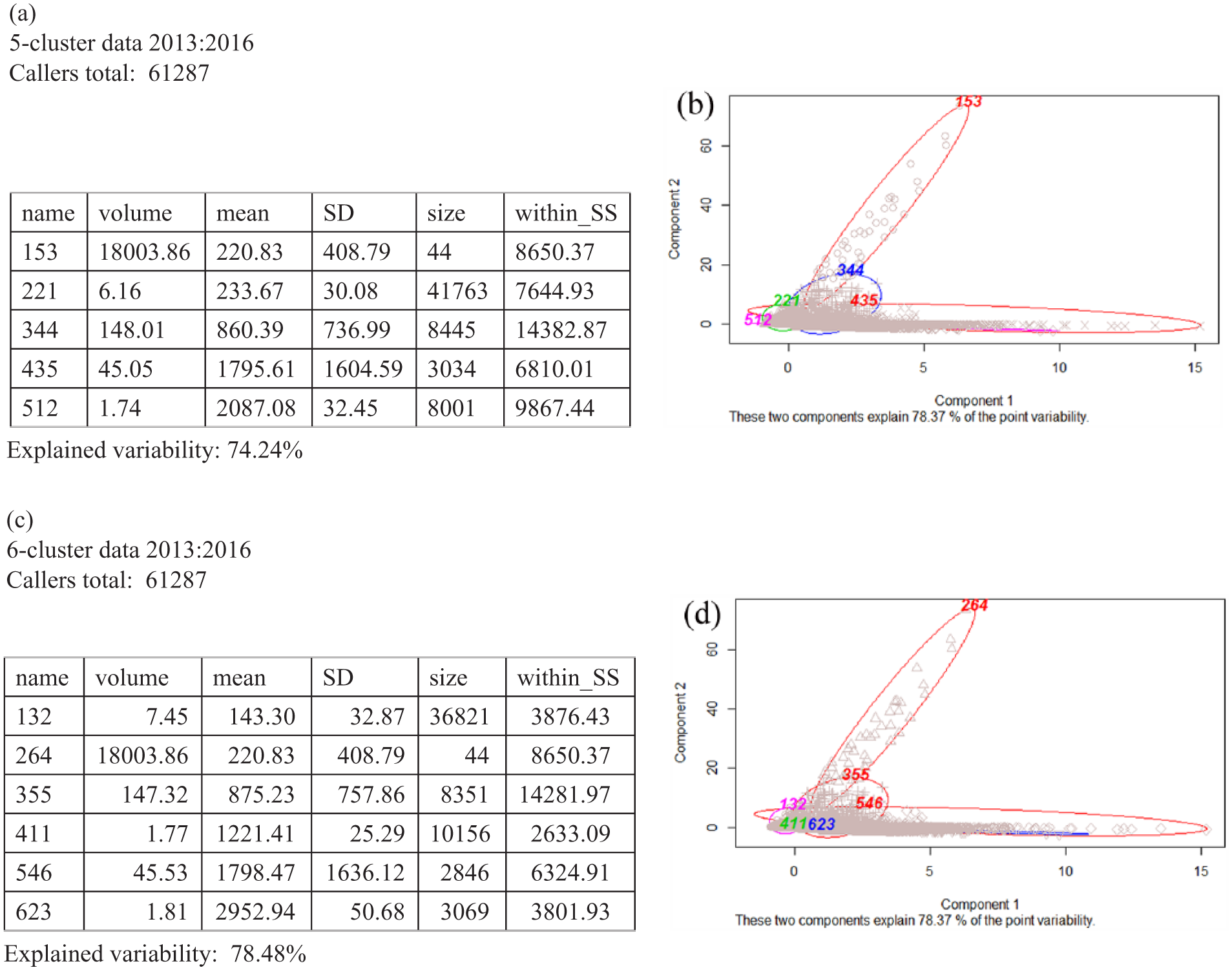
Clustering results. Panels (a) and (b) show five-cluster split, panels (c) and (d) show six-cluster split. Tables (a) and (c) show cluster averages for each of the three features: call volume, call duration, standard deviation of call duration, as well as cluster sizes and the values of the within-cluster sums of squares. Plots (b) and (d) show a projection from the feature space onto the plane of two principal components.
Five cluster solution
We interpreted the five clusters shown in Figure 4(a) as follows:
Cluster 153 (Elite prolific callers): the largest average number of calls per caller in the cluster and the smallest cluster size. A handful (less than 50 callers over the 4-year time span) of extremely prolific callers, responsible for 20 per cent of the total call volume. They call thousands of times, each call on average lasts about 4 min, with a small minority of calls lasting 10 min.
Cluster 221 (Typical callers): the largest cluster size. The majority of callers who call five to six times and almost always have a short 3- to 4-min conversation each time. This cluster accumulates 40–50 per cent of all callers depending on the time slice under consideration.
Cluster 344 (Standard prolific callers): second largest average number of calls per caller, middling average call duration and the largest unexplained variability encompassed by the cluster. About 12–15 per cent of callers are prolific, each calling hundreds of times and having call durations that are moderate in length (from a few minutes to half an hour long).
Cluster 435 (Unpredictable erratic callers): the largest average standard deviation of the call duration. About 3–5 per cent of callers whose call duration varies considerably, with some calls lasting 3 min and some up to 1 h.
Cluster 512 (One-off chatty callers): the smallest average number of calls per caller accompanied by the largest average call duration. About 13 per cent of callers who only call one to two times have a long 30-min to 1-h conversation and do not return for any sustained support. The operational opposite to prolific callers.
The three-digit cluster names shown on the principal components visualisation Figure 4(b) and (d) are the same as the three-digit cluster names shown in the tables in Figure 4(a) and (c), respectively. Principal component axes form a plane in the feature space orientated such that the projection of the dataset onto this plane shows the widest possible two-dimensional footprint of the dataset. The feature space in this case is three-dimensional since we cluster with the values of volume, mean and SD.
The five-cluster split was first done for the 2013–2015 time span. Clustering was then re-run using the 2016 dataset. The five clusters emerged from both datasets. We also re-run the clustering for each of the years 2013, 2014, 2015 and 2016 separately. Despite the different sizes and time spans, the prominent features of the identified clusters remained invariant. The graphical images of the clusters in terms of the principal components retained their visual features, such as the shape and relative position in the feature space of each cluster. For example, the Elite Prolific cluster in each case produced a shape that dictated the direction of the second principal components axis (refer to the image of cluster 153 in plot Figure 4(b)).
Six-cluster solution
As clustering uses human judgement to input the number of clusters to seek out, we decided to try detecting six clusters instead of five. Computations showed that the One-off Chatty cluster splits into two sub-clusters, Figure 4(c) and (d). We found that four out of five clusters previously identified using the five-cluster model survived. Elite Prolific callers (cluster 264) in Figure 4(c) remained intact, compared with cluster 153 in Figure 4(a). The Typical, Standard Prolific and Unpredictable clusters, named 132, 355 and 546 in Figure 4(c), also retained their characteristics. However, the One-off Chatters cluster was divided into two new clusters:
Cluster 623 (Long-haul one-off) – the callers who command the longest average call time;
Cluster 411 (Typical one-off) – the second largest of the six clusters. This new cluster is ‘typical’ because its SD is of the same order of magnitude as that of the Typical callers (cluster 132) rather than that of Standard Prolific callers (cluster 355).
The six-cluster picture from both summary tables and principal component plots remained stable for all time slices considered: 2013:2015, 2013:2016 and every separate year 2013–2016. Overall, the explained variability of the six-cluster model only marginally increased in comparison to the five-cluster model. Figure 5 shows boxplots for each of the three features of each cluster.
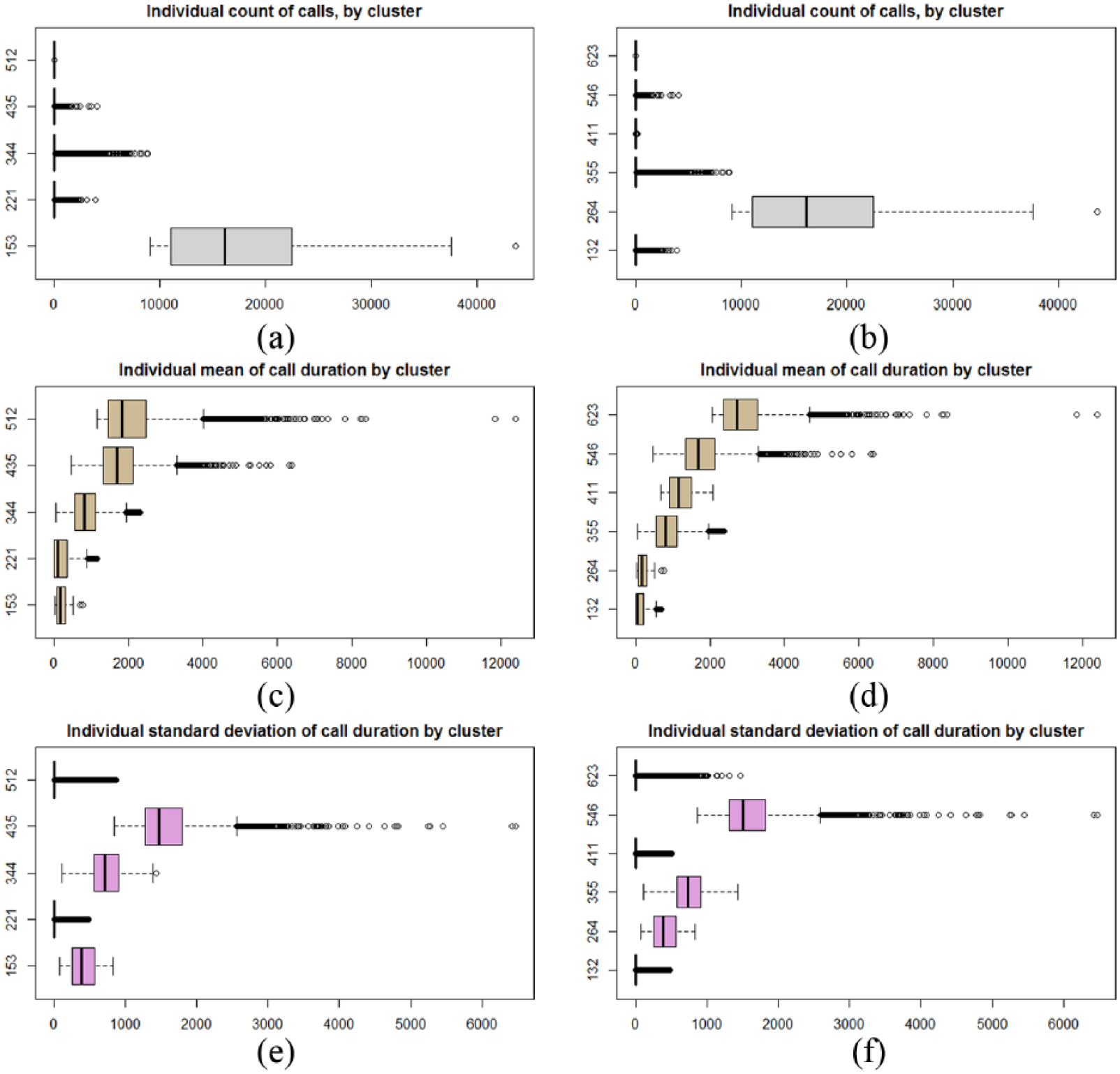
Boxplots revealing the cluster medians, the interquartile ranges and the total ranges for each of the clustering features. Panels (a), (c) and (e) show five-cluster split. Panels (b), (d) and (f) show six-cluster split: (a) five-cluster, volume count; (b) six-cluster, volume count; (c) five-cluster, mean in seconds; (d) six-cluster, mean in seconds; (e) five-cluster, SD in seconds and (f) six-cluster, SD in seconds.
Other solutions summary
We experimented with both fewer and more clusters. A three-cluster solution yielded a substantial reduction of the explained variability: ~54 per cent with three clusters versus ~74 per cent with five clusters. Attempts to build a solution with 7–11 clusters exacerbated the issues in explaining the ever finer distinctions between clusters, whereas the explained variability of the data increased only moderately, remaining between 80 and 86 per cent. The Elite Prolific cluster remained very stable throughout, and the largest Typical cluster remained over 3.5 times as large as the second largest cluster. Overall, the five-cluster and the six-cluster models provide the most insight and are easily interpretable.
Call duration
The statistical distribution of answered call durations provided a number of new insights. The call duration distributions plotted on a linear scale turned out not to be very informative. The empirical density curve resembled a negative exponential. However, attempts to fit a log-normal or gamma distribution showed a poor fit.
At a first glance, the duration of calls appears to follow an exponential decay distribution, where the volume of calls decreases at a rate proportional to call duration. However, the distribution follows a complicated decay pattern with a rate that associates with the call duration in a non-obvious manner.
If the time is measured on the logarithmic scale with base 60 s, then the 1-min time point is plotted at position 1.0, 1 h (3600 = 60 × 60 s) plots at position 2.0 and so on. Using this scale, the distribution of call durations can be seen in Figure 6(a) for all callers and in Figure 6(b) for Elite Prolific callers only.
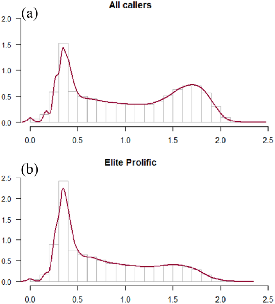
(a) Call duration distribution of all callers and (b) call duration distribution, Elite Prolific cluster. On both panels, the abscissa shows the logarithm of duration. The logarithm is taken with the base 60 s. The ordinate shows the probability density values.
The logarithmic bimodal structure of call durations is evident in Figure 6(a). The left peak denotes snap calls: position 0.5 on the logarithmic scale corresponds to about 10 s linear time. The volunteers with the helpline developed knowledge and understanding of the ‘snap’ calls, typically a few seconds long, normally silent, which corresponds to the 10-s peak. The right peak between positions 1.5 and 2.0 (10 min and 2 h) denotes longer conversations. The almost straight interval in the middle of the distribution corresponds to an exponential decay (but not quite).
A common approach to model call durations found in literature recommends removing ‘too short’ calls from a dataset and model the ‘main body’ of the calls using a log-normal distribution. 10 This approach is undesirable in our case. Helplines are particularly interested in describing, and ultimately predicting, the short and snappy call patterns. For example, most calls from Elite Prolific callers are snappy: not exceeding 10 s (position about 0.5 on the horizontal axis), Figure 6(b). A removal of ‘too short’ calls would have removed this influential cluster of callers from view.
Frequencies
Figure 7 depicts spectral plots of the Fourier transform as described in the methods. The frequencies of oscillations are plotted against the amplitudes that measure the peak number of calls.
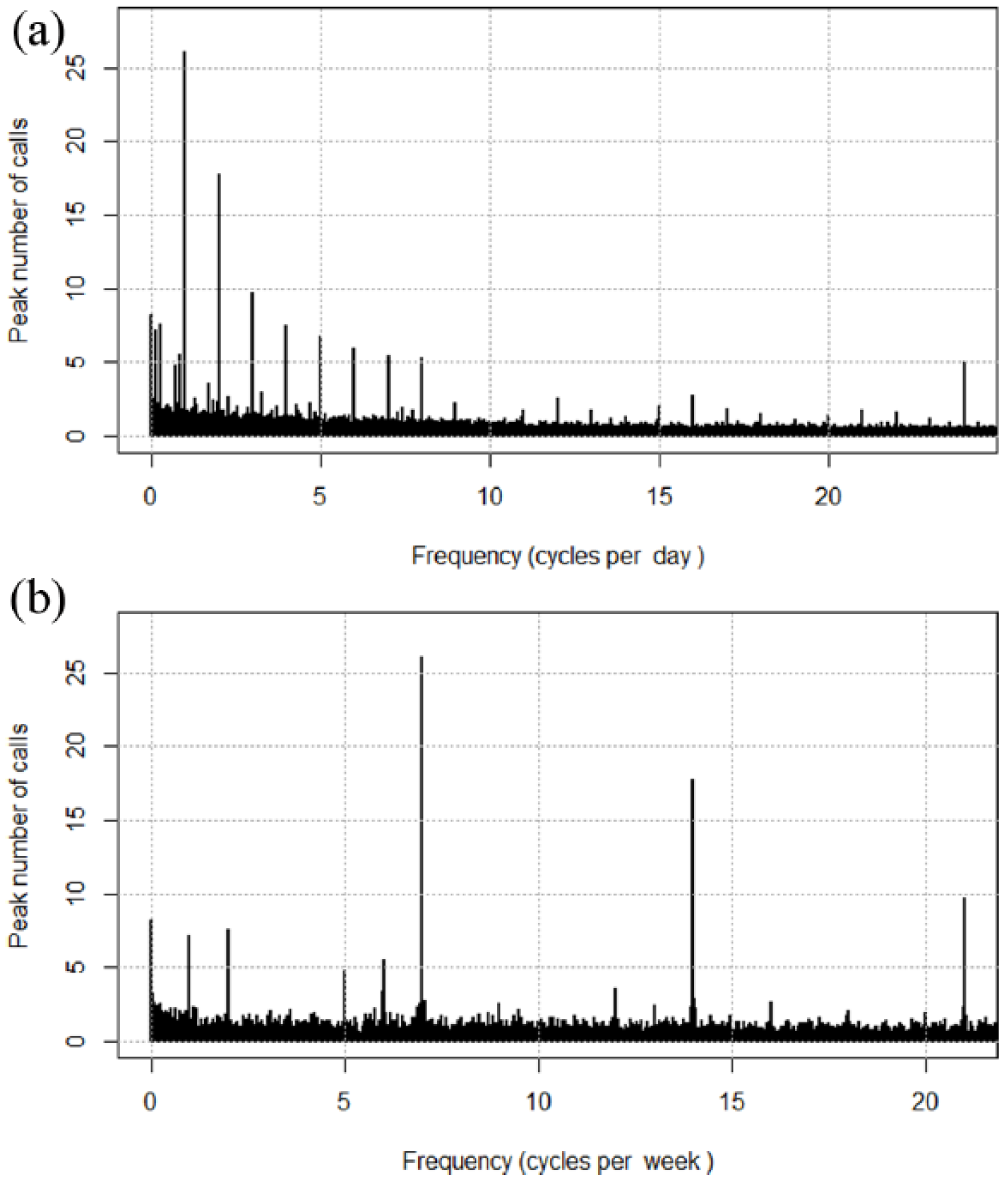
Spectral plots: (a) for the whole dataset and complete frequency range and (b) for the whole dataset, showing the lowest 1/8 of the frequency range; here frequencies are expressed in cycles per week.
We found a strong intra-day oscillation pattern and a secondary intra-week oscillation pattern. These oscillation patterns, first observed in the overall dataset, persist through both the cluster of Elite Prolific callers taken separately and the remainder of the dataset (i.e. everyone except the Elite Prolific callers).
The spectral plots are shown after de-trending that amounted to removing the non-oscillatory component which would have shown as frequency of 0 cycles.
The strongest set of dominant frequencies corresponds to intra-day oscillations, at 1, 2, 3, 4, 5, 6, 7, 8 and 24 cycles per day, Figure 7(a). The 24 cycles per day frequency sits at the limit of our resolution (Nyquist frequency, see ‘Periodicity Analysis’ in ‘Methods’ section). On the left of Figure 7(a), at the frequency range between 0 and 1 cycles per day, there is a secondary group of frequencies.
Figure 7(b) depicts a closer view of this secondary group of frequencies, expressed using cycles per week. On this plot, the secondary group of frequencies, associated with intra-week oscillations, is clearly seen. These secondary dominant frequencies are situated at 1, 2, 5 and 6 cycles per week. Their amplitudes range from five to eight calls. These frequencies correspond to a natural human inclination to repeat tasks weekly, or twice weekly, or every working day, or every day except Sunday (or another special day of the week). The large amplitude at 7 cycles per week shows exactly the same oscillation as the once-a-day amplitude in Figure 7(a).
Further to the right on the plot in Figure 7(b), the 12 cycles a week frequency can be visually set apart from the noise. However, its strength amounts to about 3.5 calls only, which is between 2 and 2.5 times inferior to the weakest of the previously identified dominant frequencies. Therefore, we do not include weaker frequencies in any of the two identified groups of frequencies.
The prominent amplitude of eight calls, visually shown at near 0 cycles per week on the plot Figure 7(b) is actually situated at 0.2 cycles per month or about twice a year. Other frequencies from monthly and quarterly ranges, corresponding to less than 1 cycle per week, are lacking prominence.
Discussion
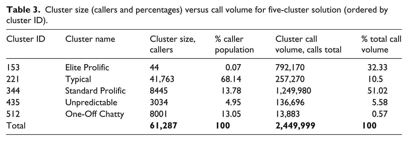
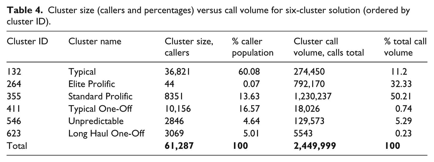
Our observed lack of fluctuation of a monthly new caller influx as shown in Figure 2 implies that people turn to the helpline mostly for endogenous reasons, such as ongoing mental health issues and social isolation, described earlier, from the literature. Exogenous reasons, such as natural seasons, economic turmoil or media stories and promotion campaigns appear to bear little weight on people’s decisions to initiate contact for the first time. It remains to be seen how these factors affect the patterns of behaviour of existing callers. Tables 3 and 4 provide some summary detail on cluster size (callers and percentages) versus call volume for five- and six-cluster results.
Cluster size (callers and percentages) versus call volume for five-cluster solution (ordered by cluster ID).
Cluster size (callers and percentages) versus call volume for six-cluster solution (ordered by cluster ID).
The volume of calls exhibits strong intra-day and intra-week repetitive patterns, while intra-month repetitions are conspicuously absent, as discussed in the ‘Frequencies’ section of ‘Results’. This double periodicity effect is well known in a call centre context.11,12 The once-an-hour, or 24 cycles per day, frequency was part of our intra-day periodicity pattern. As this frequency sits right at the limit of our current resolution, it would be worthwhile re-sampling the time series of calls at a higher rate, for example, with 5-min time buckets, and re-running the frequency analysis to see if any higher frequencies contribute to the pattern.
Further work is needed to estimate how prevalent the bimodal or multi-modal statistical distributions of call log-durations are on the individual caller level. Multiple modes would indicate that a caller is talking to the helpline for support through different periods of crises. In order to model the behaviour of these callers successfully, the helpline call data recording protocols would need to be revised to include in the dataset a flag indicating the main reason for the call. A consensus opinion in statistics maintains that a multi-modal distribution strongly suggests a stratified underlying population: detecting and separating these strata remains future work.
Conclusion
This work presented an analysis of 3.5 million calls made to a mental health and well-being helpline, seeking to answer the research question, ‘What different groups of callers can be characterised by specific usage patterns?’ A related research question was, ‘If identified, then do such groups of usage patterns change over time?’
The results show that different groups of callers can be identified by their collective usage patterns. Unsupervised learning using K-means clustering identified five clusters, namely, Elite prolific callers (largest average number of calls per caller in the cluster and the smallest cluster size), Typical callers (the largest cluster size), Standard prolific callers (second largest average number of calls per caller, Unpredictable erratic callers (largest average standard deviation of the call duration) and One-off chatty callers (smallest average number of calls per caller accompanied by the largest average call duration). Details on these clusters are presented in the ‘Clusters’ section of ‘Results’. Furthermore, the identified groups of usage patterns are stable and re-emerge regardless of which year is considered.
The most striking of those clusters, that we termed Elite Prolific callers, encompasses a small number of caller IDs responsible for a substantial share of the total call volume that the helpline receives. Early identification of callers of this type and routing their calls to specialized helpline volunteers provide insights in the modelling of healthcare service usage, offering actionable intelligence for evidence-based practice and operational decision-making. Our work in this area has shown promising results. 13
This work shows that one can model the different types of service users (callers) and the complex nature of caller behaviour and patterns to optimise resource management, volunteer productivity and forecast demand. This analysis offers an opportunity to review the skillset and training needed by volunteers to best support service users. Matching skillsets and training to caller needs serves to improve job satisfaction and productivity.
Footnotes
Declaration of conflicting interests
The author(s) declared no potential conflicts of interest with respect to the research, authorship and/or publication of this article.
Funding
The author(s) disclosed receipt of the following financial support for the research, authorship and/or publication of this article: Financial support for this study was provided in part by Samaritans Ireland together with Ireland’s National Office for Suicide Prevention. The funding agreement ensured the authors’ independence in designing the study, interpreting the data, writing and publishing the report.