Sage Journals: Discover world-class research

Abstract

An empirical correlation and a set of machine learning (ML) models were developed to estimate droplet size and count distributions over an extended duration after a cough at different relative humidities (RHs), air temperatures and locations within an indoor environment. Experiments covered RHs of 20%–80% and air temperatures of 21 °C–26 °C. Droplet count distributions for 4 size bins (0.3–0.5, 0.5–1, 1–3 and 3–5 μm) were recorded for 70 min within the distance of 2 m from the cough source. Different ML models, including decision tree, random forest and artificial neural network, were trained for each size bin to predict the associated count distribution. Amongst these models, random forest showed a slight superiority in performance. The coefficient of determination for the random forest models ranged from 0.912 to 0.989, indicating robust correlations between the features and the response variables. An empirical correlation was established linking the count distribution of 0.3–0.5 μm droplets to time, RH and distance along the cough direction. Both ML models and the correlation accurately predicted the trends and the distributions, providing valuable data for validating computational simulations and informing indoor environment control systems to reduce the risk of virus transmission.

Keywords

Cough Aerosol Size distribution Relative humidity Prolonged period Machine learning

Introduction

The COVID-19 pandemic has proven that understanding the exact transmission routes of airborne diseases is extremely important to limit the spread of infectious pathogens. Viruses like these are carried in respiratory droplets with diameters ranging from 0.2 μm to several hundred microns and can be transmitted via exposure to environmental fomites, close contact with virus-carrying droplets, and/or aerosol transmission.^1–7 The latest mechanism is known as inhalation of very small droplets (generally droplets smaller than 5 μm).^1–7 Various studies show that the SARS-CoV-2 virus can remain active in aerosols for several hours, with longevity influenced by factors such as droplet size distribution, ultraviolet (UV) index, air temperature and relative humidity (RH).^1,8–13 Other variables, such as human physiology, the utilization of face coverings, the proximity of people, airflow properties within a given space and ventilation strategies, can also affect aerosol transmission of disease.^14–21 Understanding the influence of these factors is crucial for developing effective strategies to control the spread of infectious pathogens.

Several numerical and experimental studies have been conducted to understand the effects of indoor environmental factors, such as air temperature and RH, as well as time and distance, on the lifetime and dispersion of cough-generated droplets and aerosols.^{1,2,8,22–37} Dabisch et al.⁸ used a rotating drum aerosol chamber to investigate the influence of temperature, sunlight and RH on the lifetime of SARS-CoV-2 in droplets. By injecting fine droplets with a mass median aerodynamic diameter (MMAD) of 2 μm into the chamber and measuring the virus concentration, they found that the time required for a 90% reduction in infectious virus ranged from a few minutes to over 2 hours, depending on environmental conditions. However, the authors noted that their findings were limited to a single droplet size distribution and that droplet size has a significant influence on the results.

Chong et al.²⁵ used direct numerical simulations to investigate the effects of RH on the lifetime of respiratory droplets. They found that increasing the ambient RH significantly prolonged the lifetime of droplets and aerosols, mainly due to the effects of humidity on droplet evaporation. It was demonstrated that the extension of the droplet lifetime with humidity is so pronounced that 10 μm droplets rarely evaporated and were carried in an aerosolized way. This result contradicts the World Health Organization’s classification (WHO),¹⁸ which indicates that droplets with a diameter greater than 5–10 μm fall ballistically to the ground. Chong et al.²⁵ also showed that as droplet size decreases, its lifetime increases, and it travels a longer distance from the cough source. This finding was consistent with previous experimental results.¹

Zhao et al.²⁴ investigated the influence of ambient temperature and humidity on the lifetime and trajectory of respiratory droplets produced by speech. They considered a wide range of temperatures (0−40°C) and RH (0−92%) and found that droplets can travel farther downstream in low-temperature and high-humidity conditions, while the number density of droplets increases in high-temperature and low-humidity environments. Mesgarpour et al.^32,33 studied the effects of ambient conditions on the spatio-temporal distributions of exhaled droplets in a bus. They demonstrated that a 10% increase in RH caused a 30% increase in droplet concentration at the farthest point from a coughing passenger. Trivedi et al.³⁷ also assessed the size and position distributions of droplets after a cough in room conditions at 20°C and 40% RH. After analysing 10 independent coughs, they showed that although turbulence intensity decreases far from the coughing person, significant changes in the position distributions of the droplets can still be observed.

In a previous study,¹ the present authors experimentally investigated the spatial and temporal dispersion of cough-emitted droplets over a long duration (70 min) at various locations in front of- and behind the cough source. The experiments were performed under ambient conditions on several days where the air temperature and RH were in the range of 21°C–26°C and 20%–78%, respectively. In this case, the effects of initial droplet size distribution, RH, air temperature, distance from the cough source and time on the dispersion of droplets were taken into account. Our findings showed that aerosols with sizes ranging from 0.3 to 10 µm persisted for a long time in a still environment. After 70 min, about 20% of the maximum nuclei counts were found to be almost uniformly distributed in the sealed enclosure. Furthermore, it was numerically demonstrated that an increase in ambient temperature led to a decrease in both droplet counts and average diameter. In addition, increasing RH resulted in an enhancement of the number density of suspended droplets.

Most studies in this field primarily focus on the in-flight behaviour of cough-generated droplets and aerosols for only a few seconds after the cough. Particularly for numerical simulations, the computational expense of tracking thousands of particles for 1–2 h in a room is onerous. As a result, in the previous paper (similar to other numerical works),¹ droplet in-flight behaviour was simulated for only 6 s after the cough. However, as stated above, small droplets can remain suspended in the air for several hours, potentially carrying active virus. Therefore, to better understand the transmission of respiratory viruses over long periods, more analytical, experimental and machine learning (ML) studies are needed.

Over recent years, ML models have found widespread application in detecting COVID-19 through various means, including voice, cough, breathing patterns, X-ray and CT images (often addressing classification problems).^38–40 The ML models have also been integrated with computational fluid dynamics (CFD) simulations to predict the spread of respiratory droplets under different conditions, such as in public transport.^{32,33,41–43} Nevertheless, the complexity of collecting experimental data has led to a notable scarcity of studies focusing specifically on the development of ML models based on experimental results for predicting the spread patterns of respiratory droplets. In a study by Liu et al. ⁴⁴ a series of machine learning (ML) models were developed using experimental data to forecast the concentrations of exhaled aerosol exposure amongst healthcare workers in an operating room. The focus of their investigation was specifically on breathing patterns, enabling them to anticipate aerosol concentrations in six different locations within the healthcare workers' breathing zones. The study highlighted the potential utility of machine learning in predicting aerosol concentrations. However, the challenge arises as a specific model was recommended for each location, making it difficult to extrapolate predictions to locations not covered in their experimental measurements. Additionally, the study did not consider the impact of time and was confined to PM_0.3 concentrations exclusively. Moreover, ML models have been applied to analyse the effects of environmental factors on disease transmission at broader scales, such as in cities. In a study conducted by Hariharan,⁴⁵ the impact of daily mean temperature, absolute humidity and average wind speed on the attack rate and mortality rate of COVID-19 in Delhi, India, was investigated. The study utilized a random forest algorithm to compare epidemiological and meteorological parameters. Notably, it was found that absolute humidity is the most influential variable for both the attack rate and mortality rate in the analysis.

The objective of the current study is to develop an ML model and an empirical correlation to estimate the size and count distributions of cough-generated droplets over a long duration in a still environment at different air temperatures, RHs and locations. In a comprehensive review article, Wang et al.² analysed the literature regarding the transmission of respiratory viruses by aerosols and it was revealed that for most respiratory activities, such as breathing, speaking and coughing, most exhaled aerosols are smaller than 5 μm, and a significant portion is less than 1 μm. Moreover, studies have indicated that viruses are abundant in small aerosols (<5 μm). Therefore, the current study was focused on droplets smaller than 5 μm.

Methodology

Collecting data from experiments

Over a 7-month period, 55 experiments were conducted at Toronto Metropolitan University across several days to investigate the spatial and temporal dispersion of aerosol droplets under various environmental conditions and to forecast their behaviour for prolonged periods (i.e. more than 1 h). In these experiments, which were conducted in real conditions, the air temperature ranged from 21.9 to 25.8°C and the RH varied from 20% to 78%. The experimental setup and droplet count measurements for different size bins were thoroughly described in our previous paper¹; therefore, only a summary of the experimental methodology and measurement data is given here.

Experimental setup

An artificial cough generator was designed to simulate respiratory activity with droplets. It comprised two parallel pressurized air flow lines, respective flow controllers for calibrating air flow rates, solenoid and manual valves to control the flow duration, an aerosol/droplet generator to produce desired size distribution (using a Laskin-type nozzle), an HEPA filter to remove any dust and particles from the flow, a control box and a digital delay generator for synchronizing the cough with a camera and laser/LED-based lighting system, and a manikin to release the droplet-laden flow (a section of the setup is shown in Figure 1-(a)). By atomizing a solution of propylene glycol, small droplets were generated with diameters less than 10 μm (since the surface tension of propylene glycol is less than that of water) and the droplet size distribution fell within the range of interest. For this study, the cough flow rate and the average velocity at the manikin mouth were 3 m³/h and 4.8 m/s, respectively.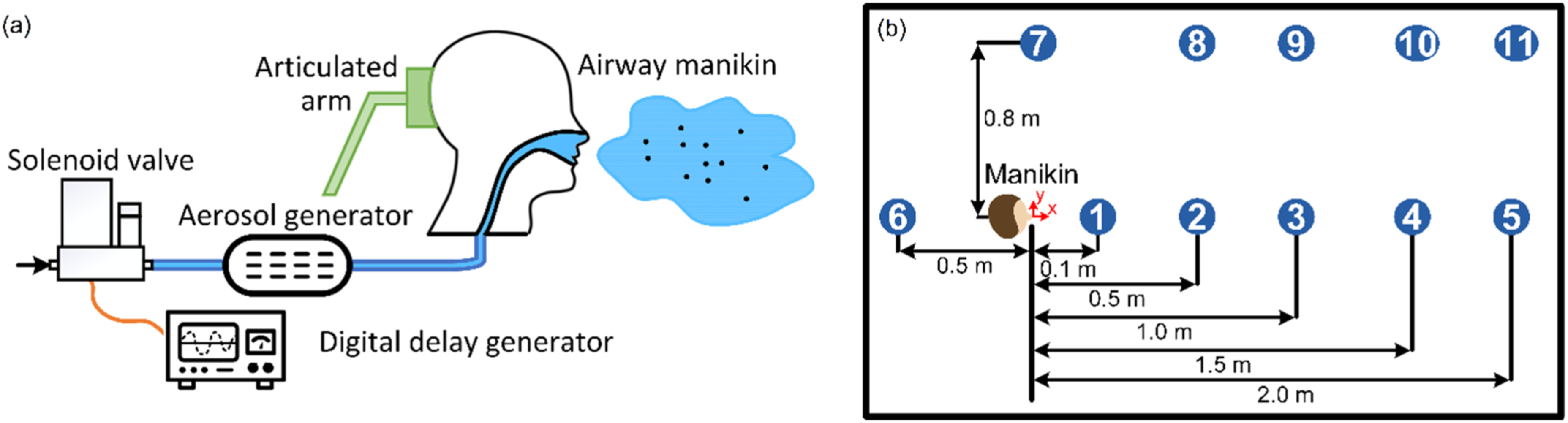

Figure 1.

(a) Schematic of the artificial cough generator and the control system¹; (b) A schematic of the measurement locations inside the sealed enclosure.¹.

The experiments were carried out inside a sealed enclosure with dimensions of 2.5 m in length, 1.6 m in width and 1.9 m in height. The manikin’s mouth was set at a height of 1 m. As shown in Figure 1-(b), which depicts a top view of the chamber layout, 11 locations were selected to measure droplet count and size. The first five locations were arranged in the direction of the manikin’s cough, the sixth location was positioned behind the manikin, while locations seven through 11 were set 0.8 m to the side of the manikin’s mouth.

Experimental measurements and data structure

A commercial droplet counter (Kanomax brand) was used to collect samples from these 11 locations, measuring droplet number density in six bin sizes ranging from 0.3 to 10.0+ μm. The droplet counter was programmed to collect data at 7-s intervals for each location, with a total sampling time of 70 min. The experiments were repeated five times for each location.

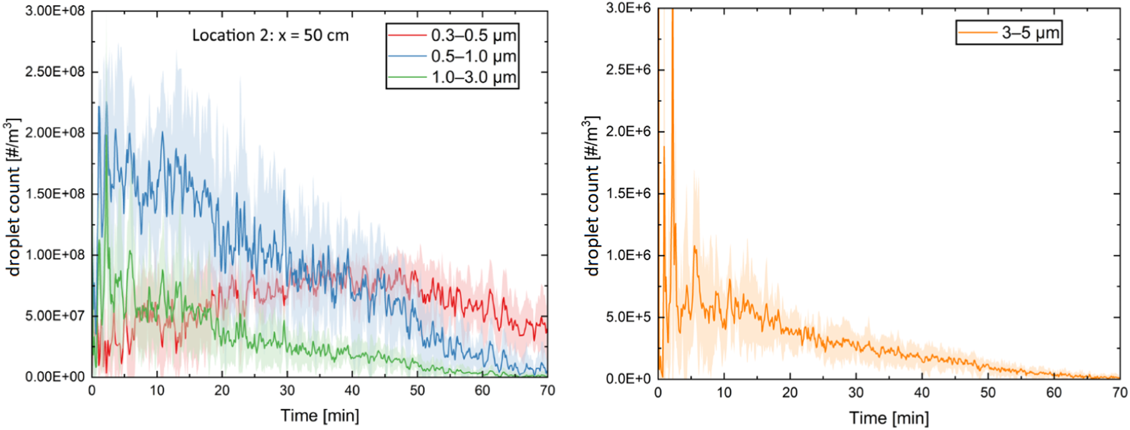
Figure 2 shows the variations in droplet count over time at location 2 for the size bins of 0.3–0.5, 0.5–1.0, 1.0–3.0 and 3.0–5.0 μm.¹ The shaded region in this figure represents the standard deviation of the average over five measurements. It is clear from the highly variable nature of the curves that turbulence and droplet diffusion have a significant impact on droplet count. Moreover, in certain cases, such as 3–5 µm, noticeable spikes can be seen, which are attributed to the bulk transport of the droplet plume after coughing.¹ For additional details on the forecast and experimental results (e.g. droplet count at other locations), readers are referred to the previous study.¹ The rationale behind placing Figure 2 in this section is to showcase the output data and its structure before delving into the explanation of ML approaches and results. It aligns with common practices in machine learning studies, in which providing an overview of the data helps readers understand the nature of the information being processed.

Figure 2.

Droplet count measured at 0.5 m in front of the cough source (location (2)) for four size bins. The shaded area shows the standard deviation of the averaged results over five measurements.¹

Moreover, it is crucial to highlight that the distribution of droplet sizes and counts in our research aligns with results reported in existing literature. Gralton et al.,⁴⁶ in a review of 26 studies, revealed that particle sizes generated during activities like breathing, coughing, sneezing and talking by healthy individuals ranged between 0.01 and 500 μm, while individuals with infections produced particles in the size range of 0.05 to 500 μm. Additionally, in the study by Liu and Novoselac,⁴⁷ which explored the spread of a simulated cough, particle trajectories for sizes of 0.77, 2.5 and 7 µm were observed, with results indicating that 0.77 µm particles remained entirely suspended. Furthermore, the reported droplet concentration in our work aligns with the outcomes of Lee et al.⁴⁸ and Yang et al.¹⁵ Lee et al.⁴⁸ discussed that the number of particles expelled per cough when subjects had a cold ranged from 731,000 to 18,756,000. They also reported that most particles generated by coughing are small enough to be suspended in the air, and they found that patients with a cold can release airborne transmission-available particles, with transmission detected at a distance of 3 m. The values of droplet concentrations reported in the work of Yang et al.¹⁵ are in the same order of magnitude as our data.

Complexity in interpretation of experimental results and necessity of developing machine learning models

Although the experimental study was conducted under real indoor conditions, the effects of RH and air temperature on the spatial and temporal dispersion of aerosol droplets cannot be determined precisely from the experimental data due to their overlapping influence.¹ For instance, it remains ambiguous how the dynamics of droplets and aerosols evolve over a long duration (70 min) if the RH varies from 30% to 60% while the air temperature remains constant. Similarly, predicting the spatial and temporal dispersion of aerosol droplets under a new set of conditions (for instance, when the air temperature and RH are 21°C and 40%, respectively) that were not experimentally tested is not straightforward. Numerical simulations were conducted in our previous study to understand the droplet in-air behaviour at various ambient temperatures and RHs.¹ However, the numerical simulations typically only show the droplet behaviour for a few seconds (typically less than 10 s), due to computational limitations.

To address the aforementioned issues and predict the in-flight behaviour of droplets over a prolonged period, ML models have been developed in this study. Specifically, a comprehensive and diverse dataset has been collected from the experimental study, which can be used to train an ML model and predict the temporal and spatial distributions of cough-generated droplet size and count under different RH and air temperature conditions over the course of an hour.

Developing machine learning models

In the present study, the concept of supervised learning was utilized to develop the ML models.⁴⁹ In this approach, the model learned from labelled examples or training data (where each example was a pair comprising an input vector and desired outputs) to accurately predict the outputs for unseen cases. The dataset obtained from 55 experimental measurements mentioned above (five measurements at each location (1–11)) under different air temperature and RH conditions was used to train the ML models. In the dataset, there were a total of 136,400 data points (rows). The inputs to the model include air temperature, RH, time, x and y distances (axial and orthogonal distances from the manikin’s mouth, respectively), while the output was the droplet count. Table 1 presents a statistical overview of the input data. As previously mentioned, this study focused on predicting the behaviour of droplets smaller than 5 μm. Four ML models have been developed for four size bins (0.3–0.5 μm, 0.5–1 μm, 1–3 μm and 3–5 μm). Each model predicts the droplet count for its respective size bin, enabling the estimation of both size and count distributions of droplets over an extended period at various locations, RHs and air temperatures. In Table 2, the statistical summary of output data for each model is displayed.

Table 1.

Statistical overview of the input data.

	Time (min)	x (m)	y (m)	T (°C)	RH (%)
Mean	37.1	0.88	0.35	23.49	44.13
Std	19.98	0.78	0.39	1.11	19.40
min	2.1	−0.5	0	21.9	20
25% (Q1 – 1st Quartile)	20.18	0.1	0	22.8	25
50% (Q2 – 2nd Quartile)	36.98	1	0	23.1	40
75% (Q3 – 3rd Quartile)	54.36	1.5	0.8	24.2	62
Max	72.21	2	0.8	25.8	78

Table 2.

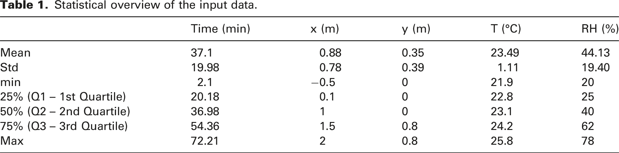
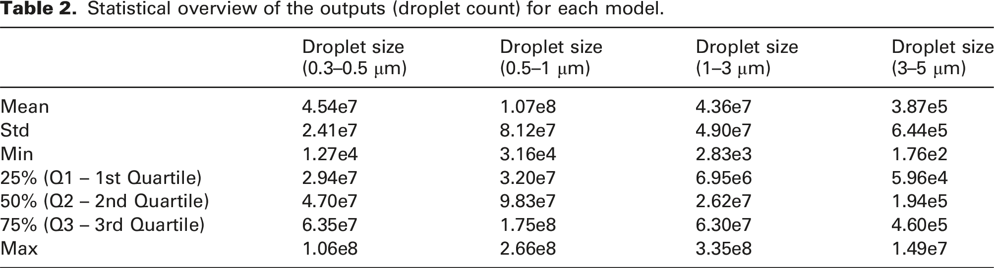
Statistical overview of the outputs (droplet count) for each model.

	Droplet size (0.3–0.5 μm)	Droplet size (0.5–1 μm)	Droplet size (1–3 μm)	Droplet size (3–5 μm)
Mean	4.54e7	1.07e8	4.36e7	3.87e5
Std	2.41e7	8.12e7	4.90e7	6.44e5
Min	1.27e4	3.16e4	2.83e3	1.76e2
25% (Q1 – 1st Quartile)	2.94e7	3.20e7	6.95e6	5.96e4
50% (Q2 – 2nd Quartile)	4.70e7	9.83e7	2.62e7	1.94e5
75% (Q3 – 3rd Quartile)	6.35e7	1.75e8	6.30e7	4.60e5
Max	1.06e8	2.66e8	3.35e8	1.49e7

In the supervised learning approach, for the development and assessment of ML models, the entire dataset was typically divided into two parts: the training set and the testing set. The training set, which typically comprises around 70%–90% of the entire dataset, was used to train the ML model by minimizing the error between predicted and actual data. The testing set contains unseen data (i.e. 10%–30% of the entire dataset, which was not used in the training phase) and was utilized to evaluate the performance of the model. In this study, 80% of the entire dataset was used to train the ML models, with the remaining 20% reserved for testing.

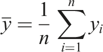
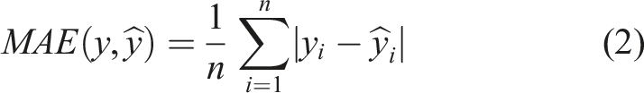
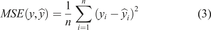
To develop and evaluate the ML models, several algorithms, including Decision Tree (DT), Random Forest (RF) and Artificial Neural Network (ANN), were tested.^50–54 The performance of the models was assessed using the R² score, mean absolute error (MAE), mean squared error (MSE) and maximum error for both training and testing. These parameters are defined by equations (1)–(4), as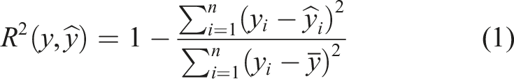

R^{2} (y, \hat{y}) = 1 - \frac{\sum_{i = 1}^{n} {(y_{i} - {\hat{y}}_{i})}^{2}}{\sum_{i = 1}^{n} {(y_{i} - \bar{y})}^{2}}

(1)

\bar{y} = \frac{1}{n} \sum_{i = 1}^{n} y_{i}

M A E (y, \hat{y}) = \frac{1}{n} \sum_{i = 1}^{n} | y_{i} - {\hat{y}}_{i} |

(2)

M S E (y, \hat{y}) = \frac{1}{n} \sum_{i = 1}^{n} {(y_{i} - {\hat{y}}_{i})}^{2}

(3)

Max e r r o r (y, \hat{y}) = \max (| y_{i} - {\hat{y}}_{i} |)

(4)

where

{\hat{y}}_{i}

represents the predicted values of the i^th sample,

y_{i}

is the corresponding actual value and

n

is the number of samples. The hyperparameters in these models were tuned using the grid search technique, and the models were built and tested using Python’s scikit-learn library.⁵⁵ After removing a few instances with missing values (data cleaning), different feature scaling methods like standardization, normalization, power and log transformation and robust scaler were tested to ensure that each feature was more or less normally distributed (i.e. has a bell-shaped histogram) and all features were of the same order of magnitude. In general, feature scaling can improve the model’s performance significantly (e.g. see our previous studies.^56,57).

Overfitting is one of the key reasons why ML algorithms perform poorly.^58,59 This phenomenon happens when the ML model over-trains itself to the point that it fits the training data too closely, subsequently failing to make reliable predictions for testing data. In the current investigation, various methods were employed to prevent overfitting. For the DT model, the maximum depth of the tree and the minimum number of samples required at a leaf node were examined. For the RF model, the number of trees in the forest, the maximum depth of the tree, as well as the minimum number of samples needed at a leaf node were analysed. For the ANN approach, L2 regularization technique was applied. In the ANN approach, various numbers for hidden layers, neurons, learning rates, alpha (the parameter related to L2 regularization) and epochs (iterations) were analysed in the grid search. Moreover, different activation functions, including the identity, the logistic sigmoid, the hyperbolic tangent and the rectified linear unit (relu), and two solvers for optimization (stochastic gradient descent (sgd) and ADAM (this name was derived from adaptive moment estimation)⁶⁰ were tested. Clearly, many terms, parameters and models related to ML algorithms have been mentioned so far. Explaining the details of these parameters and models is beyond the current scope of the article, so interested readers are referred to several books and papers.^{50–55,58,60–62}

Developing an empirical correlation along the x axis

To estimate the number of droplets (N) as a function of space and time, with a diameter of 0.3–0.5 μm for a prolonged period (e.g. 1 h), an empirical correlation was developed. Very fine droplets were considered since they could easily spread through the room and remain in the air for several hours. To develop this correlation, the experimental data along the cough direction (y = 0 and x > 0; locations 1–5 shown in Figure 2) was used. Additionally, experiments were performed at an ambient temperature of 23 ± 1°C but different RHs (20%–78%) were selected. In this case, since the temperature variation is not significant, it can be assumed that N is a function of distance (x), time (t) and RH. The main reason for this simplification (ignoring the effects of air temperature) is that in most indoor environments, RH changes in a wide range, but the change in ambient temperature is not considerable (typically between 22 and 24°C). Using the entire dataset (locations 1–11 in Figure 2) makes the regression problem more challenging, requiring more advanced methods like ML. The development of ML models based on the entire experimental data was discussed in the previous section.

As shown in Figure 2, the signal of the droplet count is extremely irregular. Although it might not be a big challenge to train the ML models (all these fluctuations were included in the training of the ML models), these fluctuations adversely affect the accuracy of the empirical correlation. To develop an empirical correlation, the initial step is to eliminate these fluctuations using appropriate filters and identify the key trends. In the current study, similar to our previous work,⁶³ the Savitzky–Golay (SG) filter in MATLAB was employed to smooth out those signals.⁶⁴ The SG filter was typically applied to a noisy signal whose frequency span is large. In this method, the least-squares error in fitting a polynomial to frames of noisy data was minimized to perform the filtering.⁶⁴ In the present work, the SG filter of polynomial order 3–6 was utilized for data frames of length 61–71. Figure 3 shows the signals of droplet count after applying the SG filter. As can be seen, this filter is effective in extracting the main trend from such a noisy time-series data, which is an essential step in developing the empirical correlation.

Figure 3.

An example for using an SG filter to extract the main trend from the experimental data.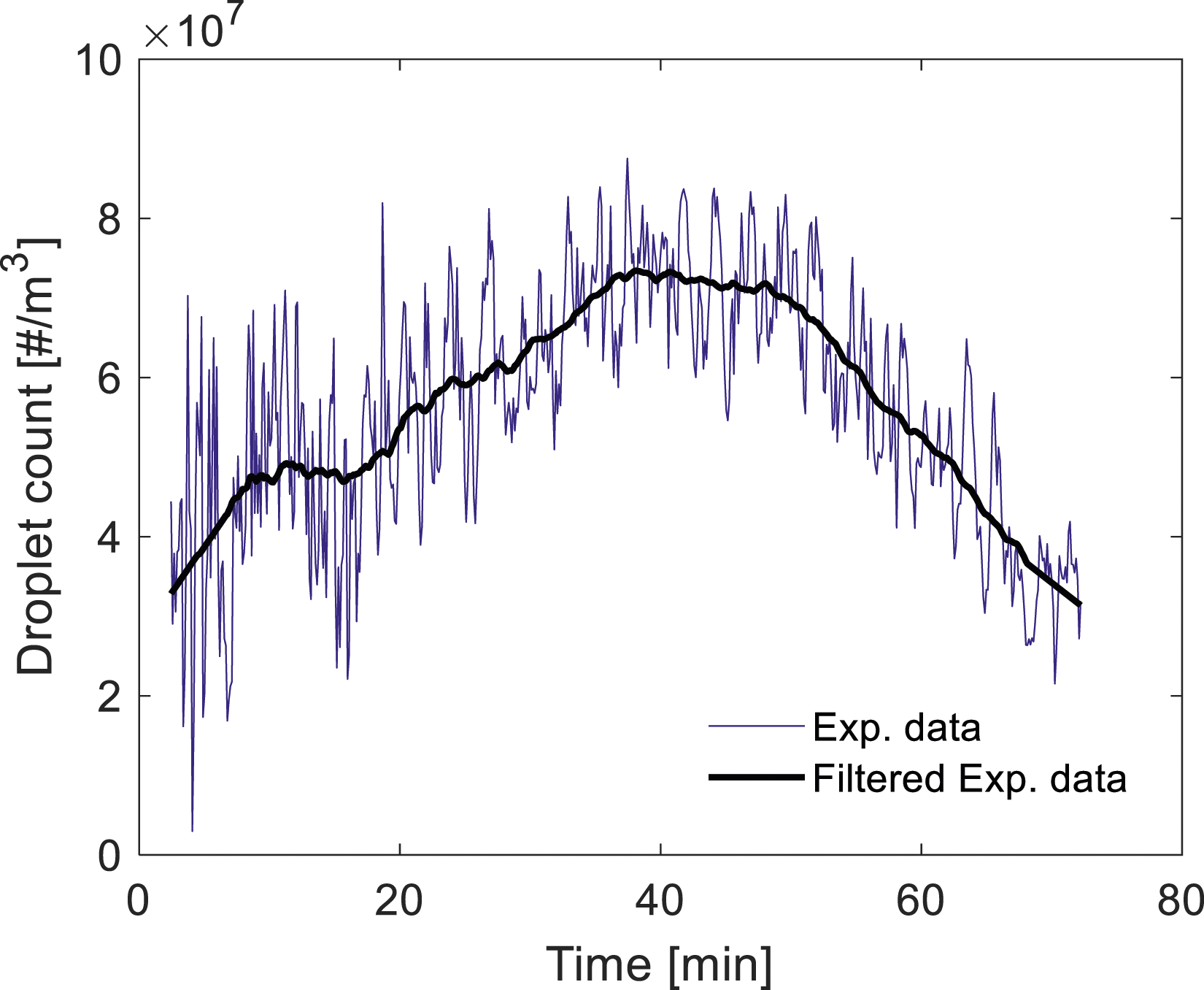

Results

The ML models

As previously outlined, three different ML approaches (i.e. DT, RF and ANN) along with various feature scaling and overfitting prevention techniques were tested to develop four accurate ML models for four size bins (0.3–0.5 μm, 0.5–1 μm, 1–3 μm and 3–5 μm). After analysing all the MAE, MSE, maximum error and R² values obtained from different ML algorithms for both training and testing phases, the performance of RF models was found to be slightly better than that of ANN and DT models. The values of R², MSE and maximum error obtained from testing (20% of the entire dataset) these models are reported in Tables 3–5. As can be seen, the values of R² for RF models are greater than 0.9, indicating that the models can accurately predict the outputs. For the ANN and DT models, the R² values are marginally lower. The RF models also exhibit slightly lower MSE and maximum error values compared to ANN and DT models, indicating superior accuracy and precision in the evaluated dataset. Furthermore, in alignment with previous studies,^65–67 our analysis revealed that ANN models demonstrated higher computational requirements compared to DT and RF models. Therefore, the RF models are only discussed hereafter. For the selected RF models, the MinMaxScaler (which is a common data normalization technique) was used to rescale variables into the range [0,1] and the number of trees in the forest was 30. Moreover, for these models, the maximum depth of the tree and the minimum number of samples needed at a leaf node were 15 and 2, respectively.

Table 3.

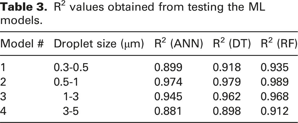
R² values obtained from testing the ML models.

Model #	Droplet size (μm)	R² (ANN)	R² (DT)	R² (RF)
1	0.3-0.5	0.899	0.918	0.935
2	0.5-1	0.974	0.979	0.989
3	1-3	0.945	0.962	0.968
4	3-5	0.881	0.898	0.912

Table 4.

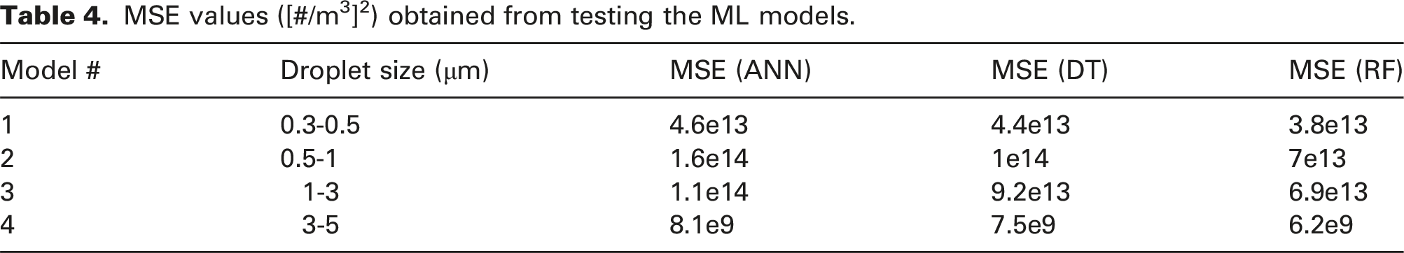
MSE values ([#/m³]²) obtained from testing the ML models.

Model #	Droplet size (μm)	MSE (ANN)	MSE (DT)	MSE (RF)
1	0.3-0.5	4.6e13	4.4e13	3.8e13
2	0.5-1	1.6e14	1e14	7e13
3	1-3	1.1e14	9.2e13	6.9e13
4	3-5	8.1e9	7.5e9	6.2e9

Table 5.

Maximum error ([#/m³]) values obtained from testing the ML models.

Model #	Droplet size (μm)	Max error (ANN)	Max error (DT)	Max error (RF)
1	0.3-0.5	5.3e7	5.2e7	4.2e7
2	0.5-1	2e8	1.8e8	7e7
3	1-3	1.53e8	1.42e8	1.1e8
4	3-5	4e6	3.7e6	2.9e6

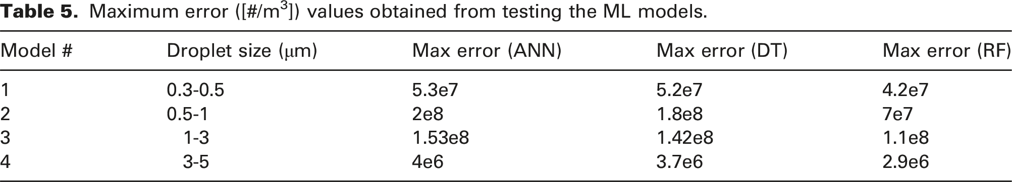
Figure 4 demonstrates the ability of the four RF models to predict the droplet count and size distributions at varying locations, times, relative humidities and air temperatures with high accuracy. The figure displays the outcomes of the tests carried out on the chosen RF models, using 20% of the entire dataset. The horizontal axis represents the actual data from the experiments, while the vertical axis shows the predicted values from the RF models. The data in this study (as depicted in Figure 2) exhibit pronounced irregularities, fluctuations and remarkable spikes. This nature presents challenges for regression analysis.^68,69 However, despite these complexities, Table 3 and Figure 4 demonstrate achieving an R² score greater than 0.9 which attests to the high accuracy of the RF models in performance and predictions.

Figure 4.

The predicted values resulting from the RF models versus the experimental data where 20% of the entire dataframe was used as a test set.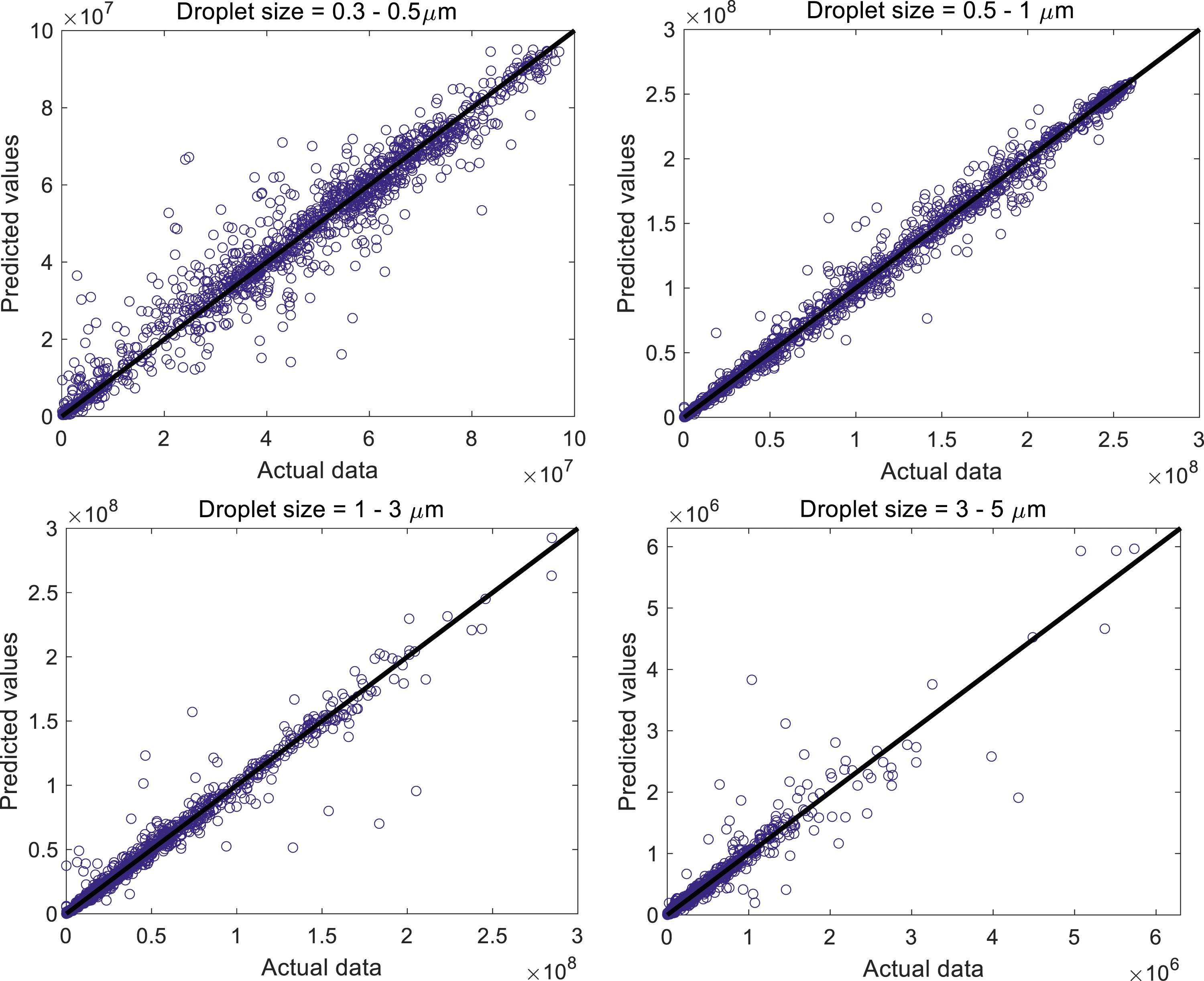

The R² score and accuracy achieved in the current study are comparable to those reported in similar works within the existing literature. For example, Liu et al.⁴⁴ developed various machine learning models to forecast healthcare workers' exposure to exhaled aerosols in an operating room, with a particular focus on breathing patterns. Cough typically results in higher turbulent intensity compared to breathing; therefore, the data presented in the current study were expected to be more chaotic and irregular. Evaluating four algorithms: random forest, adaptive boosting, gradient boosting decision tree (GBDT) and extreme gradient boosting (XGboost), Liu et al.⁴⁴ found that the random forest model exhibited the best overall performance, aligning with our observations in the current study. Their random forest models achieved R² scores ranging from around 0.78 to 0.98. In contrast, our random forest models demonstrated higher accuracy, with R² scores ranging between 0.912 and 0.989, underscoring the robustness of our models. In another study, Hariharan⁴⁵ explored the impact of daily mean temperature, absolute humidity and average wind speed on the attack and mortality rates of COVID-19 in Delhi, India, using a random forest algorithm. The R² scores for that random forest model were 0.92 for the attack rate and 0.88 for the mortality rate, which are lower compared to the values obtained in the current study.

An additional test was also conducted to evaluate the performance and accuracy of the four RF models for a prolonged period of time. To carry out this test, the experimental data obtained from the measurements at a specific location, RH and air temperature were employed. Clearly, since the location, RH and air temperature were fixed, the droplet count and size distributions depended only on time. Here, the experimental data obtained from location 3, which was 1 m away from the manikin mouth (x = 1 m and y = 0), at RH = 67% and air temperature of 24.2°C were considered. These data were not included in the training and testing phases mentioned above and were only used to verify the predictions of the four RF models for a prolonged period. Figure 5 presents a comparison of the RF models’ predictions with these experimental data. As can be seen, there is a good agreement between the predicted values and the experimental data, revealing that the models can accurately predict the trends and the distributions.

Figure 5.

The predicted values obtained from the RF models (red dots) versus the experimental data (blue dots) where x = 1 m, y = 0 (i.e. location 3), RH = 67% and air temperature was 24.2°C.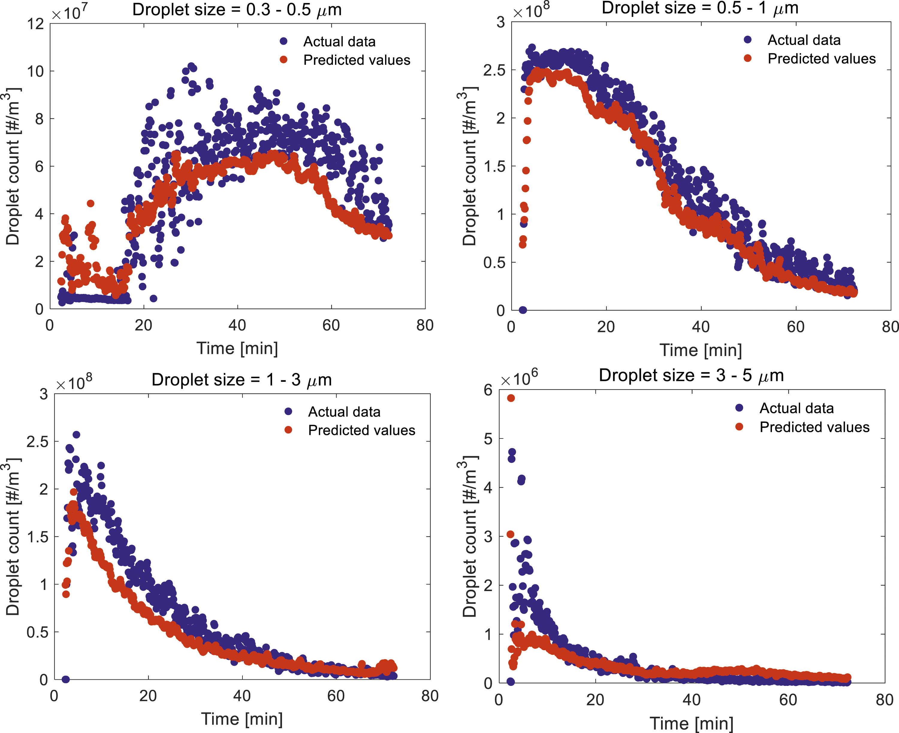

The empirical correlation

With the aid of the SG filter, we can have more practical discussions regarding the variations in droplet size and count distributions as different parameters are varied. For instance, in Figure 6, the effect of axial distance from the manikin mouth (x) on droplet count at different RH values is shown after filtering. The droplet size range in this figure was between 0.3 and 0.5 μm. As demonstrated, if we kept the RH constant and increased the axial distance x, the distribution of droplet counts shifted towards the left and its peak value was increased.

Figure 6.

Effect of axial distance (x) on droplet count distribution at various RH values.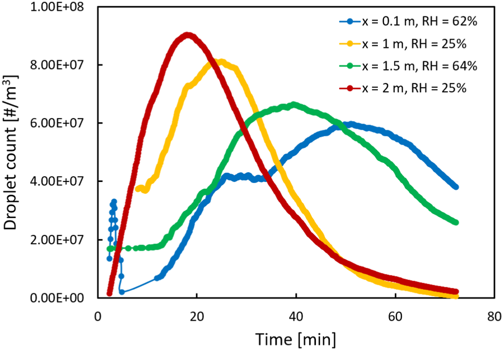

In general, it is demonstrated that the number of droplets tends to increase initially with time, but then decreases. The following two functions, equations (5) and (6), which were derived from the general forms of the probability density function (PDF) for log-normal and normal distributions, can be used to describe this trend: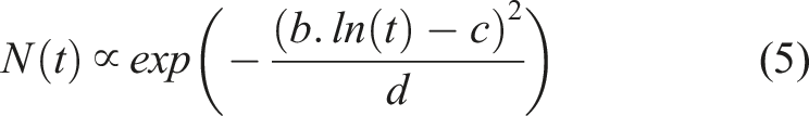

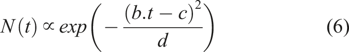
N (t) \propto \exp (- \frac{{(b . \ln (t) - c)}^{2}}{d})

(5)

N (t) \propto \exp (- \frac{{(b . t - c)}^{2}}{d})

(6)

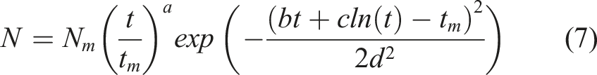
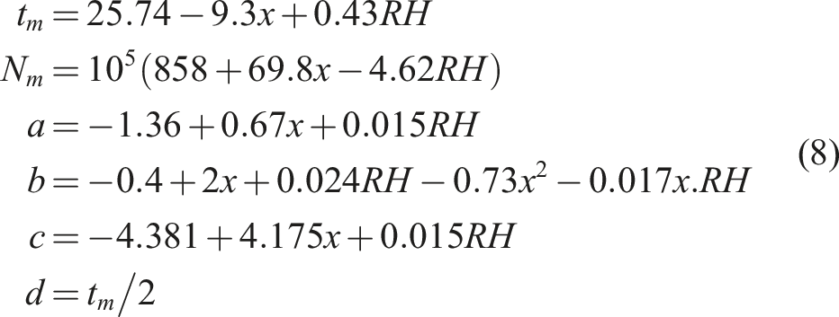
By increasing RH or decreasing x, the dependency of droplet counts on time shifts from the function given in equation (5) to the function in equation (6). As a result, both $t$ and $\ln (t)$ should be present inside the exponential function, and $b$ , $c$ and $d$ should be a function of RH and x. Eventually, the empirical correlations of equations (7) and (8) for droplet count (N) were obtained based on the assumptions mentioned in the previous section (e.g. the droplet size range is between 0.3 and 0.5 μm):

N = N_{m} {(\frac{t}{t_{m}})}^{a} \exp (- \frac{{(b t + c l n (t) - t_{m})}^{2}}{2 d^{2}})

(7)

t_{m} = 25.74 - 9.3 x + 0.43 R H N_{m} = 10^{5} (858 + 69.8 x - 4.62 R H) a = - 1.36 + 0.67 x + 0.015 R H b = - 0.4 + 2 x + 0.024 R H - 0.73 x^{2} - 0.017 x . R H c = - 4.381 + 4.175 x + 0.015 R H d = t_{m} / 2

(8)

Here, RH is in %, x is in m, t and $t_{m}$ are in min, N and $N_{m}$ are $particle count / m^{3}$ and $# / m^{3}$ , respectively. The predictions of the proposed correlation were compared with the original experimental data as well as the filtered experimental data in Figure 7. As shown, the correlation was able to predict the droplet count for a long period of time and for a wide range of distances and RHs. The above correlation is useful for CFD validations and rough estimations of droplet count in indoor environments. For instance, it can aid in determining the potential risk of pathogen transmission in crowded public spaces, like hospitals and schools, under varying RH conditions. It also can help in managing and optimizing occupancy density within a room. Additionally, the correlation can support the design and optimization (e.g. the power and time of operation) of air purification systems by providing initial estimates of droplet count under different environmental conditions. Overall, these rough estimations offer valuable insights for evaluating and mitigating potential indoor airborne transmission of contaminants.

Figure 7.

Comparison between the predictions of the empirical correlation and the filtered/unfiltered experimental data.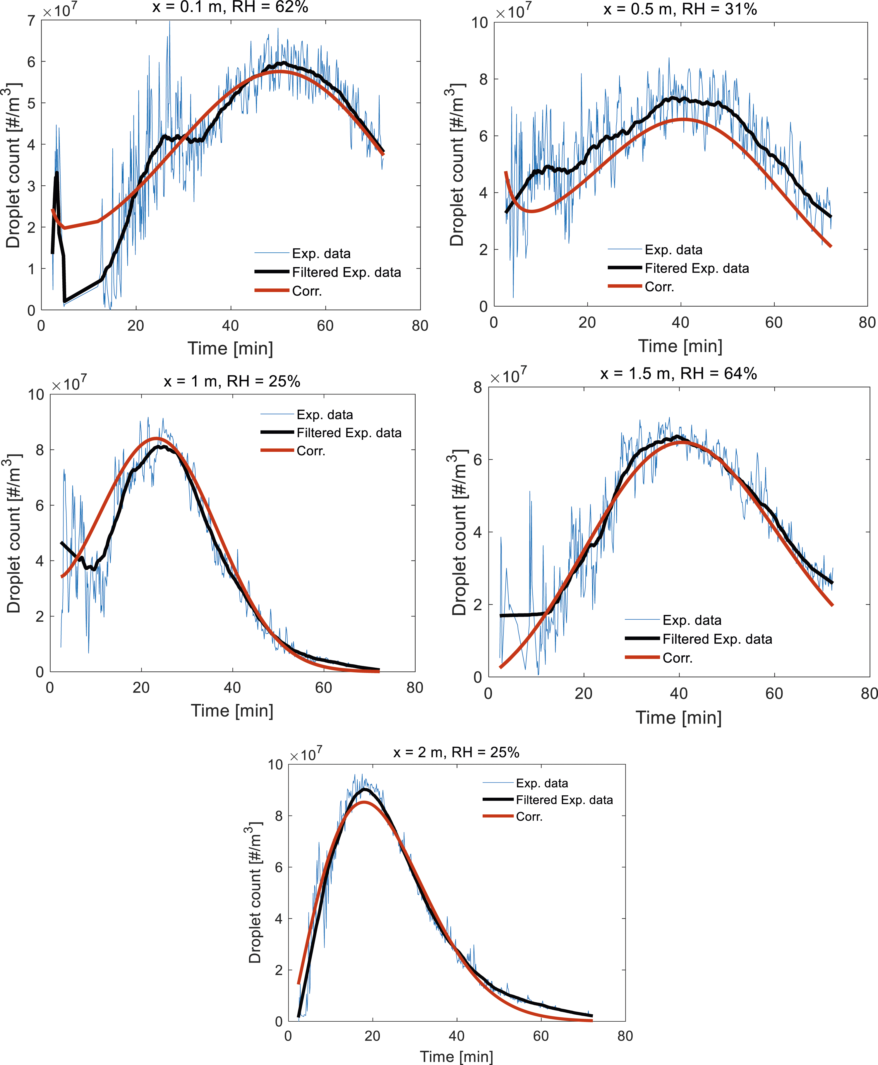

Summary and conclusions

In summary, this study has developed both a Machine Learning (ML) model and an empirical correlation to predict the temporal and spatial distributions of droplet count and size following a cough in an indoor environment over an extended period, at varying relative humidity levels and air temperatures. The dataframe was built using the experimental data obtained under real conditions. Three different ML algorithms, namely, Decision Tree, Random Forest and Artificial Neural Network, were tested, and it was found that the Random Forest model performed slightly better than the other approaches. The correlation and the ML model developed in the present study are useful to estimate the cough-emitted droplet in-flight behaviour in an indoor environment, which can aid in developing effective strategies to control and reduce the spread of infectious pathogens. In addition, these models can be used to validate numerical and Computational Fluid Dynamics (CFD) simulations.

Footnotes

Acknowledgements

The authors thank Mr Kai Lordly for his assistance with this research.

Authors contributions

Mehdi Jadidi: Conceptualization, Methodology, Validation, Analysis, Writing – original draft. Ahmet E. Karataş: Data collection, Material preparation, Writing – Review & Editing. Seth B. Dworkin: Supervision, Writing – Review & Editing, Funding acquisition. All authors read and approved the final manuscript.

Declaration of conflicting interests

The author(s) declared no potential conflicts of interest with respect to the research, authorship, and/or publication of this article.

Funding

The author(s) received no financial support for the research, authorship, and/or publication of this article.

ORCID iD

Mehdi Jadidi

References

Lordly

Kober

Jadidi

Antoun

Dworkin

Karataş

. Understanding lifetime and dispersion of cough-emitted droplets in air. Indoor Built Environ 2023; 32(10): 1929–1948. DOI: 10.1177/1420326X221098753.

Wang

Prather

Sznitman

Jimenez

Lakdawala

Tufekci

Marr

. Airborne transmission of respiratory viruses. Science 2021; 373: 6558. DOI: 10.1126/science.abd9149.

Jayaweera

Perera

Gunawardana

Manatunge

. Transmission of COVID-19 virus by droplets and aerosols: a critical review on the unresolved dichotomy. Environ Res 2020; 188: 109819.

McNeill

. Airborne transmission of SARS-CoV-2: evidence and implications for engineering controls. Annu Rev Chem Biomol Eng 2022; 13: 123–140. DOI: 10.1146/annurev-chembioeng-092220-111631.

Henriques

Mounet

Aleixo

Elson

Devine

Azzopardi

Andreini

Rognlien

Tarocco

Tang

. Modelling airborne transmission of SARS-CoV-2 using CARA: risk assessment for enclosed spaces. Interface Focus 2022; 12: 20210076.

Buonanno

Robotto

Brizio

Morawska

Civra

Corino

Lembo

Ficco

Stabile

. Link between SARS-CoV-2 emissions and airborne concentrations: closing the gap in understanding. J Hazard Mater 2022; 428: 128279.

Caldas

Carneiro

Higa

Monteiro

da Silva

da Costa

Durigon

Tanuri

de Souza

. Ultrastructural analysis of SARS-CoV-2 interactions with the host cell via high resolution scanning electron microscopy. Sci Rep 2020; 10: 16099.

Dabisch

Schuit

Herzog

Beck

Wood

Krause

Miller

Weaver

Freeburger

Hooper

Green

Williams

Holland

Bohannon

Wahl

Yolitz

Hevey

Ratnesar-Shumate

. The influence of temperature, humidity, and simulated sunlight on the infectivity of SARS-CoV-2 in aerosols. Aerosol Sci Technol 2021; 55: 142–153.

Fears

Klimstra

Duprex

Hartman

Weaver

Plante

Mirchandani

Plante

Aguilar

Fernández

Nalca

Totura

Dyer

Kearney

Lackemeyer

Bohannon

Johnson

Garry

Reed

Chad

. Persistence of severe acute respiratory syndrome Coronavirus 2 in aerosol suspensions. Emerg Infect Dis 2020; 26: 2168–2171.

10.

van Doremalen

Bushmaker

Morris

Holbrook

Gamble

Williamson

Tamin

Harcourt

Thornburg

Gerber

Lloyd-Smith

de Wit

Munster

. Aerosol and surface stability of SARS-CoV-2 as compared with SARS-CoV-1. N Engl J Med 2020; 382: 1564–1567.

11.

Schuit

Ratnesar-Shumate

Yolitz

Williams

Weaver

Green

Miller

Krause

Beck

Wood

Holland

Bohannon

Freeburger

Hooper

Biryukov

Altamura

Wahl

Hevey

Dabisch

. Airborne SARS-CoV-2 is rapidly inactivated by simulated sunlight. J Infect Dis 2020; 222: 564–571.

12.

Ratnesar-Shumate

Williams

Green

Krause

Holland

Wood

Bohannon

Boydston

Freeburger

Hooper

Beck

Yeager

Altamura

Biryukov

Yolitz

Schuit

Wahl

Hevey

Dabisch

. Simulated sunlight rapidly inactivates SARS-CoV-2 on surfaces. J Infect Dis 2020; 222: 214–222.

13.

Smither

Eastaugh

Findlay

Lever

. Experimental aerosol survival of SARS-CoV-2 in artificial saliva and tissue culture media at medium and high humidity. Emerg Microb Infect 2020; 9: 1415–1417.

14.

Gupta

Lin

Chen

. Flow dynamics and characterization of a cough. Indoor Air 2009; 19: 517–525.

15.

Yang

Lee

GWM

Chen

C-M

C-C

K-P

. The size and Concentration of droplets generated by Coughing in human subjects. J Aerosol Med 2007; 20: 484–494.

16.

Welsch

. The impact of mask usage on COVID-19 deaths: evidence from US counties using a quasi-experimental approach. B E J Econom Anal Policy 2022; 22: 1–28. DOI: 10.1515/bejeap-2021-0157.

17.

Koroteeva

Shagiyanova

. Infrared-based visualization of exhalation flows while wearing protective face masks. Phys Fluids 2022; 34: 011705. DOI: 10.1063/5.0076230.

18.

World Health Organization . Roadmap to improve and ensure good indoor ventilation in the context of COVID-19. Geneva: WHO, 2021.

19.

Fontes

Reyes

Ahmed

Kinzel

. A study of fluid dynamics and human physiology factors driving droplet dispersion from a human sneeze. Phys Fluids 2020; 32: 111904. DOI: 10.1063/5.0032006.

20.

Olivieri

Cavaiola

Mazzino

Rosti

. Transport and evaporation of virus-containing droplets exhaled by men and women in typical cough events. Meccanica 2022; 57: 567–575.

21.

Bourouiba

. Turbulent gas clouds and respiratory pathogen emissions: potential implications for reducing transmission of COVID-19. JAMA 2020; 323: 1837–1838. DOI: 10.1001/jama.2020.4756.

22.

Sajadi

Habibzadeh

Vintzileos

Shokouhi

Miralles-Wilhelm

Amoroso

. Temperature, humidity, and latitude analysis to estimate potential spread and seasonality of Coronavirus disease 2019 (COVID-19). JAMA Netw Open 2020; 3: e2011834. DOI: 10.1001/jamanetworkopen.2020.11834.

23.

Jarvis

. Aerosol transmission of SARS-CoV-2: physical principles and implications. Front Public Health 2020; 8: 590041. DOI: 10.3389/fpubh.2020.590041.

24.

Zhao

Luzzatto-Fegiz

Cui

Zhu

. COVID-19: effects of environmental Conditions on the propagation of respiratory droplets. Nano Lett 2020; 20: 7744–7750.

25.

Chong

Hori

Yang

Verzicco

Lohse

. Extended lifetime of respiratory droplets in a turbulent vapor puff and its implications on airborne disease transmission. Phys Rev Lett 2021; 126: 034502.

26.

Chaudhuri

Basu

Saha

. Analyzing the dominant SARS-CoV-2 transmission routes toward an ab initio disease spread model. Phys Fluids 2020; 32: 123306. DOI: 10.1063/5.0034032.

27.

Wang

Zhang

Zhu

Liu

Wang

. The motion of respiratory droplets produced by coughing. Phys Fluids 2020; 32: 125102. DOI: 10.1063/5.0033849.

28.

Wang

Wan

. Transport and fate of human expiratory droplets - a modeling approach. Phys Fluids 2020; 32: 083307. DOI: 10.1063/5.0021280.

29.

Noti

Blachere

McMillen

Lindsley

Kashon

Slaughter

Beezhold

. High humidity leads to loss of infectious influenza virus from simulated Coughs. PLoS One 2013; 8: e57485. DOI: 10.1371/journal.pone.0057485.

30.

Yang

Marr

. Dynamics of Airborne influenza A viruses indoors and dependence on humidity. PLoS One 2011; 6: e21481. DOI: 10.1371/journal.pone.0021481.

31.

Mirzaei

Moshfeghi

Motamedi

Sheikhnejad

Bordbar

. A simplified tempo-spatial model to predict airborne pathogen release risk in enclosed spaces: an Eulerian-Lagrangian CFD approach. Build Environ 2022; 207: 108428. DOI: 10.1016/j.buildenv.2021.108428.

32.

Mesgarpour

Abad

JMN

Alizadeh

Wongwises

Doranehgard

Jowkar

Karimi

. Predicting the effects of environmental parameters on the spatio-temporal distribution of the droplets carrying coronavirus in public transport – a machine learning approach. Chem Eng J 2022; 430: 132761. DOI: 10.1016/j.cej.2021.132761.

33.

Mesgarpour

Abad

JMN

Alizadeh

Wongwises

Doranehgard

Ghaderi

Karimi

. Prediction of the spread of Corona-virus carrying droplets in a bus - a computational based artificial intelligence approach. J Hazard Mater 2021; 413: 125358. DOI: 10.1016/j.jhazmat.2021.125358.

34.

Motamedi Zoka

Moshfeghi

Bordbar

Mirzaei

Sheikhnejad

. A CFD approach for risk assessment based on airborne pathogen transmission. Atmosphere 2021; 12: 986. DOI: 10.3390/atmos12080986.

35.

Bahiuddin

Wibowo

Syairaji

Putra

Pandito

Maulana

Prastica

RMS

Nazmi

. A systematic approach to predict the behavior of cough droplets using feedforward neural networks method. Fluid 2021; 6: 76. DOI: 10.3390/fluids6020076.

36.

Božič

Kanduč

. Relative humidity in droplet and airborne transmission of disease. J Biol Phys 2021; 47: 1–29. DOI: 10.1007/s10867-020-09562-5.

37.

Trivedi

Gkantonas

Mesquita

LCC

Iavarone

de Oliveira

Mastorakos

. Estimates of the stochasticity of droplet dispersion by a cough. Phys Fluids 2021; 33: 115130. DOI: 10.1063/5.0070528.

38.

Kassania

Kassanib

Wesolowskic

Schneidera

Detersa

. Automatic detection of Coronavirus disease (COVID-19) in X-ray and CT images: a machine learning based approach. Biocybern Biomed Eng 2021; 41(3): 867–879. DOI: 10.1016/j.bbe.2021.05.013.

39.

Despotovic

Ismael

Cornil

McCall

Fagherazzi

. Detection of COVID-19 from voice, cough and breathing patterns: dataset and preliminary results. Comput Biol Med 2021; 138: 104944. DOI: 10.1016/j.compbiomed.2021.104944.

40.

Imran

Posokhova

Qureshi

Masood

Riaz

Ali

John

Hussain

MDI

Nabeel

. AI4COVID-19: AI enabled preliminary diagnosis for COVID-19 from cough samples via an app. Inform Med Unlocked 2020; 20: 100378. DOI: 10.1016/j.imu.2020.100378.

41.

Yan

Sun

Fang

. Semi-surrogate modelling of droplets evaporation process via XGBoost integrated CFD simulations. Sci Total Environ 2023; 895: 164968. DOI: 10.1016/j.scitotenv.2023.164968.

42.

Elsarraj

Mahmoudi

Keshmiri

. Quantifying indoor infection risk based on a metric-driven approach and machine learning. Build Environ 2024; 251: 111225.

43.

Han

Peng

Chen

. Spatiotemporal distribution prediction of coughing airflow at mouth based on machine learning - Part I: study on boundary conditions at mouth in numerical simulation of cough airflow. E3S Web of Conferences 2023; 396: 01015. DOI: 10.1051/e3sconf/202339601015.

44.

Liu

Huang

Chu

Lin

Jiang

Yao

Fan

. A novel approach for predicting the concentration of exhaled aerosols exposure among healthcare workers in the operating room. Build Environ 2023; 245: 110867. DOI: 10.1016/j.buildenv.2023.110867.

45.

Hariharan

. Random forest regression analysis on combined role of meteorological indicators in disease dissemination in an Indian city: a case study of New Delhi. Urban Clim 2021; 36: 100780. DOI: 10.1016/j.uclim.2021.100780.

46.

Gralton

Tovey

McLaws

Rawlinson

. The role of particle size in aerosolised pathogen transmission: a review. J Infect 2011; 62: 1–13.

47.

Liu

Novoselac

. Transport of airborne particles from an unobstructed cough jet. Aerosol Sci Technol 2014; 48: 1183–1194.

48.

Lee

Yoo

Ryu

Ham

Lee

Yeo

Min

Yoon

. Quantity, size distribution, and characteristics of cough-generated aerosol produced by patients with an upper respiratory tract infection. Aerosol Air Qual Res 2019; 19: 840–853. DOI: 10.4209/aaqr.2018.01.0031.

49.

Jiang

Gradus

Rosellini

. Supervised machine learning: a brief primer. Behav Ther 2020; 51: 675–687. DOI: 10.1016/j.beth.2020.05.002.

50.

Breiman

. Random forests. Mach Learn 2001; 45: 5–32. DOI: 10.1023/A:1010933404324.

51.

Schmidhuber

. Deep Learning in neural networks: an overview. Neural Network 2015; 61: 85–117. DOI: 10.1016/j.neunet.2014.09.003.

52.

Song

. Decision tree methods: applications for classification and prediction. Shanghai Arch Psychiatry 2015; 27: 130–135. DOI: 10.11919/j.issn.1002-0829.215044.

53.

Basheer

Hajmeer

. Artificial neural networks: fundamentals, computing, design, and application. J Microbiol Methods 2000; 43: 3–31. DOI: 10.1016/S0167-7012(00)00201-3.

54.

Jain

Mao

Mohiuddin

. Artificial neural networks: a tutorial. Computer 1996; 29: 31–44. DOI: 10.1109/2.485891.

55.

Pedregosa

Varoquaux

Gramfort

Michel

Thirion

Grisel

Blondel

Prettenhofer

Weiss

Dubourg

Vanderplas

Passos

Cournapeau

Brucher

Perrot

Duchesnay

. Scikit-learn: machine learning in Python. J Mach Learn Res 2011; 12: 2825–2830.

56.

Jadidi

Kostic

Zimmer

Dworkin

. An artificial neural network for the low-cost prediction of soot emissions. Energies 2020; 13: 4787. DOI: 10.3390/en13184787.

57.

Khanehzar

Jadidi

Zimmer

Dworkin

. Application of machine learning for the low-cost prediction of soot concentration in a turbulent flame. Environ Sci Pollut Res 2023; 30: 27103–27112. DOI: 10.1007/s11356-022-24161-8.

58.

. The random subspace method for constructing decision forests. IEEE Trans Pattern Anal Mach Intell 1998; 20: 832–844. DOI: 10.1109/34.709601.

59.

Srivastava

Hinton

Krizhevsky

Sutskever

Salakhutdinov

. Dropout: a simple way to prevent neural networks from overfitting. J Mach Learn Res 2014; 15: 1929–1958.

60.

Kingma

. Adam: A method for stochastic optimization. In: 3rd International Conference on Learning Representations - ICLR 2015, San Diego, USA, 7–9 May 2015. DOI: 10.48550/arXiv.1412.6980.

61.

Svetnik

Liaw

Tong

Culberson

Sheridan

Feuston

. Random forest: a Classification and regression tool for compound Classification and QSAR modeling. J Chem Inf Comput Sci 2003; 43: 1947–1958. DOI: 10.1021/ci034160g.

62.

Quinlan

. Induction of decision trees. Mach Learn 1986; 1: 81–106. DOI: 10.1023/A:1022643204877.

63.

Garmeh

Jadidi

Lamarre

Dolatabadi

. Cold spray gas flow dynamics for on and off-axis nozzle/substrate hole geometries. J Therm Spray Technol 2023; 32: 208–225. DOI: 10.1007/s11666-022-01487-w.

64.

Schafer

. What is a savitzky-golay filter? IEEE Signal Process Mag 2011; 28: 111–117. DOI: 10.1109/MSP.2011.941097.

65.

Roßbach

Neural networks vs. Random forests – does it always have to be deep learning? Ger Frankf Sch Financ Manag. https://blog.frankfurt-school.de/neural-networks-vs-random-forests-does-it-always-have-to-be-deep-learning/ (2018, accessed 14 March 2024).

66.

Song

. Random forest approach in modeling the flow stress of 304 stainless steel during deformation at 700°C–900°C. Materials 2021; 14: 1812. DOI: 10.3390/ma14071812.

67.

Mousemi

Jadidi

Dworkin

Bushe

. Application of machine learning in low-order manifold representation of chemistry in turbulent flames. Combust Theor Model 2023; 27: 83–102. DOI: 10.1080/13647830.2022.2153740.

68.

Branco

Torgo

Ribeiro

. SMOGN: a pre-processing approach for imbalanced regression. Proceedings of Machine Learning Research 2017; 74: 36–50, First International Workshop on Learning with Imbalanced Domains: Theory and Applications, Skopje, Macedonia, 22 September 2017.

69.

Yang

Zha

Chen

Wang

Katabi

. Delving into deep imbalanced regression. Proceedings of the 38th International Conference on Machine Learning, Virtual (online) 2021; 139: 11842–11851.

Estimating droplet size and count distributions over a prolonged period of time following a cough in indoor environments

Abstract

Keywords

Introduction

Methodology

Collecting data from experiments

Experimental setup

Experimental measurements and data structure

Complexity in interpretation of experimental results and necessity of developing machine learning models

Developing machine learning models

Developing an empirical correlation along the x axis

Results

The ML models

The empirical correlation

Summary and conclusions

Footnotes

Acknowledgements

Authors contributions

Declaration of conflicting interests

Funding

ORCID iD

References