Fluorescence spectroscopy and machine learning methods for detection of Alzheimer's disease from circulating white blood cells

Abstract

Background

Alzheimer's disease (AD) is the most common cause of dementia whose prevalence is projected to increase significantly in the coming decades. The recent advent of disease modifying therapies is a welcome development; however, it is also now apparent that early treatment maximizes the benefits of these drugs. Therefore, it is important to develop reliable methods of disease detection, preferably from an easily accessible matrix such as blood.

Objective

To develop a method for detecting AD from circulating white blood cells using spectral confocal microscopy.

Methods

Using K114-stained wild type and 5xFAD transgenic mouse cortical sections as proof-of-principle, spectral imaging of K114 fluorescence coupled with a signal processing/machine learning pipeline (spectral wavelet decomposition, dimensionality reduction, support vector machine classifier) can reliably distinguish non-plaque background parenchyma in the two strains. We then performed immunoprecipitation of Aβ from peripheral blood mononuclear cells (PBMCs) obtained from non-neurological controls and histopathologically-proven AD cases. We spectrally imaged the immunobeads labeled with K114, then used similar machine learning methods to classify control versus AD samples.

Results

Normal-appearing non-plaque 5xFAD background was reliably distinguished from wild type mouse brain. We could also classify AD with a high degree of reliability (area under the receiver operating curve = 0.95, p = 6.1e-5) and predict neuropathological scores from these blood elements (R = 0.89).

Conclusions

Our spectral imaging method, together with automated machine learning analysis of spectral micrographs, using readily obtainable PBMCs from blood, represents a potentially useful approach for detection of AD in living subjects.

Introduction

It is now generally accepted that most neurodegenerative disorders, including Alzheimer's disease (AD), are based in large part on misfolding of one or more brain proteins.^1,2 Whether this is a primary driver of pathogenesis, or a consequence of a more fundamental underlying disease process, is still debated; moreover the initial trigger of the progressive proteopathy is not understood.^3–5 Nevertheless, neuropathological examination unequivocally shows deposition of protein aggregates, often coalescing into amyloids, in characteristic brain regions depending on the disease.^6,7 In the case of AD, amyloid-β (Aβ)-rich extracellular neuritic plaques and intra-neuronal neurofibrillary tangles represent the hallmark pathological characteristics of AD observed over a century ago using rudimentary silver stains. ⁸ Interestingly, such amyloid deposition appears to extend far beyond the well-known plaques and tangles, involving much of the otherwise normal appearing gray matter parenchyma.^9–11

Identifying larger pathological protein aggregates such as AD plaques and tangles is straightforward using conventional histological methods such as the Bielschowsky silver method or immunohistochemistry for Aβ or tau. Detecting more subtle amyloid accumulation is more challenging. β sheet-rich amyloids exhibit a unique property of high affinity binding to certain fluorescent probes such as Congo Red and thioflavins.^12–14 These undergo increases in fluorescence intensity when bound to amyloid fibrils, allowing visualization of such deposits in cells and tissues. Another interesting and very useful property of more recent amyloid dyes is their propensity to also change spectral shape when bound to β sheet-rich amyloids (for reviews, see^15–17). We and others have explored this property and its utility for detecting various amyloid morphotypes and more subtle amyloid accumulation in tissues.^16,18–21 Thus, careful selection of “spectrally active” probes, ones that undergo a measurable shift in spectral shape when bound to amyloid, coupled with spectral imaging, allows a much more sensitive and potentially specific detection of misfolded protein pathology. ²²

Peripheral blood mononuclear cells (PBMCs) have the ability to phagocytose pathogens and molecular debris.^23,24 Moreover, through interactions with cell adhesion molecules, the endothelium of the brain's microvasculature controls immune cell trafficking across the blood-brain barrier. ²⁵ We reasoned that migration of phagocytic leukocytes into the brain followed by their return into the circulation would allow these cells to carry a signature of diseased amyloid-laden brain parenchyma that might be detectable from peripheral blood using similar spectral fluorescence approaches. A proof-of-principle study on clinically- and cerebrospinal fluid (CSF)-confirmed healthy controls, subjects with mild cognitive impairment and those with established AD, showed that we were able to classify subjects with a high degree of accuracy. ²⁶ This study supported the hypothesis that spectral interrogation of circulating PBMCs may be a reliable method for detecting AD. In contrast to staining artificial fibrils or brain amyloid plaques with amyloid probes, which results in substantial spectral shifts, more subtle protein aggregates such as in the background brain parenchyma, or in phagocytic PBMCs, induce correspondingly subtle spectral changes whose shifts are not predictable. We leveraged the spectral variation of the amyloid-binding fluorescent probe K114,^27,28 a derivative of the classic amyloid dye Congo Red, together with spectral confocal microscopy to image transgenic AD mouse brain and circulating human PBMCs to detect AD signatures. We also developed machine learning methods to analyze subtle changes in spectral micrographs, in an automated and unbiased manner, with the goal of further increasing the sensitivity and reliability of these fluorescence detection methods. This paper describes approaches used on PBMCs obtained from human subjects (controls and those with AD) with matching neuropathology, as proof-of-principle illustrating how machine learning algorithms can be adapted to AD biomarker methods.

Methods

Reagents

NaHCO₃, Na₂CO₃ and glycerol were purchased from Sigma-Aldrich (St Louis, MO). K114 ((trans,trans)-1-bromo-2,5-bis(4-hydroxystyryl)benzene) was obtained from Tocris Bioscience (Bristol, UK), dissolved in dimethyl sulfoxide (DMSO) to yield a 100 mM stock solution and stored at −80°C. An aliquot was taken and diluted to 10 mM with DMSO immediately before use.

Preparation and imaging of 5xFAD mouse brain samples

Mouse tissue collection was conducted in accordance with the University of Calgary Animal Care Committee guidelines and approved under protocol #AC22-0149. Formalin-fixed, paraffin-embedded sections from 9-month-old wild-type (n = 5; 3 female, 2 male) and transgenic AD (5xFAD; n = 5; 2 female, 3 male) mice^29,30 were deparaffinized and rehydrated using xylene and decreasing ethanol gradient. Staining was carried out by incubating rehydrated slides in 10% ethanol: 90% 0.1 M sodium carbonate-bicarbonate buffer (pH 10) with 500 nM K114 in a glass coplin jar for 24 h on a shaker. The slides were then mounted in 50% phosphate-buffered saline (PBS)/glycerol after a quick rinse in PBS. Three 1k × 1k spectral images of the cortex per hemisphere were acquired (a total of 6 per mouse) on a A1R spectral confocal microscope equipped with a 1.1 NA 25× objective (Nikon, Japan) using 405 nm excitation and the spectral detector set to collect light within the 400-720 nm range.

Human subjects and PBMC sample collection

Use of human samples was approved by the University of Calgary Conjoint Health Research Ethics Board under protocol #REB22-1246. For proof-of-principle of machine learning methods, 12 frozen PBMC samples obtained from the National Centralized Repository for Alzheimer's Disease and Related Dementias (NCRAD) were selected based on clinically- and histologically-confirmed mild cognitive impairment/AD (Braak stage over 5; n = 6) and age-matched cognitively normal subjects based on the National Alzheimer's Coordinating Center (NACC) database (n = 6). Samples were stored at −80°C until use. Mean time between blood collection and death was approximately 1 year. Subject details are summarized in Supplemental Tables 1 and 2.

Aβ immunocapture by 4G8 antibody and K114 labeling

To adapt our fluorescent amyloid probe-based spectral analysis method ²⁶ to frozen PBMC samples, and to purify target amyloid proteins, we used immunoprecipitation with anti-Aβ antibody (4G8)-coated magnetic beads (Protein G SureBeadsTM, BioRad Laboratories). Briefly, 7.5 µg of 4G8 antibody was used per 150 µl of stock bead suspension. 4G8 was coupled with SureBeads for 15 min at RT under rotation. 12.5 µL of stock bead suspension was used for each PBMC sample. Approximately 50,000 frozen PBMCs from each sample were suspended in PBS and sonicated for 15 min before incubating with 4G8-coupled beads for 1 h at RT under rotation. Beads were washed with PBS-T and fixed in 1% formalin/PBS, then stained with 10 µM K114 in pH 10 NaHCO₃ buffer and imaged with a spectral confocal microscope as described previously. ²⁶ Ten 1k × 1k fields of view from each well were acquired using 405 nm excitation with a 408 nm long pass filter, at a 0.12 µm pixel size. The spectrometer was set to 410–730 nm (10 nm bins). Each sample was imaged in duplicate on different days to ensure consistency.

Machine learning methods and statistics for spectral image analysis

Figure 1 illustrates the analytical pipeline used to process and analyze spectral micrographs for detection of the AD state. The python script is available here: https://doi.org/10.5281/zenodo.18217440. Analysis proceeded along two complementary tracks. Figure 1B-F (track 1): spectral pixels were averaged into a single mean spectrum for each subject. Mean spectra were then processed using a continuous wavelet transform ³¹ to generate a 2D scalogram containing scales (frequency components of the spectral vector) on the Y axis and wavelength on the X axis. Typically, 50 scales were used with a logarithmic progression ranging from 0.3 to 150, and with 32 wavelength bins per spectrum, yielding scalograms containing 50 × 32 = 1600 elements for real, and 3200 elements for complex wavelets. Approximately 200 different wavelets were evaluated to select the one that best separates groups. Because it was not known whether the stronger or weaker signals in the scalogram would be most useful for classification, scalograms were then subjected to a compression step where each value was raised to a power p, ranging from −2 to 2 in 20 steps (excluding 0). Negative or small positive values (< 1) of p would weight weaker scalogram values (blue pixels in the scalogram image in Figure 1C) more heavily. We then calculated the differences between mean group scalograms and used these values to extract the regions of greatest differences between classes, shown as bright yellow regions on the mean difference scalogram (Figure 1D). A subset of the most different scalogram elements (typically the top 40) were dimensionally reduced to 2 to 3 components using unsupervised uniform manifold approximation and projection (UMAP) embedding.^32,33 Unbiased sequential feature selection was applied to select the UMAP components that best separated the two groups (e.g., UMAP1 and 3 might be chosen from a 3-component embedding). A multivariate ANOVA was calculated on the reduced data to estimate the statistical difference between groups in 2- or 3-dimensional space. Finally, the UMAP components were classified using a support vector machine ³⁴ (Figure 1E). All of the above steps were combined into a pipeline and Leave-One-Out cross-validation was used to limit overfitting by the support vector machine (SVM) classifier which was the only supervised step. The continuous scores on the Y axis (Figure 1F) are the Euclidean distances from the SVM decision boundary (dashed blue line in Figure 1E) for each point; negative distances indicate membership in class 0 (control) and positive distances in class 1 (diseased). The classification of instances mapping closer to the decision boundary is less certain.

Figure 1.

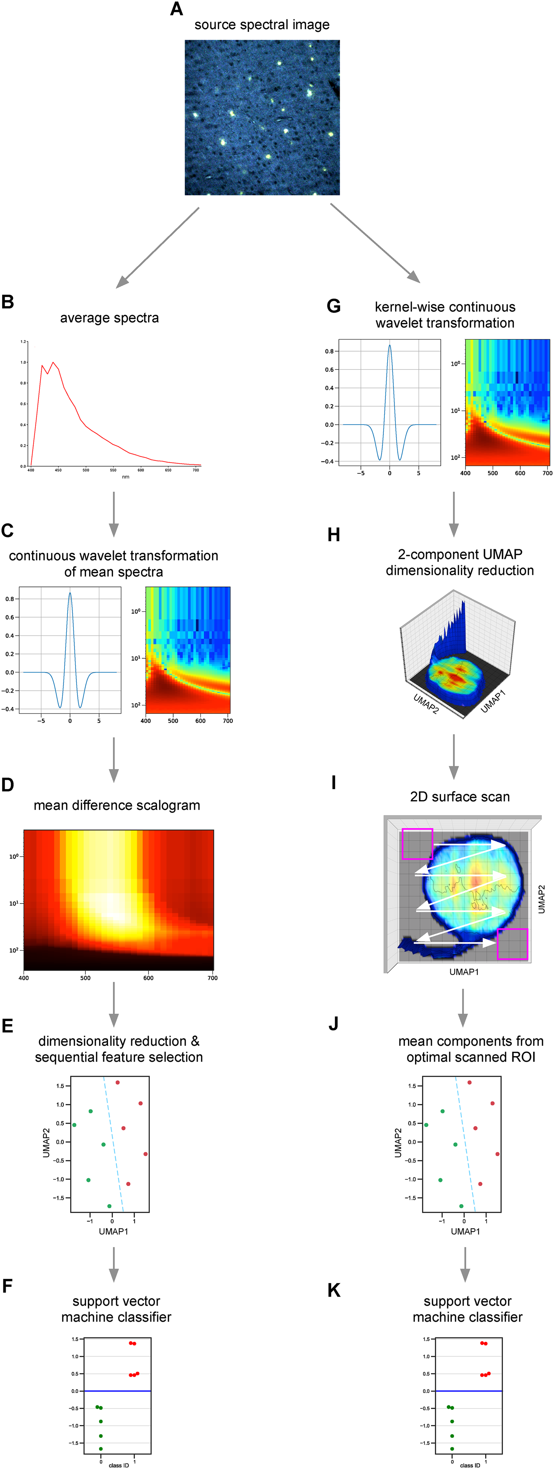
Graphical illustration of the machine learning pipeline used for analysis of spectral images that flowed along 2 paths: track 1 (A-F) and track 2 (G-K). See text for more detailed explanation.

The second track (Figure 1G-K) was used for visual display of spectral distributions within an image, and for identification of subsets of image pixels that might be even more predictive of class membership than all-pixel mean spectra. Once the best wavelet/compression pair was determined using mean spectra from the first track, spectral “kernels” were calculated by averaging 3 × 3 adjacent spectral pixels for denoising and to reduce computational burden. Each averaged kernel was transformed with the best wavelet/compression pair and the kernel-wise scalograms reduced to 2 dimensions using UMAP, then plotted on a surface, with the X and Y axes representing the two UMAP components, the kernel intensity on the Z axis, and the surface color reporting the relative frequency of kernels at each XY position (Figure 1H). In essence, each position along the XY (UMAP1 versus UMAP2) plane reflects a different spectral shape. An unbiased “surface scan” was conducted by rastering a region of interest (ROI) over the 2D UMAP surfaces, mean components calculated for each subject, and the optimal ROI selected that encloses UMAP components that best separate the two groups, determined by minimizing multivariate analysis of variance (MANOVA) p while maximizing the number of included kernels. Once the optimal region was identified, mean UMAP components from all included kernels were calculated and an SVM used to determine a linear decision boundary (Figure 1J,K) as in the first track.

The algorithms were implemented using Python v.3.12 and the following libraries: numpy v1.26.4, pandas v2.0.3, umap v0.5.7, mlxtend (SequentialFeatureSelector) v0.23.4 and scikit-learn v1.5.2. Scripts were run on an Apple Mac Studio with a 24 core M2 Ultra chip and 192 GB RAM. To determine the optimal decision boundary that separated the groups, a grid search was performed using ≈200 different continuous wavelets, 20 compression levels, and a series of C, gamma and kernel type (linear or rbf) hyperparameters for the support vector classifier (SVC). SequentialFeatureSelector was used to select the best components for inter-group differences in an unbiased manner. Wavelet types, compression levels, SequentialFeatureSelector and the SVC were all wrapped in Leave-One-Out cross-validation to reduce data leakage, and cross-validated accuracy used as the first arbiter of best model selection. Models that were tied for cross-validated accuracy were resolved by minimizing the Davies-Bouldin index (a measure of cluster compactness and separation). Because UMAP is inherently non-deterministic (i.e., will yield different results depending on the model's initialization), 5 randomly-initialized UMAP fits were performed for each combination of hyperparameters, and the embeddings averaged. To verify against overfitting, target labels were randomized and the fits repeated. This was done five times and the randomized results averaged, with the expectation that now the classification would fail.

This article does not contain any studies using live human or animal participants.

Results

Fluorescence spectroscopy of 5xFAD mouse brain

Figure 2 shows example spectral micrographs of 9-month-old mouse cortical brain sections stained with the amyloid probe K114. The wild type (WT) sample exhibited a relatively uniform blue hue as did the non-plaque background parenchyma in the 5xFAD sample, with a hue indistinguishable from WT to the naked eye. In addition, the 5xFAD section also showed numerous bright amyloid plaques, expected at this age in this transgenic strain. ²⁹ Figure 2C shows an overlay of normalized spectra from the three regions. K114 exhibits a characteristic doublet at around 425–450 nm when bound to Aβ fibrils.^27,28 Whereas the plaques showed a very prominent broad red-shifted emission peaking at ≈550 nm, characteristic of amyloid-bound probe,^27,35,36 the mean background spectra were otherwise virtually identical in both WT and 5xFAD cortex when viewed as an overlay.

Figure 2.

Spectral differences computed from WT and 5xFAD mouse cortex stained with K114. (A,B) Representative micrographs from WT and 5xFAD brain (respectively) showed a uniform bluish background. In addition, the latter contained numerous bright yellowish amyloid plaques as expected at 9 mo of age. (C) Mean normalized background spectra from WT (green ROI and trace) versus 5xFAD (orange ROI and trace) brain are virtually indistinguishable, whereas plaques showed the characteristic broad peak at around 550 nm. (D) Dimensionality of spectral kernels was reduced from 32 wavelengths to 2 UMAP components, then plotted on a 4D histogram where each position on the UMAP plane represents a different spectral shape, intensity is plotted on the Z axis, and kernel frequency encoded by surface color. Plaque kernels are easily seen as a distinct higher-intensity cluster (arrow). (E) Raw kernel-wise spectra can be decomposed using wavelets, such as the mexh wavelet shown as an example, with the corresponding scalogram representing scale on the Y axis versus wavelength along X. (F) Kernel-wise scalograms were embedded into 2D space using UMAP, and the UMAP component pairs plotted as above. The distributions are different than with raw spectra as the UMAP input, but the spectrally unique plaque cluster is once again clearly apparent (arrow). Scale bars: 50 µm.

Averaging all pixels to generate mean spectra as shown in Figure 2C will not capture potentially important spectral heterogeneities in images, like the striking but infrequent plaque pixels in Figure 2B. To visualize such variations, 3 × 3 pixel kernels were averaged then each 32-element kernel spectrum was reduced to 2 dimensions using UMAP and plotted on a 4D surface as shown in Figure 2D. The higher intensity and spectrally distinct plaque kernels are clearly distinguishable (arrow). Alternatively, using wavelet transformation each kernel spectrum can be individually decomposed into a scalogram, then again dimensionally reduced and plotted on an analogous surface. In the example, a mexh wavelet was used for illustration (Figure 2E), yielding surfaces that are quite different from those obtained using raw spectra, but where the plaque kernels again stand out in a distinct cluster.

Detecting plaques in 5xFAD versus WT is trivial as these deposits are clearly visible in one and not the other, nor is spectral quantitation a challenge since a simple spectral ratio of the intensity above versus below 480 nm for example would be sufficient to distinguish plaque spectra from those of the seemingly normal background. More challenging is a means to distinguish and quantitate potential differences in the background fluorescence that could indicate subtle widespread pathology in the 5xFAD brain. For the mouse brain sections, we adopted the pipeline in track 1 (Figure 1B-F), reducing all pixels from each subject to a single mean spectrum from background regions only. This trade-off implies potentially losing information from small features, in favor of a very large increase in signal-to-noise ratio, while reducing the data volume from millions to a single spectrum for each subject. We tested this approach on the background pixels of the WT and 5XFAD mouse brain images (plaques excluded). A repeat set of images was acquired at higher gain, sacrificing bright plaques many of which were now saturated, in favor of increased signal-to-noise of the dimmer background. A single mean spectrum was computed for each subject and processed using the pipeline outlined in Methods, either using raw mean spectra, or wavelet transformation (≈200 frequency b-spline wavelets were systematically evaluated at 20 different compression levels), as the input to the UMAP reducer. Results are shown in Figure 3. As in Figure 2, the mean background spectra from WT versus 5xFAD samples were nearly identical (Figure 3A). In Figure 3B, raw mean subject-wise spectra were used as the input to the UMAP/SVC pipeline without a wavelet pre-processing step. Neither the 2D UMAP distribution nor the classifier yielded statistically significant differences between the two groups. In contrast, when the same mean spectra were subjected to a pre-processing step using a fbsp1-0.4-0.048 wavelet transformation at a compression of −0.2, followed by the same UMAP/SVC pipeline, now both the 2D distributions and the SVC classifier (C = 15.9, kernel = ’linear’) yielded significant differences (Figure 3C). Randomizing spectral assignments, then re-fitting using the same parameters from the optimal model, failed as expected (Figure 3D). This comparison emphasizes the utility of spectral wavelet decomposition prior to conventional dimensionality reduction and classification steps.

Figure 3.

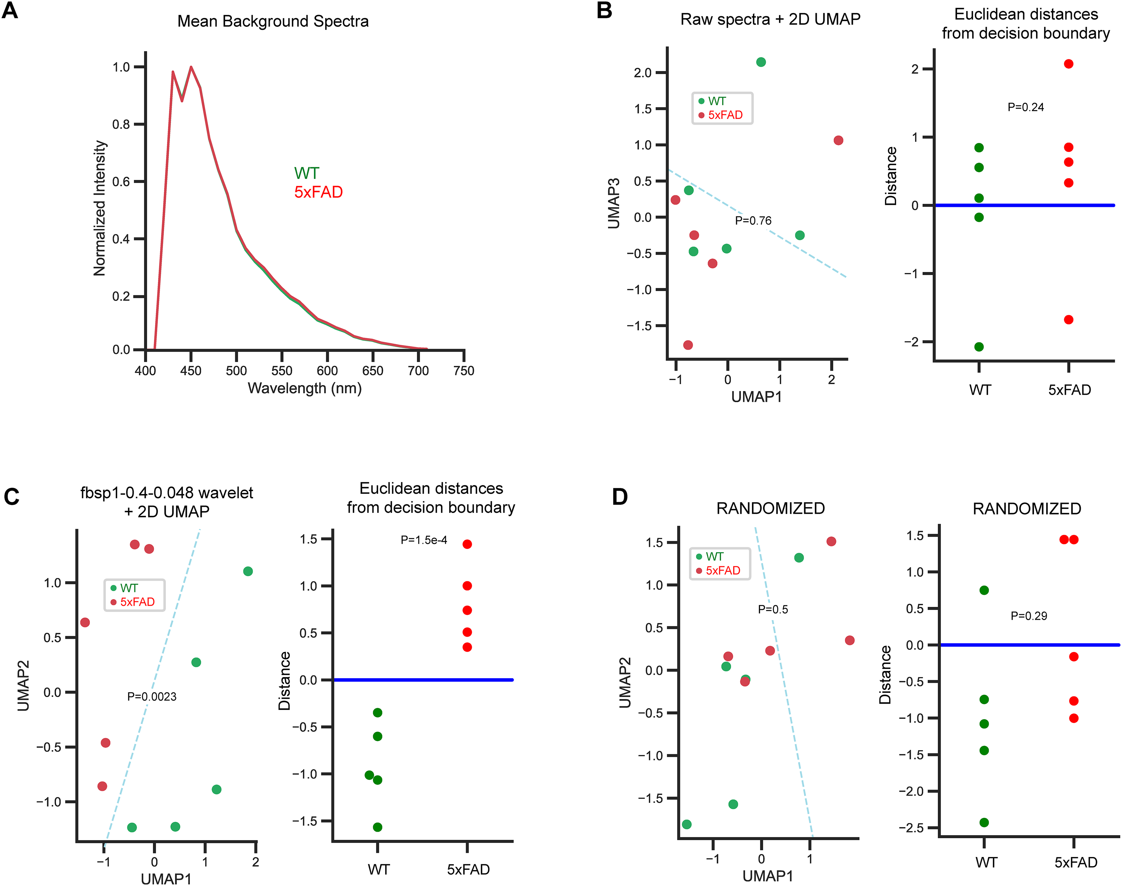
Classification of background signal from WT and 5xFAD mouse brain: comparison of raw mean spectra versus wavelet decomposition. (A) Overall mean background spectra from all mice in each class are very similar when displayed as a simple overlay. (B) Raw mean spectra (a single averaged spectrum for each mouse) were subjected to dimensionality reduction (from 32 wavelength bins to 2 UMAP components) using unsupervised UMAP, then plotted on a 2D scatterplot. The distributions were not different by MANOVA. An SVC was then used to generate the optimal linear decision boundary from the UMAP components and this too failed to find a good solution. (C) When the same mean subject-wise spectra were transformed using a fbsp1-0.4-0.048 wavelet, then passed to the same pipeline, now both the 2D UMAP components and the classification were statistically significant. (D) Repeating the fit with optimized parameters and randomized class assignments caused the model to fail as expected. P values for differences in 2D UMAP components were calculated using multivariate ANOVA, and 1-tailed t-tests were used for differences in Euclidean distances here and in all subsequent figures where appropriate.

Machine learning-based analysis of human PBMC immunoprecipitates

We then examined PBMCs using similar approaches to see if we could detect the AD state from this easily-accessible matrix. Figure 4A and 4B shows representative spectral micrographs of anti-Aβ antibody-coated magnetic beads after incubation with frozen human PBMC homogenates then stained with K114, the same probe used for mouse brain samples. The beads were uniformly blue in both the control and AD groups, with no distinctive features nor any perceptible differences to the naked eye. An overlay of the mean spectra from each group shows them to be visually indistinguishable (Figure 4C). Subject-wise mean spectra were transformed using a cmor3.08-1.26 wavelet which was selected after an unbiased scan of 232 different wavelet functions (Figure 4D). The difference scalogram (Figure 4E) indicates that the largest group differences were located in the 500–600 nm band, and at high signal frequencies (small scales). Subject-wise scalograms were reduced to 3 UMAP components, of which the best 2 were chosen (UMAP2 and 3) by unbiased sequential feature selection. Figure 4F shows the distances from the linear decision boundary from the two mean UMAP components failed to separate classes (p = 0.37, area under the curve (AUC) = 0.56). This indicates that, unlike the background of WT versus 5xFAD mouse cortex, mean spectra from such an immunoprecipitation were not distinct enough for group separation using combined averaged spectra alone.

Figure 4.

Spectral analysis of immunoprecipitates from frozen PBMCs. Immunobeads from a healthy control (HC) (A) and a pathologically confirmed AD case (B) stained with K114 were indistinguishable, appearing uniformly blue (scale bars: 10 µm). (C) The overlay shows that the mean spectra from each class were also visually indistinguishable. (D) Subject-wise mean spectra were transformed using a cmor3.08-1.26 wavelet. (E) Difference scalogram shows greatest group differences in the 500–600 nm band and at smaller scales. F: Reduction of subject-wise mean spectra to two UMAP components and classification using an SVC (track 1, Figure 1B-F) was not capable of distinguishing the two groups. (G,H) Kernelwise UMAP reductions using the optimized wavelet (track 2, Figure 1G-K) and plotted as 2D histograms, with the optimal subpopulation of kernels shown by the white ROI. I: Surface plot showing many statistically significant solutions generated by the surface scan (see text); solutions with p > 0.05 are shown in gray. (J) Using the optimal kernel subpopulation, rather than mean spectra computed from all kernels for each subject, group classification was now successful. (K) Receiver operating curve for data in panel J.

To explore whether there exists a subpopulation of image kernels that could perform better, the optimal cmor3.08-1.26 wavelet was used to decompose each spectral kernel (rather than subject-wise mean spectra) in all control and AD bead images as the initial step along the track 2 analysis (Figure 1G-K). Mean surfaces from these kernel-wise decompositions are shown in Figure 4G and 4H, with the optimal ROI after an unbiased surface scan shown enclosing the subpopulation of kernels that best separated control from AD. Of note, while the optimal ROI is shown, there exist many statistically significant solutions as illustrated in Figure 4I. Interestingly, these solutions occupied a “rim” at the periphery of the kernel clusters, a location of highest intensity (not shown); this is likely not a coincidence because K114 is well known both to shift spectrum and increase brightness when labeling fibrillar amyloid.^27,28 The mean UMAP components from the optimal subpopulation were now strongly statistically different in the 2D plane (p = 7.5e-4), as were the boundary distances (p = 6.1e-5, AUC = 0.95; optimal SVC hyperparameters: C = 19.3, kernel = 'linear’; Figure 4J). The swarmplot shows all experiments as individual markers. Because all subjects were analyzed twice on separate occasions, the subject-wise averaged distance and associated statistics are shown in Supplemental Figure 1. The groups remained statistically different (Mann-Whitney U p = 1.1e-3) and the AUC improved to 1.0 showing complete separation.

Having shown that K114 spectra from PBMC immunoprecipitates can effectively distinguish between healthy control and AD samples after scanning for an optimal kernel sub-population, we then explored whether this spectral information could predict brain histopathology obtained at post-mortem examination. We used the sum of the raw semiquantitative Braak score for neurofibrillary tangle pathology (B) + the Consortium to Establish a Registry for Alzheimer's Disease (CERAD) score for neuritic plaque pathology ³⁷ as the continuous target variable (‘B + C’). The same subject-wise mean UMAP components identified by the optimal ROI (Figure 4G-1) were used as the training vectors for the regressor. StratifiedKFold cross-validation was used with 5 splits to limit over-fitting, a radial basis function kernel for the support vector regressor and a grid search of hyperparameters. Figure 5 shows that our model achieved a very good ability to predict neuropathology scores from PBMC spectra (R = 0.89; optimal wavelet: fbsp2-0.18-0.036, compression: 0.73).

Figure 5.

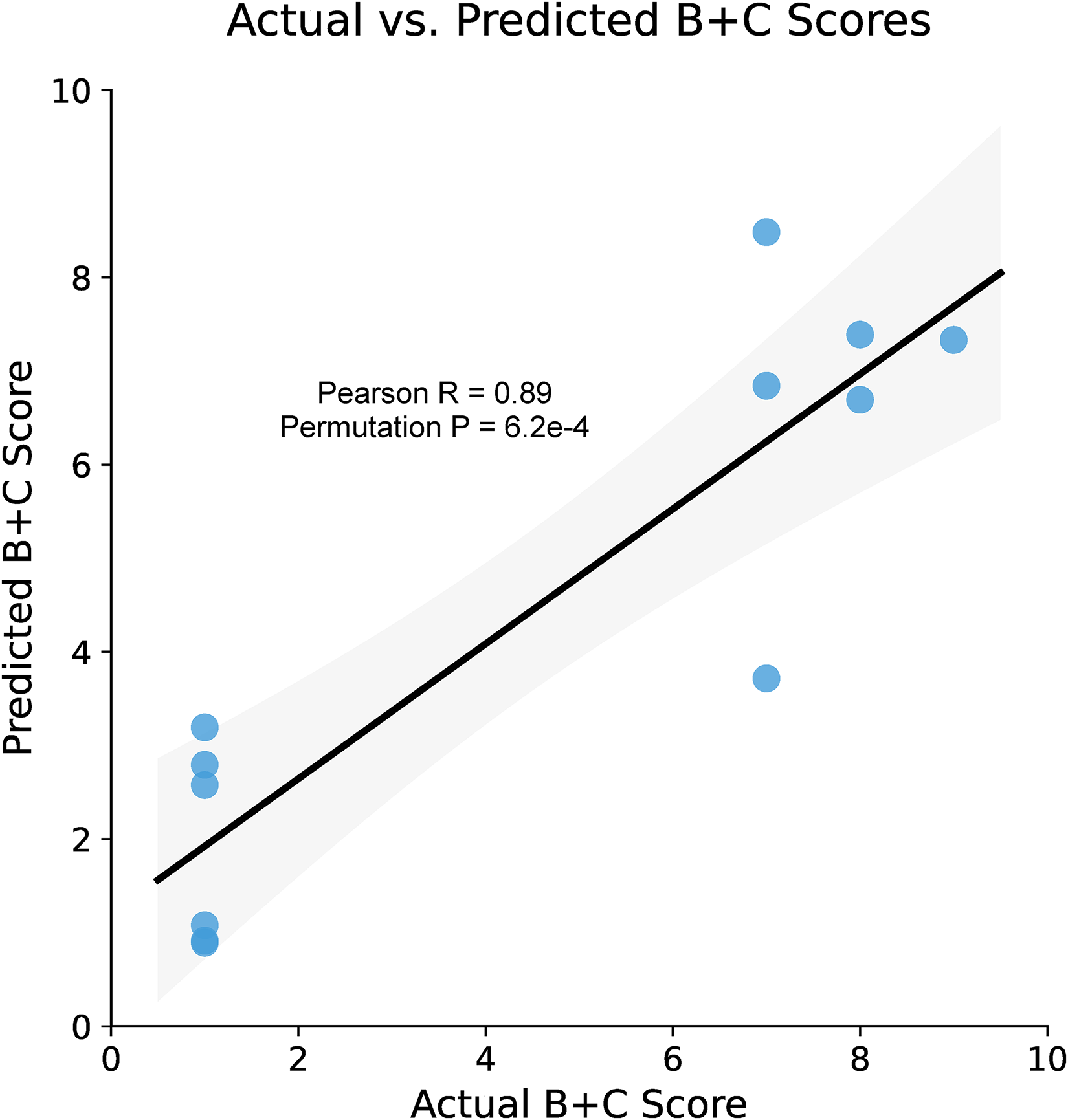
Prediction of brain neuropathology from PBMC spectral data. Optimal components identified by unbiased surface scans of UMAP-reduced spectra (Figure 4G-1) were used as input to a Support Vector Regressor, with the combined B + C neuropathological scores as the target variable. The neuropathological scores predicted by our model from PBMC spectral data were strongly correlated with the actual neuropathological scores. 95% confidence band shown in gray. Each point represents an average of two experiments from each subject.

Discussion

Protein misfolding is a ubiquitous phenomenon in most if not all neurodegenerative disorders, resulting in aggregation of monomeric proteins or peptides into a broad range of higher order assemblies ranging from oligomers to fibrils. These may go on to coalesce into larger insoluble deposits visible by light microscopy (e.g., neuritic plaques, neurofibrillary tangles, Lewy bodies) and form the foundation of histopathological diagnosis of various neurodegenerative diseases.^6,7,38 Identification of such larger deposits is straightforward using well-established histological stains or immunohistochemistry. These are also well visualized using a variety of fluorescent probes (e.g., Figure 2B).^15,17,22,39 More challenging is detection of less mature aggregates that have not condensed into a morphologically distinguishable deposit, and can easily be discounted as background staining noise. These species may be as important as the readily visible deposits because oligomeric species are thought to be more toxic and therefore might be more directly involved in disease progression^40–42; may indicate a more widespread involvement of the CNS; and likely appear sooner in the disease process and therefore could aid in earlier diagnosis.

An interesting and very useful property of many small-molecule fluorescent amyloid dyes is their propensity to change emission spectrum when contacting various amyloid assemblies,^22,39,43 with a number of Congo Red derivatives (e.g., K114, BSB, X-34) exhibiting such amyloid-dependent spectral shifts.^36,44–46 We reasoned that measuring spectral changes of such dyes, rather than fluorescence intensity (which is harder to control and reproduce), could be a more reliable method of detecting and quantitating presence of β sheet-rich misfolded protein aggregates in cells and tissues. We selected K114, a high-affinity amyloid probe, because of its brightness and robust spectral shifts when bound to amyloid fibrils and plaques in AD tissue.^35,47 Spectral confocal microscopy allowed the collection of complete 32-channel spectra from each pixel in an image. To validate and optimize our methods, we first used sections of cortex from 9-month-old 5xFAD AD mice, a strain known to predictably accumulate amyloid pathology with age.^29,47 As illustrated in Figure 2, K114 brightly labeled amyloid plaques in these samples given the known accumulation of robust plaque pathology at this age. Compared to the bluish hue of the K114-labeled background parenchyma, plaques exhibited a prominent additional peak at ≈550 nm (Figure 2C), a characteristic spectral shift when this dye is bound to Aβ fibrils. ²⁷ In contrast, spectral differences in the non-plaque background were barely apparent when compared on an average basis. Importantly, emission spectrum of K114 may shift differently depending on the type of amyloid examined, ⁴⁸ making the amyloid-driven change of emission spectrum challenging to predict. For this reason, we turned to unbiased machine learning methods to detect and classify spectral changes in healthy versus diseased samples. Spectral images are inherently high-dimensional presenting challenges for visualization, interpretation and analysis. We used UMAP manifold embedding that maintains both local and global data structures ³² to project the spectral data into a lower dimensional space. Figure 2D shows an example of spectral imaging data from WT and 5xFAD mouse brain stained with K114, reduced to two UMAP components and displayed as a 4D histogram. Such plots show the spectral heterogeneity in the images, in effect distributing different spectral shapes across the 2D UMAP plane. The high intensity, and spectrally unique, plaque pixels were clearly visualized as a separate cluster. Notably, rather than having discretely different spectra, the plaques exhibited a continuum of spectral shapes extending from one region of the background distribution towards a final spectrally distinct high-intensity cluster representing the brightest plaque cores. This likely reflects variations in nanostructure of the constituent amyloid deposits, suggesting a continuum of amyloid structure from normal-appearing background, to plaque periphery, to plaque core.

In contrast to periodic signals such as sound or radio-frequency waves, spectra are inherently non-stationary in that their frequency content varies by position along the horizontal wavelength axis. The K114 spectra in Figure 2C illustrate this, with higher frequency components in the doublet located around 425–450 nm, and lower frequencies (more gradual changes in the spectrum) at longer wavelengths. Inputting raw spectra into machine learning pipelines may fail to capture subtle features of such signals, especially if low amplitude components at any given frequency band are the most discriminative. Wavelet transformation is a mathematical method particularly well suited for processing non-stationary signals, and unlike Fourier analysis, will decompose a series along both frequency (“scale”) and time (in our case “wavelength”) axes. This now allows examination of frequency components at each wavelength. Figure 2E shows an example transformation of spectra from mouse brain using a mexh wavelet yielding a 50 element high (scales) × 32 element wide (wavelengths) “image”. Now the many powerful machine learning methods for image analysis and classification can be applied. Figure 2F shows an example of reduction of mouse brain spectral data from 1600 (50 × 32) to 2 dimensions and plotted as for raw spectra in Figure 2D. While the kernel distributions along the surface are different than raw spectral reductions (Figure 2D), once again the plaque cluster is readily apparent.

A significant challenge with spectral imaging and analysis is the sheer volume of data, consisting of millions of spectral pixels containing both spatial (XY) and spectral information; training on such large data sets is often computationally impractical. Instead, we opted to greatly reduce the amount of data by computing a single average spectrum from all spectral pixels in all images, for each subject. The potential disadvantage of mean spectral analysis is that infrequent features, such as the very distinctive but infrequent plaque regions in the 5xFAD brain sections, might be diluted by more prevalent, but potentially uninformative features from the remainder of the image. However, averaging greatly reduces noise in the spectra, potentially aiding training of models. It turns out that for some datasets a single low-noise averaged spectrum per subject is sufficient for training models and gaining important insight into samples as illustrated in Figure 3. Here we isolated background regions only (excluding plaques) from WT and 5xFAD brain images (excluding plaques from the latter) and computed a single mean spectrum from each subject. When such raw spectral data were used for classification this was not successful (Figure 3). However, a pre-processing step using wavelet decomposition, followed by UMAP dimensionality reduction, and a final SVM classification step yielded superior results (Figure 3C), underscoring the utility of wavelet decomposition to extract subtle but informative spectral features. An important component of the wavelet pre-processing step included application of a series of compression levels to the scalograms which has the effect of numerically varying the relative contributions of weak versus strong regions (Figure 2E). Since we could not know a priori which scale or wavelength position would be most important for optimal classification, a range of compression levels was tested in an unbiased manner and was included as a tunable parameter in the cross-validation. Note that only the final step in the pipeline is supervised, such that the 2D UMAP distributions are agnostic to the WT versus 5xFAD classes. From this analysis we were able to conclude that despite its normal histological appearance, the normal-appearing cortex was likely affected by subtle amyloid deposition in 5xFAD mice, and that the plaques are just the tip of the iceberg in what is likely widespread brain pathology in these animals.^21,49

Having validated that our method is able to detect subtle amyloid-driven spectral changes using standardized mouse brain samples, we then turned our attention to immunoprecipitates of human PBMCs to see if healthy control and AD subjects could be distinguished using the same principles. This goal was the most challenging as the mean spectra were visually indistinguishable as shown in Figure 4C, indicating that numerical differences that might support reliable classification would be very subtle. With these samples, relying on a single mean spectrum per subject was not successful (Figure 4F). Instead, we calculated kernel-wise scalograms from all spectral images which were reduced to 2 dimensions using UMAP, then systematically scanned to determine an optimal subpopulation of kernels that was capable of correctly classifying the subjects (white ROI in Figure 4G,H; swarmplot in J). Together this indicates that unlike more severely affected mouse cortex, immuno-extracts from circulating human PBMCs contained much lower amounts of disease-associated material, that could nonetheless be detected by more sophisticated numerical methods designed to isolate a subpopulation of spectral pixels that can better discriminate between groups, yielding a final AUC of 0.95 that rivals currently available plasma assays. ⁵⁰ Of note, different wavelets/compressions were found to be optimal for the mouse brain versus PBMC samples, underscoring how matching wavelet functions to the shapes of the subject spectra was important for optimal performance. Moreover, while we chose Leave-One-Out and StratifiedKFold cross-validation strategies to limit overfitting, other methods could also be applied including bootstrapping and external validation with larger sample sizes.

Equally intriguing was the ability of the PBMC-derived spectral data and regression model to predict AD neuropathology, with an excellent correlation between actual and predicted B + C scores of 0.89 (Figure 5). A likely source of the disease-reporting material captured by our immunobeads is lysosomes known to accumulate pathological debris for degradation. ⁵¹ Given that amyloids are generally resistant to proteases,^52,53 it is possible that AD-related material was phagocytosed by these cells, could not be completely degraded, and remained trapped in lysosomes, ⁵⁴ then could be recovered by immunoprecipitation of sonicated frozen PBMCs. Given the success of spectral shifts from PBMCs in paralleling not only clinical diagnosis but brain pathology, it appears that after ingestion by PBMCs amyloid conformations were preserved enough to modulate K114 fluorescence for reliable reporting. It should be noted that this correlation is preliminary given the limited sample size and the relative “coarseness” and semiquantitative nature of the Braak and CERAD scores but, nevertheless, lends support to the notion that circulating blood elements may reflect brain pathology to a significant degree.

CSF assays of Aβ₄₀, Aβ₄₂, tau, and p-tau, together with amyloid and tau-positron emission tomography (PET), have been shown to be good predictors of AD pathology.^55–59 A number of AD plasma biomarkers have been reported in recent years, with immunoassays for tau phosphorylated at various threonines emerging as reliable reporters of brain Aβ and tau positivity with AUCs exceeding 0.9.^60–64 Limitations of our report include the relatively small sample size, as our intention was a proof-of-principle study to showcase potential and robustness of fluorescence spectroscopy-based approaches. In addition, while a direct comparison with current plasma biomarkers would have been instructive, unfortunately this matching information was not available for the PBMC samples procured. However, the robust correlation with brain neuropathology (Figure 5) gives confidence that our method is a reliable predictor of the actual AD pathological state. Although creating clinically-applicable predictive models will require larger samples sizes, our technique exhibits performance comparable to latest generation plasma biomarkers. A number of techniques also use fluorescence as a detection method generally employing Forster resonance energy transfer, intensity changes of amyloid-sensitive probes such as thioflavin-T, fluorescent labeling of peptide substrates, surface plasmon resonance, and Raman spectroscopy methods, to name a few (reviews^17,65:). Invariably these approaches aim to quantitatively detect concentrations of relevant proteins and peptides with high sensitivity, without regard to their conformations or higher-order aggregation that are potentially relevant to disease progression. One area where a spectral assay may hold advantage over quantitative measures of various proteins or their phosphoforms, which are agnostic to higher order aggregate structure, might be the ability to report “strains” of pathological morphotypes. For instance, fluorescent amyloid probes are known to emit different spectra when bound to different amyloids, such as parenchymal AD plaques versus cerebral amyloid angiopathy-related vascular amyloid.^28,47 This could partially overcome the non-specific nature of amyloid probe reporting, i.e., although K114 labels not only amyloids composed of Aβ, unique spectral signatures from other types of fibrils could be distinguishable. Further studies including other neurodegenerative diseases will be required to establish this. With the advent of amyloid-clearing immunotherapies, and their occasional serious side effects that seem to be related to vascular amyloid,^66,67 using machine learning and spectral interrogation of blood elements, it may be possible to train models to predict presence of vascular amyloid and risk-stratify therapies. We have evidence of different spectral signatures from AD plaque deposits in normally-aged brains versus those with cognitive decline ante-mortem (Stepanchuk and Stys, manuscript under review). ⁶⁸ This raises the intriguing possibility of benign versus more aggressive amyloid strains that underpin clinical disability. If such signatures are reflected in blood elements, more sophisticated models using larger datasets could potentially be trained to distinguish subjects with benign amyloid accumulation not requiring therapy, from those whose clinical course is predicted to be unfavorable, and in whom the benefits of disease-modifying therapies would outweigh the risks.

Supplemental Material

sj-docx-1-alz-10.1177_13872877261453512 - Supplemental material for Fluorescence spectroscopy and machine learning methods for detection of Alzheimer's disease from circulating white blood cells

Supplemental material, sj-docx-1-alz-10.1177_13872877261453512 for Fluorescence spectroscopy and machine learning methods for detection of Alzheimer's disease from circulating white blood cells by Shigeki Tsutsui, Anastasiia A. Stepanchuk, Julian P. Stys, Stefanie A. G. Black, George W. Templeton, Russell Greiner and Peter K. Stys in Journal of Alzheimer's Disease