
Abstract
At microwave frequencies, the electromagnetic (EM) characterization of materials is not possible through direct measurements. In this case, the Nicholson-Ross-Weir (NRW) algorithm is the standard phenomenological analytical approach for the inverse problem. The algorithm finds the equivalent complex permittivity and permeability, starting from scattering parameters at two terminals of a waveguide structure containing the material. To be successful, NRW needs a material sample thin enough, and careful operations with complex valued logarithm. When successful, extracted parameters have round-off errors, but when not, the results are wrong. Thus, the inverse problem of the EM material characterization at microwave frequencies is an interesting benchmark for optimization algorithms and machine learning alternatives. A neural network alternative is investigated in this paper for the case of non-magnetic materials, operating at a fixed frequency. This is a necessary first step before approaching neural network (NN) models valid for whole frequency ranges and magneto-dielectric materials. A feed forward NN with one hidden layer was used, its hyperparameters being tuned by employing a multi-objective optimization procedure. Numerical results show that a NN carefully chosen can provide accurate results for a relatively large domain of complex permittivity components, being successful in areas where NRW fails. The implementation, carried out in python with Optuna module, is available for free download.
Keywords
Introduction
The inverse problems in engineering can be seen as strategies searching for approximations of corresponding inverse functions or operators. Function approximation is also one of the possible learning tasks for neural networks (NNs). 1 NNs excel at approximating non-linear functions and learning complex mappings from data, making them well-suited for tasks where traditional algorithms struggle. One such algorithm is the Nicholson-Ross-Weir (NRW) computational method, for the extraction of electromagnetic (EM) material properties at high frequencies proposed in.2,3
In this paper we investigate the use of NNs to solve the inverse problem of finding frequency dependent EM material properties, starting from a known frequency dependent terminal behavior. This is useful for EM characterization of materials at microwave frequency, where direct characterization from measurements is not possible. This is useful in technological advances where new materials and composites are devised for various applications in microwave engineering, such as antennas, sensors, tags,
4
materials for EM shielding,
5
etc). Among the determination methods that exist, the class based on the transmission/reflection (TR) measurements are widely used. A detailed review of TR based methods can be found e.g. in4,6 and references therein. The NRW algorithm belongs to this class of methods, and it is considered a standard approach. NRW extracts material properties assuming the material is homogeneous, isotropic and the EM field propagates according to the transversal electric TE10 mode. To be successful, NRW needs that the material under test (MUT) sample be thin enough. Moreover, careful evaluation of the logarithm function applied to complex numbers must be implemented.
7
Improvements of the standard NRW algorithm were proposed so that to diminish the effect of uncertainties in measurements.8,9 Other modes of propagation (e.g. TM11) for microwave measurements were recently investigated.
10
There is thus a high interest in material characterization at microwave frequency.
11
Finding an alternative for NRW is a good benchmark to start with, before investigating the characterization of anisotropic materials or other modes of propagation. The idea of using NNs for EM characterization of materials was also investigated in
12
, where two separate multi-layer perceptron (MLP) NNs with one hidden layer having 10 neurons each have been used, one having as output
Problem formulation
The NRW computational method starts from the scattering (S) parameters for a material sample assumed homogeneous and isotropic, inserted into a rectangular waveguide through which the TE10 mode of propagation occurs (Figure 1). The method is based on closed form relationships that give the complex permittivity
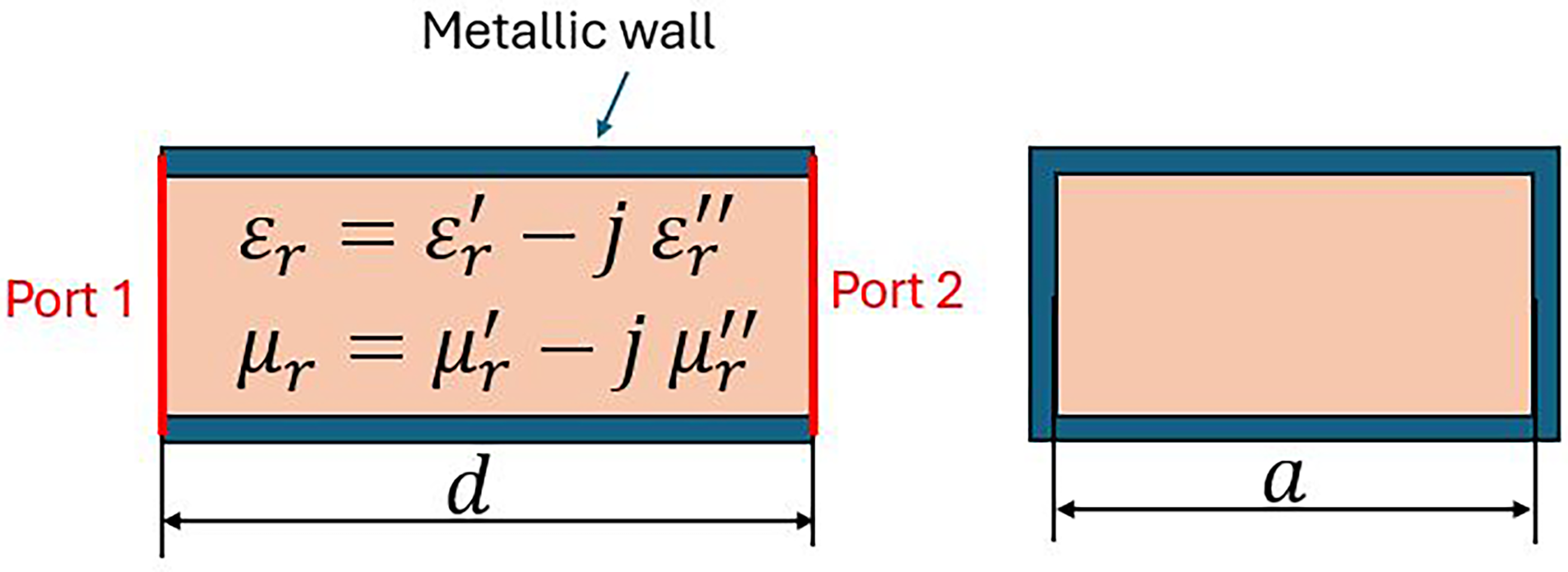
Geometrical model for the NRW procedure: rectangular waveguide, of length d, and width a, filled with a homogenous and isotropic material. Physical model: full-wave EM field, TE10 mode of propagation, PEC conditions on the lateral surface except for two waveguide ports.
It is useful to recall the direct problem, which is stated as follows.
Given: the width of the waveguide a, the thickness of the material sample d, the complex material properties (they can be frequency dependent, losses are included in the imaginary parts) – the permittivity
The direct problem admits the following analytical solution.
7
Let us denote by:
The inverse problem is formulated as follows.
Given: the width of the waveguide a, the thickness of the material sample d, the scattering parameters
The NRW computation is based on the analytical formulas above, written in a way that led to the material properties. The computation is carried out independently for each frequency sample in the chosen frequency range. The algorithm is as follows.
One sensitive part of the algorithm is Step 1, where numerical instabilities are expected if
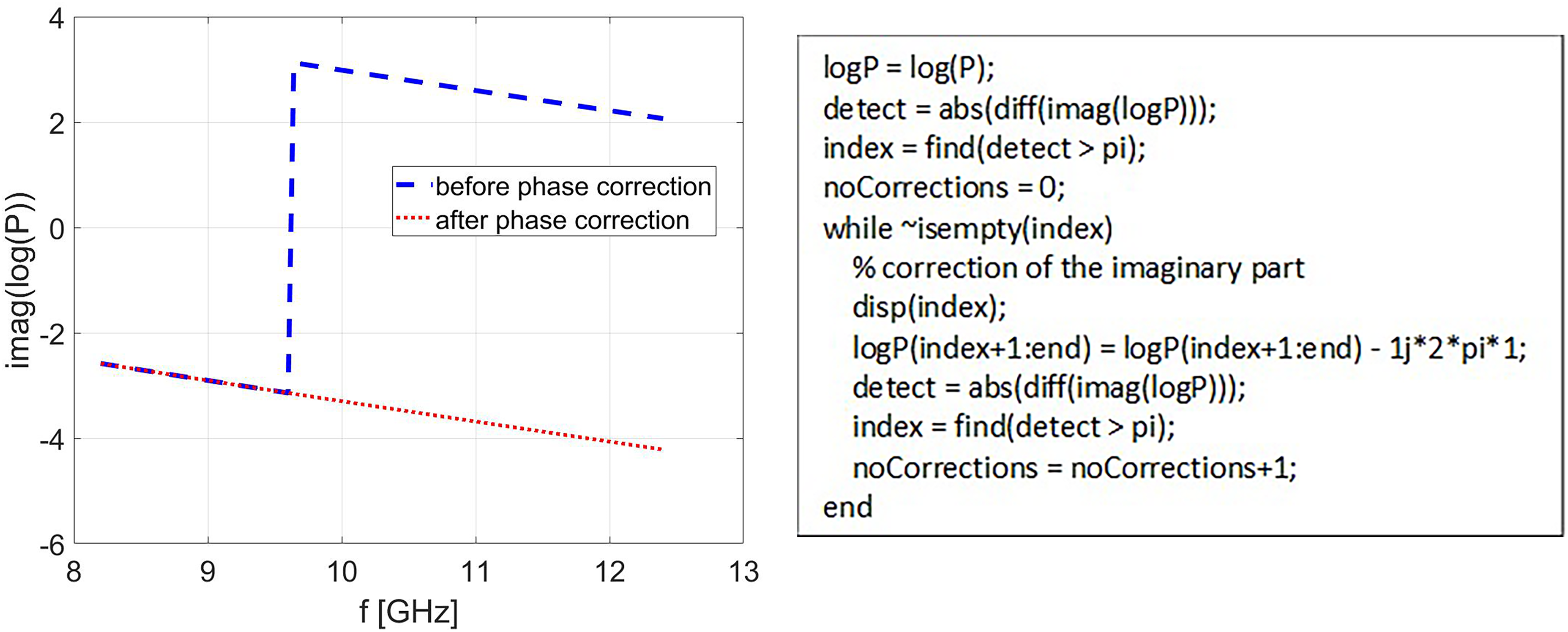
If the logarithm of the first frequency in the frequency range is correct, then phase jumps for the next frequencies can be corrected if needed (MATLAB code is shown on the right).
Let us now consider the frequency fixed at its minimum value, consider a sample with
The permittivity domain
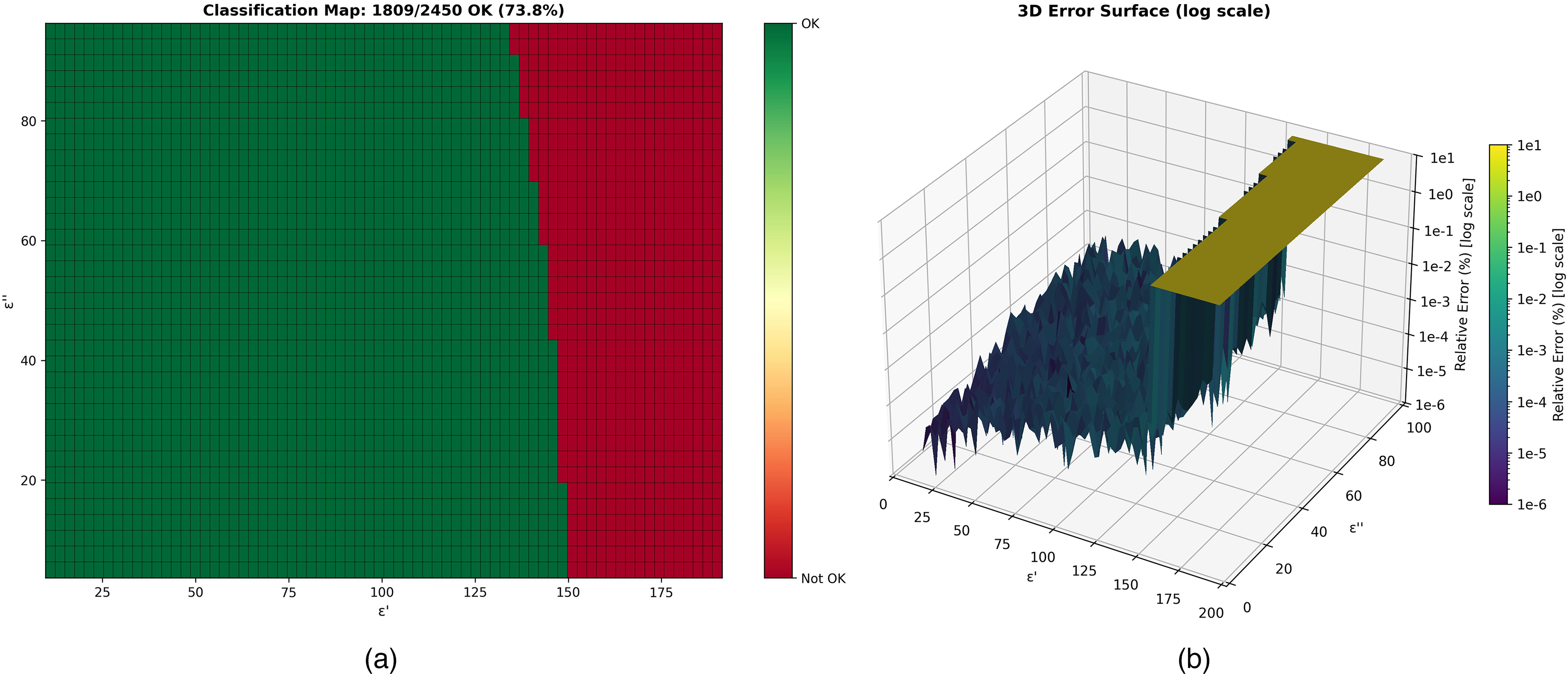
Testing NRW for a fixed frequency f = 8.2 GHz. (a) Materials corresponding to points in the “OK” region led to successful computation, the “Not OK” region corresponds to NRW failures; (b) relative errors that correspond to successful points are round-off errors, in the failure zone the relative errors are over 100%.
NN-MLP based approximation
MLP are a class of feedforward artificial neural networks that have been widely used for function approximation, classification, and regression tasks. A MLP consists of an input layer, one or more hidden layers, and an output layer, each layer being fully connected to the subsequent layer. The universal approximation theorem demonstrates that a MLP with a single hidden layer can approximate any continuous function to arbitrary accuracy, given enough neurons.
14
That is why, in the context of material property extraction we will consider a MLP with one hidden layer, with 4 inputs (the real and imaginary parts of the scattering parameters
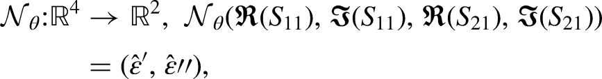
Network architecture 4-H-2
The network consists of one single hidden layer containing H neurons (also known as the width of the layer). The input vector

Data generation and preprocessing
Training data is generated synthetically using the robust EM forward model described in Section 2, ensuring noise-free ground truth labels. The permittivity domain covers
Description of the training, validation, and test datasets, including grid size, number of samples, offsets, and their respective purposes.
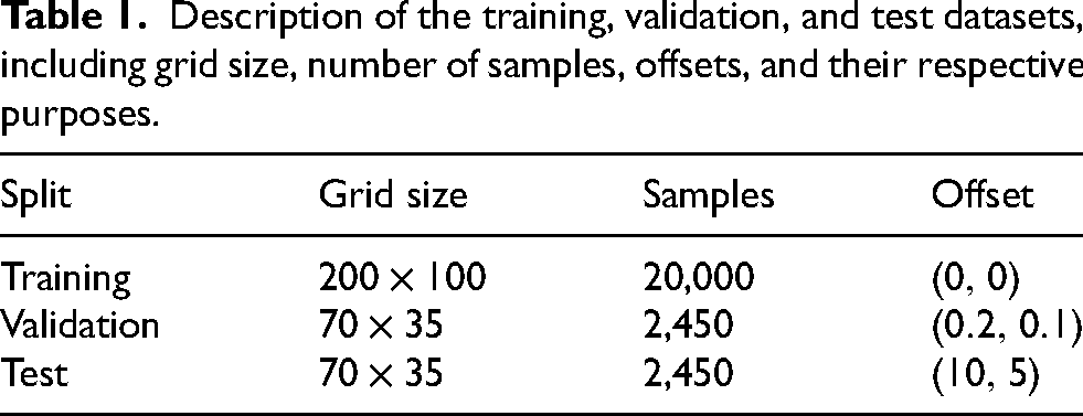
Given that the permittivity values span two orders of magnitude, numerical stability is enforced via z-score standardization applied to both inputs and targets.
18
The standardized value
Training and backpropagation
The training phase is formulated as a global optimization problem where the objective is to minimize a scalar loss function, 
In this formulation: Forward Propagation. A batch of input vectors is propagated through the network's layers. The input is successively transformed by the current parameters (weights and biases) and non-linear activation functions to generate the predicted output Loss Evaluation. A generic loss function Backward Propagation. The sensitivity of the loss with respect to each trainable parameter is computed using the chain rule of calculus. This step calculates the gradient vector Parameter Update. The network parameters are updated using a specific optimization algorithm
Hyperparameters optimization
The performance of neural networks is critically dependent on the selection of hyperparameters, where suboptimal choices can lead to poor convergence or overfitting. Manual tuning of these parameters is often inefficient and may fail to uncover the optimal configuration. To systematically explore the configuration space, we employed Optuna,
20
an automated hyperparameter optimization framework. We defined a comprehensive search space encompassing both architectural and training parameters. Rather than optimizing a single metric, we formulated a bi-objective problem to balance predictive performance against MLP architecture complexity. Let
Architectural Parameters determine the capacity and nonlinearity of the neural network. Hidden Width (
Optimization Parameters control the gradient descent process and loss landscape navigation. Optimizer
We define two competing objective functions: 1. Maximize Strict Accuracy (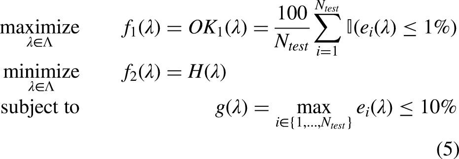
where: 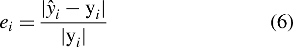
The optimization was conducted using the NSGA-II, 28 which efficiently explores multi-objective spaces by maintaining a population of diverse solutions. To ensure practical utility, we imposed a hard feasibility constraint: any trial yielding a maximum per-sample error exceeding 10% was marked as infeasible and excluded from consideration.
Numerical results
The NN described above was implemented in python with the Optuna module and it is available at https://github.com/bumbeneciconstantinbogdan/S-Param-Inversion, together with the database used for training, validation and testing.
The experimental evaluation assesses the efficacy of the proposed neural network approach against the classical NRW algorithm. The results are derived from a comprehensive hyperparameter study comprising 10,000 trials, of which 6,104 (61.0%) satisfied the feasibility constraint of keeping maximum errors below 10%. The multi-objective optimization identified a Pareto front shown in Figure 4, consisting of four non-dominated configurations, representing the optimal trade-offs between model size (
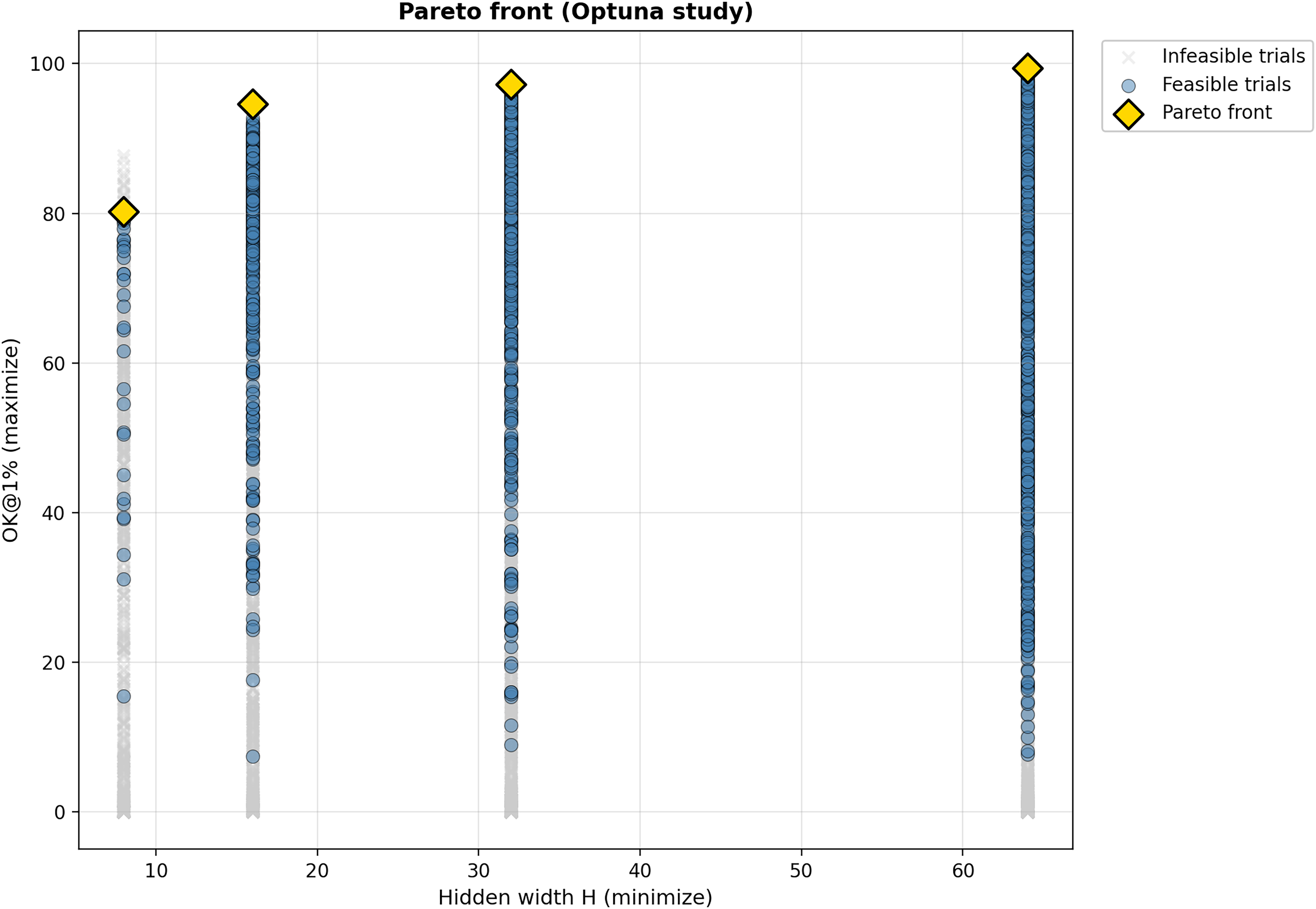
The Pareto front illustrates a steep efficiency curve that flattens rapidly. Upgrading from an ultra-compact
Based on this, we distinguish three deployment tiers: Ultra-Low Resource (
Optimum analysis
While the
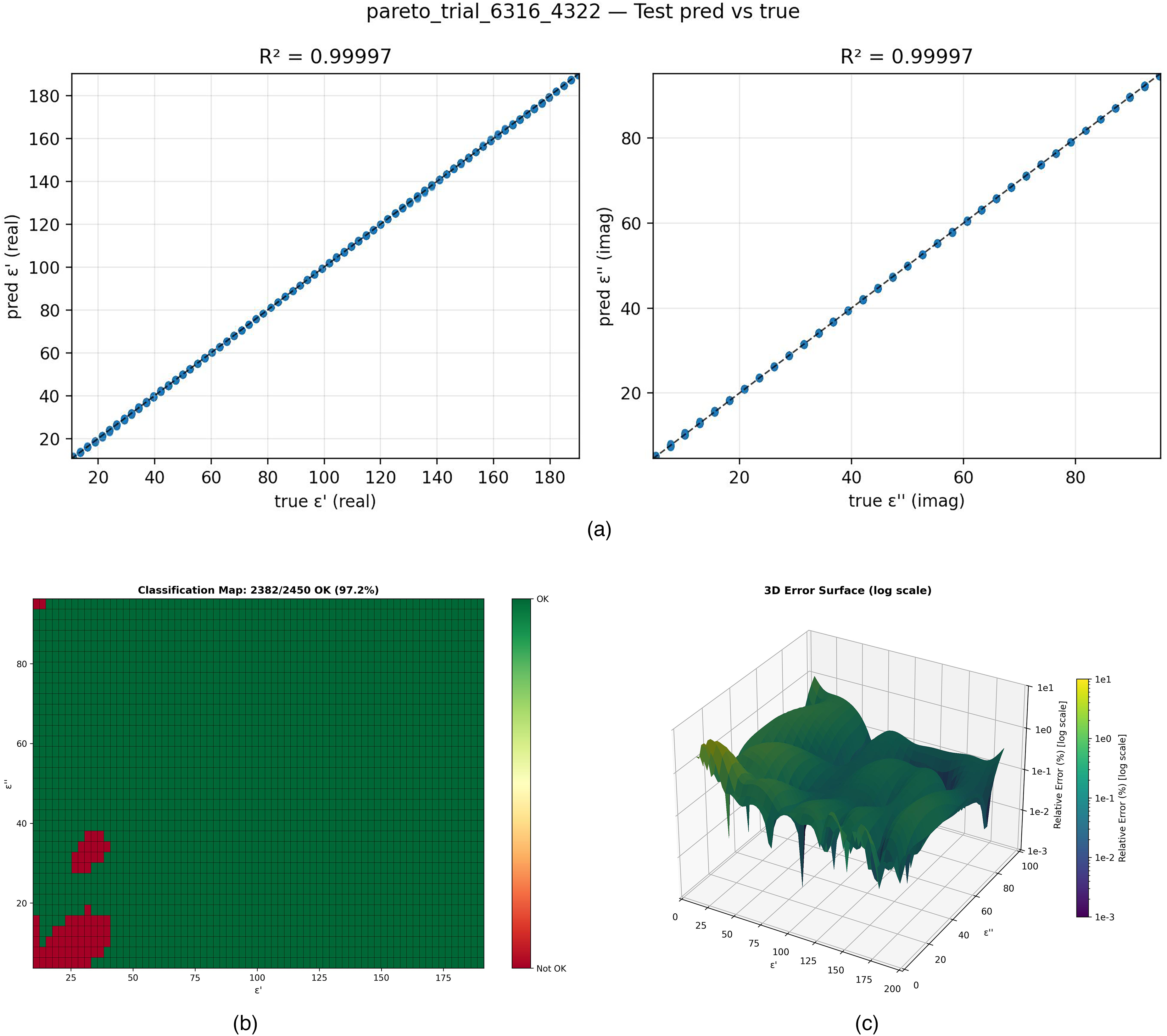
Accuracy assessment for the network configuration. (a) Scatter plots demonstrating the high correlation between predicted and true permittivity values; (b) Classification map quantifying the distribution of samples exceeding the 1% error threshold; (c) 3D relief map visualizing the magnitude of relative errors across the domain.
Hyperparameters final values
The systematic search done with Optuna identified a consistent “recipe” for success shared across the top-performing models. This consensus configuration provides a robust template for training regression networks in this domain, being summarized in Table 2. The search for 10,000 trials was distributed across 8 parallel processes on a 14 inch MacBook (M4 Pro, 24GB Ram). Accounting for process synchronization locks and varying convergence times, the total wall-clock time was approximately 7 h. The average execution time for a single optimization trial was however approximately 13 s, and the typical loss variation during the epochs is shown in Figure 6.
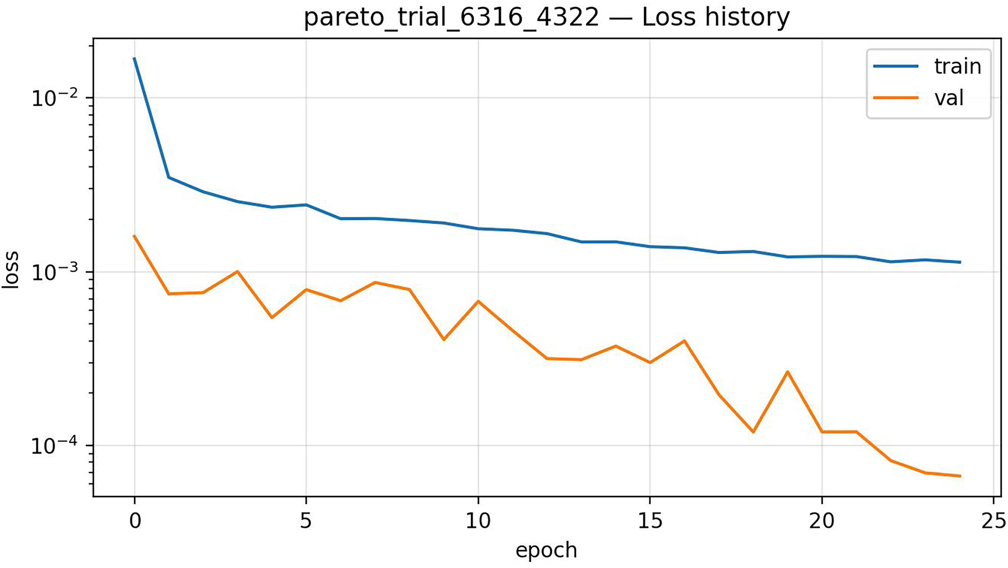
Typical variation of the loss for one single trial, during hyperparameter optimization.
Summary of the optimal training components and hyperparameters used in the model.
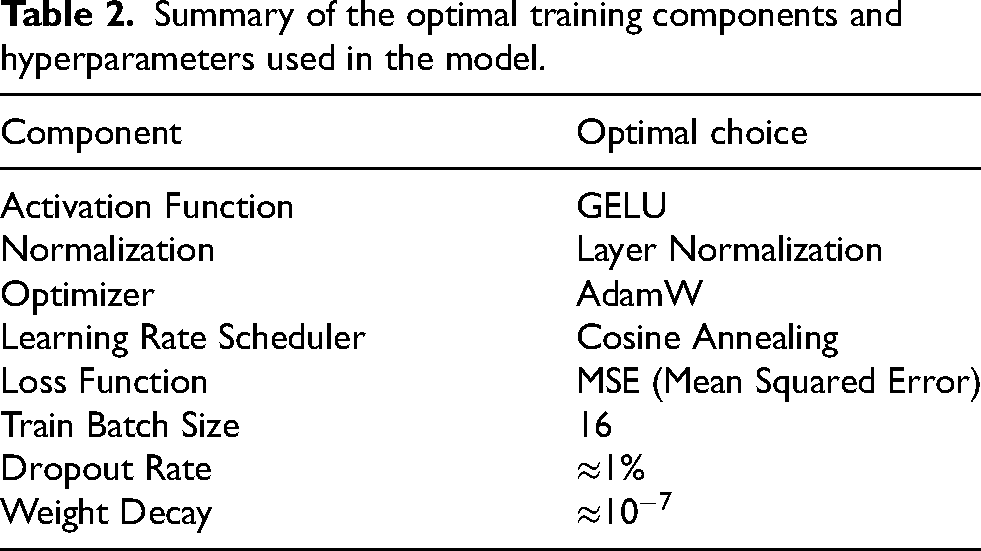
The preference for GELU activation and Layer Normalization was particularly strong, appearing in all Pareto-optimal trials. This consistency suggests that the smooth non-linearity of the GELU function, which avoids the vanishing gradient issues often encountered with standard ReLUs, is essential for accurately approximating the continuous physical mapping of complex permittivity. Furthermore, the dominance of Layer Normalization in the sensitivity analysis indicates that stabilizing activations on a per-sample basis is far more effective than batch-dependent methods for this specific inverse problem.
To understand the drivers of model performance, we conducted a sensitivity analysis using the fANOVA framework. 29 The result is shown in Figure 7.
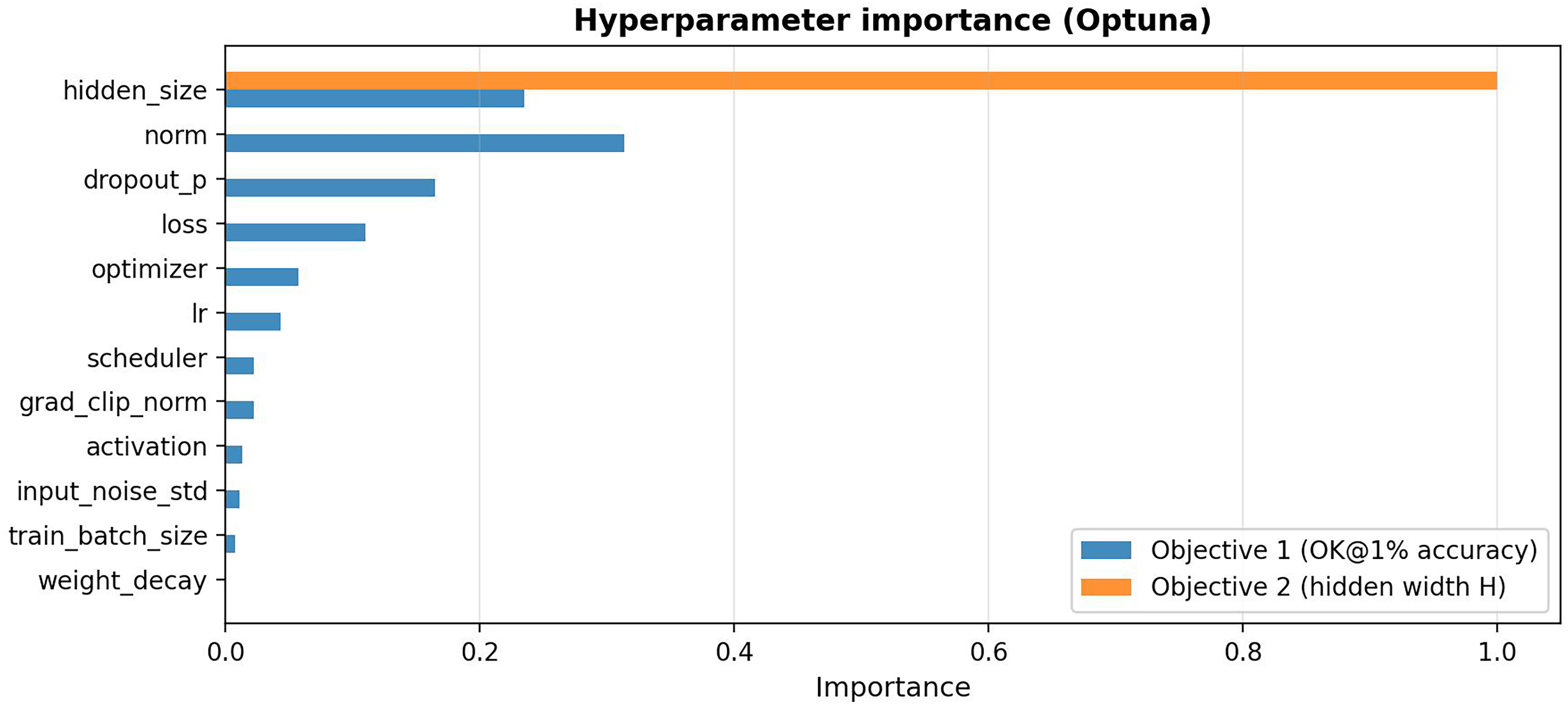
The analysis reveals that layer normalization is the single most important factor for achieving high accuracy, followed by network capacity (hidden size) and dropout regularization. Learning rate and weight decay, often considered critical, show relatively low importance—suggesting the optimal ranges are broad and robust.
Conclusions
This paper proposes a methodology based on NN to replace the standard NRW computational algorithm in case of non-magnetic, isotropic materials. Our methodology uses a feed forward network to find a good approximation of the dependency between the input – the S parameters (2 complex numbers) and the output – the components of the complex permittivity. The chosen architecture for the NN was a MLP with one hidden layer, its parameter being tuned automatically. This strategy proved to be successful for S inputs for which NRW fails.
The use of the NN can be seen as an exploration strategy of the searching space for the inverse problem. This exploration could also be done with a stochastic optimization. However, the availability of the NN, valid for a large range of the parameters, saves the time needed by the stochastic optimization, which needs to be performed for any new S input parameters. The directions to be explored in the future are: the extension to frequency domain, then the case of magneto-dielectric materials, where both the complex permittivity and permeability need to be found; the use of a training dataset where points are placed in the searching domain in an adaptive manner; explore alternative NN architectures and training strategies.
Footnotes
Ethical considerations
Ethical approval was not required.
Consent to participate
Not applicable.
Consent for publication
Not applicable.
Author contributions statement
GC and BB proposed and presented the main idea of the paper.
BB was involved in the design and implementation of the inverse problem, the NRW procedure, simulations and data collection.
GC wrote the initial version of the paper and code. BB implemented the python code with the optuna module version, did simulations, data collection and results analysis.
AD and RB supervised the design process, configuration and parameters tuning for the inverse problem, data collection and results analysis.
All authors were involved in the writing and reviewing process of the manuscript.
Funding
The authors received no financial support for the research, authorship, and/or publication of this article.
Declaration of conflicting interests
The authors declared no potential conflicts of interest with respect to the research, authorship, and/or publication of this article.