Sage Journals: Discover world-class research

Abstract

This study presents a multi-output Gaussian process regression (GPR) surrogate model for seismic-fragility analysis of bridge structural systems. Multi-output GPR can model the correlations among multiple outputs, accuracy and stability are achieved with fewer training data, which reduces the computational cost of fragility analysis. Furthermore, the explainability of the constructed surrogate model is implemented by adopting an automatic relevance-determination (ARD) kernel in the GPR. The estimated hyperparameters can provide the contribution of the uncertainty of each input parameter to the outputs. The fragility analysis using the multi-output GPR surrogate model was verified by applying it to a seismic isolation highway bridge with multiple spans and a curved geometry. The effectiveness of the multi-output GPR was demonstrated by the construction of an accurate and stable surrogate model with 46 inputs and 28 outputs. The relative contributions of the uncertainties to the structural properties and input earthquake loads could also be understood. The fragility curves, at both the component and system levels, were appropriately obtained using a sufficient number of samples in a Monte Carlo calculation. Furthermore, the failure modes were evaluated, identifying which structural components contributed to the system failure. This enabled discussions on structural system failures from the viewpoint of the structural dynamic characteristics of the bridge and earthquake-load properties.

Keywords

surrogate model Gaussian process regression explainability Monte Carlo calculation structural-reliability analysis seismic fragility

Introduction

Highway bridges are essential structures in road-transportation networks that must maintain their functions in the event of an earthquake. However, many bridges have collapsed during past earthquake disasters (e.g., the 1994 Northridge, 1995 Kobe, and 2011 Tohoku earthquakes). Therefore, the seismic performance of bridges must be assessed and this information can be used for pre-earthquake seismic-reinforcement planning and post-earthquake bridge rehabilitation. Seismic-performance evaluation requires a probabilistic approach to evaluate fragility by considering the uncertainties that typically exist in real phenomena (Billah and Alam, 2015; Capacci et al., 2022). In addition, for bridges consisting of many components (e.g., piers and bearings), the seismic fragility must be evaluated for the bridge system rather than for individual components (Nielson and DesRoches, 2007). In the seismic-fragility analysis of bridges, uncertainties exist in the structural properties of the bridge and seismic loads. In other words, both the structural and load uncertainties must be considered. Seismic-vulnerability assessments consider these uncertainties and quantitatively evaluate the conditional probability that a structure will exceed a specified limit state level for a given seismic-intensity measurement (IM), such as the peak maximum ground acceleration (PGA) (Padgett and DesRoches, 2008). The fragility curve, which is a function of the IM, helps understand the seismic performance of structures under seismic excitation and informs seismic-design decisions (Patil et al., 2016; Zhang and Huo, 2009). Extensive work has been conducted on the vulnerability assessment of bridge systems (Shan et al., 2020; Wei et al., 2018; Yang et al., 2015). In these previous studies, the fragility function was calculated assuming that it followed a distribution, typically lognormal.

Notably, whether the actual fragility function follows a lognormal distribution is unknown. Several studies have reported cases in which the assumption of a lognormal distribution does not hold (Karamlou and Bocchini, 2015; Wei et al., 2020). Therefore, the fragility function should be calculated without assuming a distribution (Cao et al., 2023; Sainct et al., 2020). Furthermore, from a disaster prevention perspective, it is important to know which components influence the limit state of the bridge system (Zhong et al., 2016). By recognizing these components, seismic reinforcement may be formulated. However, using a seismic response analysis to perform calculations without this assumption would require a large number of calculations and would be difficult. Therefore, in this study, an approach using a surrogate model is considered to reduce computational costs and calculate fragility.

A surrogate model is a regression model that alternates numerical analyses to obtain outputs. Since Bucher and Bourgund (1990) developed surrogate models using response-surface methods, surrogate models using methods such as support vector machines (Rocco and Moreno, 2002; Roy et al., 2019), polynomial chaotic expansion (Hawchar et al., 2017; Marelli and Sudret, 2018), and artificial neural networks (ANN) (Chojaczyk et al., 2015; Le and Caracoglia, 2020) have been studied. Several surrogate models have been studied for seismic-fragility analyses (Abbiati et al., 2021; Sainct et al., 2020). Gaussian process regression (GPR) (Bichon et al., 2008; Echard et al., 2011; Rasmussen, 2004; Williams and Rasmussen, 1995) is often used for surrogate modeling because of its nonparametric nature, ability to provide predictive variance, and resistance to overlearning (Kim et al., 2023; Yoshida et al., 2023). In previous studies on seismic-fragility analysis using surrogate modeling, Zhong et al. (2020) conducted a seismic-risk analysis of a single-tower cable-stayed bridge using Gaussian process regression models, and Skandalos et al. (2022) evaluated the seismic risk of seismically isolated buildings using Gaussian process regression. However, these studies have yet to derive the fragility function of a bridge system without distribution assumptions or probabilistic estimations of the components that contribute to the limit state of the system. In addition, the correlations have not been modeled, even for bridges that appear to be correlated in terms of the component-by-component response. For effective fragility evaluations of bridge systems, the need to consider the correlation between the multiple demand responses of components has been highlighted in several previous studies (Kim et al., 2021; Wang et al., 2018). More appropriate fragility analyses become possible when a surrogate model that considers the correlations between demand responses is available.

Furthermore, engineering applications of any numerical calculation generally require an explanation of how the results can be obtained in terms of modeling validity to make appropriate use of those results, including the results obtained by the surrogate model. However, most machine-learning methods, which have often been applied to surrogate-model construction, have not been able to provide these explanations because their training and prediction are black-boxed. Therefore, in most cases, the validity of a constructed surrogate model has been discussed by evaluating the prediction accuracies of the test data. However, in terms of the validity of the numerical analysis, knowing which input-parameter uncertainties regarding the structural and load properties are significant and how they contribute to the output response in the constructed surrogate model is important. Discussions regarding the explainability of machine-learning models, which can provide the model-validation process, have become a significant issue in this field (Linardatos et al., 2020; Lundberg and Lee, 2017; Selvaraju et al., 2016). In the field of surrogate model-based seismic-fragility analysis, few previous studies have investigated the explainability of surrogate models. For example, Yang et al. (2023) constructed a surrogate model using a random forest (RF) and an ANN, where RF captured the sensitivity of each input parameter to the demand output. However, RF could not consider the correlations between multiple demand responses. Zhong et al. (2023) presented a model with explainability by developing a mathematical model to represent demand seismic responses. However, representing the behaviors of seismic responses using the mathematical model is limited, and the model does not represent the correlations between multiple demand responses in multiple components of the bridge. By adopting GPR for surrogate modeling, previous studies, including ours, have also focused on explainability to discuss and evaluate the validity of the model (Golparvar et al., 2021; Saida and Nishio, 2023). These studies used the automatic relevance determination (ARD) kernel (Williams and Rasmussen, 1995) as the kernel function in GPR. The ARD kernel is a kernel function that represents the covariance in GPR, and its hyperparameter assigns different weights to each input dimension. The estimated hyperparameters of the constructed GPR model can be used as a measure of the contribution of input uncertainties to the outputs.

This study presents a multi-output GPR with an ARD kernel for surrogate modeling for the seismic-fragility analysis of a bridge structural system. The multi-output model improves regression accuracy as the amount of training data increases within the representation limits of the GPR by considering the correlations between the outputs. The ARD kernel simultaneously provides the explainability of the constructed surrogate model. This study first describes the formulation of the multi-output GPR surrogate model and estimation of the contribution of uncertain parameters using the ARD kernel. Next, the procedure for fragility analysis via Monte Carlo calculations using the constructed surrogate model is described. For verification, the multi-output GPR model is applied to construct a surrogate model for the seismic-fragility analysis of a seismically isolated, six spans continuous highway bridge with curved geometry, which has relatively complex structural dynamic characteristics with multiple structural components to be evaluated. The effectiveness of improving accuracy by modeling the correlations between multiple outputs and the explainability obtained by adopting the ARD kernel is verified. Subsequently, a Monte Carlo method-based fragility analysis with a sufficient number of samples is performed at both the component and system levels without high computational costs using the constructed multi-output GPR surrogate model. Finally, a statistical evaluation of the failure modes of the bridge system is presented, which is realized by the function of multiple outputs in the surrogate model.

Multi-output GPR surrogate modeling for seismic-fragility analysis

This section describes the fragility evaluation using the multi-output GPR surrogate model, an overview of which is shown in Figure 1. The training dataset is first created by conducting a finite-element (FE) analysis. Subsequently, a multi-output GPR surrogate model is constructed using the training data. As the structure of the multi-output GPR model consists of multiple inputs and outputs, their correlations are trained in the surrogate-model training process. Thus, the constructed surrogate model allows the consideration of these correlations between the inputs and multiple outputs. In addition, the contributions of the input-parameter uncertainties to the outputs are derived using the estimated hyperparameters of the ARD kernel, which is the explainability of the constructed model. Finally, the fragility curve is derived using a surrogate model for the Monte Carlo calculations, where the system failure mode is evaluated using the derived component’s failure contributions.

Figure 1.

Overview of fragility evaluation using multi-output GPR surrogate model.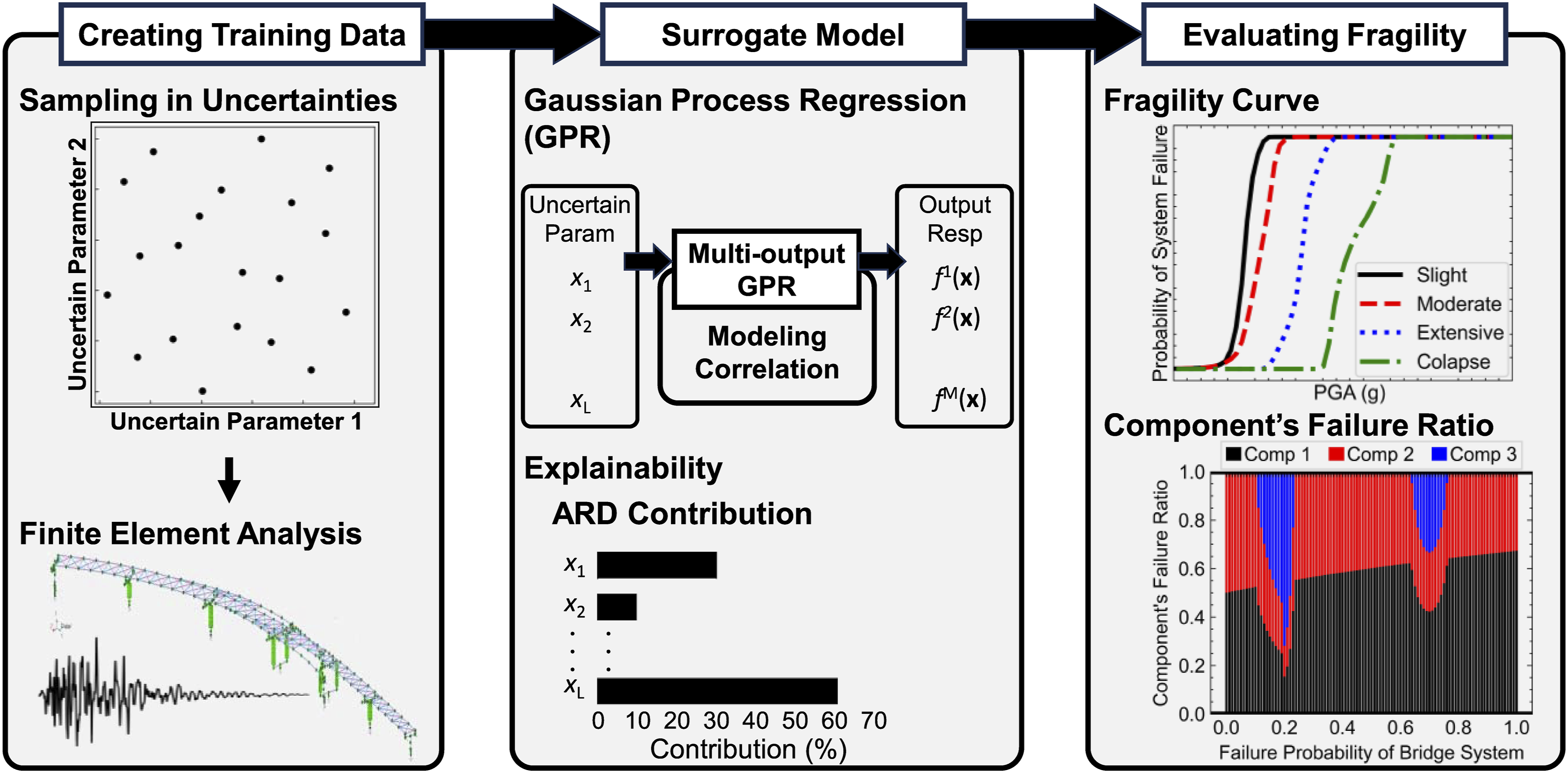

This section first presents the formulation of the multi-output GPR and explains the ARD kernel and derivation of the contribution of each input-parameter uncertainty to the output from the estimated hyperparameter. Subsequently, a general formulation of the fragility curve and its derivation using the constructed surrogate model are presented. In addition, the methodology of the statistical failure-mode evaluation in the system failure is presented.

Multi-output Gaussian process regression

GPR is a nonparametric regression model that can provide predictive variance and is generally recognized as robust to overlearning. The typical GPR cannot model the correlations among outputs. However, many cases require multiple outputs, and a correlation between the demand outputs in some modeling targets, including the structural responses under loadings, may be assumed. Therefore, this study adopts the multi-output GPR developed by Bonilla et al. (2007).

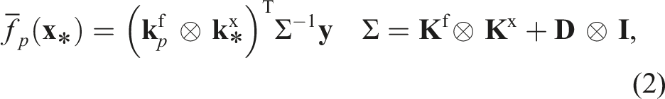
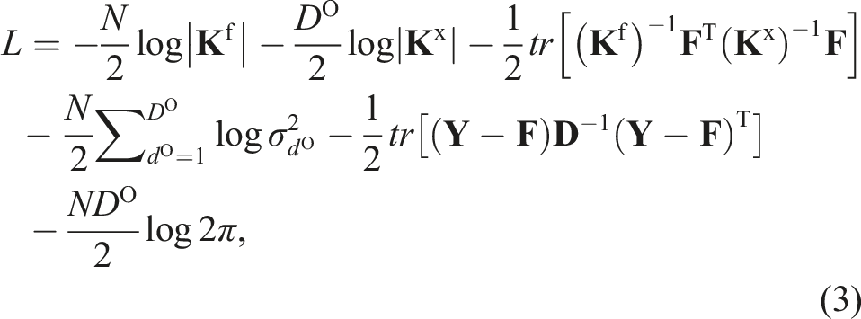
In the formulation of the multi-output GPR used in this study, the assumed numbers of input and output parameters of the GPR model are $D^{I}$ and $D^{O}$ , respectively. The input vectors of the training data of size N are $x_{1}, x_{2}, \dots, x_{N}$ , where the length of $x_{i}$ $(i = 1 - N)$ is $D^{I}$ . The output vector is then configured as $y = {(y_{11}, \dots, y_{N 1}, \dots, y_{12}, \dots, y_{N 2}, \dots, y_{1 D^{O}}, \dots, y_{N D^{O}})}^{T}$ for the $D^{O}$ outputs in each training dataset. To induce correlations among the outputs, the prior Gaussian process is assumed for the latent functions $f_{p}$ and $f_{o}$ as follows:

f_{p} (x) f_{o} (x^{'}) = K_{p o}^{f} k (x, x^{'}) y_{i p} \sim N (f_{p} (x_{i}), σ_{p}^{2}),

(1)

where

K_{p o}^{f}

is the element in row

p (p = 1 - D^{O})

and column

o (o = 1 - D^{O})

of the constant-value matrix.

K_{p o}^{f}

determines the similarity between the outputs, k is the kernel function for the input, and

σ_{p}

represents the noise for the pth output dimension. The correlations among the

D^{O}

outputs are represented by

K_{p o}^{f}

. For the predictions made by this model, the mean and variance can be obtained by the kernel function k in equation (1), which is the same procedure used in the typical GPR. For example, the mean prediction for the new input data

x_{*}

in the output dimension p can be expressed as:

{\bar{f}}_{p} (x_{*}) = {(k_{p}^{f} \otimes k_{*}^{x})}^{T} Σ^{- 1} y Σ = K^{f} \otimes K^{x} + D \otimes I,

(2)

where

\otimes

is the Kronecker product and

k_{p}^{f}

is pth column of

K^{f}

k_{*}^{x}

is the covariance vector of

x_{*}

and the training data

x_{i}

K^{x}

is a covariance matrix over all training data, and D is a diagonal matrix with a size of

D^{O} \times D^{O}

, where its (k, k)-th element is

σ_{k}^{2}

. In addition, the GPR optimization involves maximizing the log-likelihood, represented as follows:

\begin{array}{l} L = - \frac{N}{2} \log | K^{f} | - \frac{D^{O}}{2} \log | K^{x} | - \frac{1}{2} t r [{(K^{f})}^{- 1} F^{T} {(K^{x})}^{- 1} F] \\ - \frac{N}{2} \sum_{d^{O} = 1}^{D^{O}} \log σ_{d^{O}}^{2} - \frac{1}{2} t r [(Y - F) D^{- 1} {(Y - F)}^{T}] - \frac{N D^{O}}{2} \log 2 π \end{array},

(3)

where Y is an

N \times D^{O}

matrix consisting of the outputs of the training data and F is the matrix of function values corresponding to Y. In this study, the adaptive moment (Adam) optimizer (Kingma and Ba, 2014) was used to maximize equation (3) during the training process and a GPR model was constructed using the Python library GPyTorch (Gardner et al., 2018).

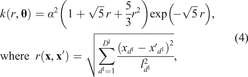
ARD kernel in GPR and estimation of contributions to outputs

To improve the explanatory power of surrogate modeling, knowing which and to what extent the uncertain parameters contribute to the output is important. Knowing the parameter contributions during the training of the GPR model allows to determine whether they are valid from an engineering standpoint, and the validity of the surrogate model can be discussed. For GPR, the ARD kernel was adopted to quantify the contribution of each $D^{I}$ input parameter by employingthe Matern5/2 kernel function with the ARD kernel for the kernel function k in equation (1), which can be expressed as follows:

k (r, θ) = α^{2} (1 + \sqrt{5} r + \frac{5}{3} r^{2}) \exp (- \sqrt{5} r), where r (x, x^{'}) = \sqrt{\sum_{d^{I} = 1}^{D^{I}} \frac{{(x_{d^{I}} - {x^{'}}_{d^{I}})}^{2}}{l_{d^{I}}^{2}}},

(4)

where

θ

is a vector of the hyperparameters

α

and

l_{d^{I}} (d^{I} = 1 - D^{I})

l_{d^{I}}

is the length scale that represents the contribution of the

d^{I}

-th input parameter to the outputs. The smaller the length scale, the larger the value of the kernel function k, indicating a greater contribution. These hyperparameters, including

l_{d^{I}}

, are also estimated by maximizing equation (3), implying that the contributions are estimated automatically. Based on the estimated length scale

l_{d^{I}}

, the normalized contribution

c_{d^{I}}

is derived as a percentage, as follows:

c_{d^{I}} = \frac{1 / l_{d^{I}}}{\sum_{k = 1}^{D^{I}} (1 / l_{k})} \times 100 (d^{I} = 1, 2, . . ., D^{I}) .

(5)

This contribution $c_{d^{I}}$ indicates the relative contribution within the input parameters to outputs.

Calculating fragility curve and estimating component contributing to system fragility

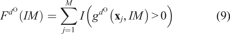
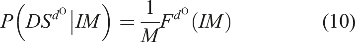
Fragility curves represent the conditional probability, that is, the probability that the structure fails above a particular damage level for a given seismic intensity (Billah and Alam, 2015; Mackie and Stojadinović, 2005). The probability of failure P of the $d^{O}$ -th structural member is formulated as follows:

P (D S^{d^{O}} | I M) = P (D^{d^{O}} > C^{d^{O}} | I M),

(6)

where IM is the intensity measurement of the earthquake, DS is the damaged state, D is the demand response to be evaluated for the structural members, and C is the capacity level of the structural member. In other words, equation (6) represents the probability that the demand response exceeds the capacity level at a given seismic-intensity measure, IM. Suppose the performance function

Z = D - C

P (D S^{d^{O}} | I M) = P (Z^{d^{O}} > 0 | I M) .

(7)

The variable of function Z depends on the uncertainties of the structural parameters or intensity measures, and these parameters become the input in the multi-output GPR surrogate model x. Thus, Z can be expressed as a function g of x and IM as follows:

P (D S^{d^{O}} | I M) = P (g^{d^{O}} (x, I M) > 0) .

(8)

Generally, the least-squares-based approach, which assumes that D and C follow a log-normal distribution, and the maximum-likelihood estimation-based approach, which assumes lognormality of the fragility curve, are used to obtain this probability; however, the errors are large when deviating from that assumption. Therefore, in this study, function $g^{d^{O}}$ in equation (8) is modeled by the multi-output GPR surrogate model. Using the constructed surrogate model, the probability in equation (8) is obtained by Monte Carlo calculation as follows:

F^{d^{O}} (I M) = \sum_{j = 1}^{M} I (g^{d^{O}} (x_{j}, I M) > 0)

(9)

P (D S^{d^{O}} | I M) = \frac{1}{M} F^{d^{O}} (I M)

(10)

where M is the number of samples in the Monte Carlo calculation and I is a function that returns a value of one when the condition in parentheses is satisfied, and zero otherwise.

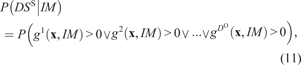
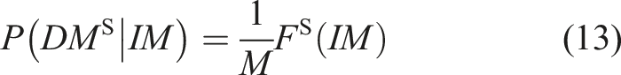
The system fragility is also derived from the MC calculation using a surrogate model. Assuming that bridge system S is defined as a series system, that is, at least one of the components reaches or exceeds its limit states, the joint probability is represented as,

P (D S^{S} | I M) = P (g^{1} (x, I M) > 0 \lor g^{2} (x, I M) > 0 \lor . . . \lor g^{D^{O}} (x, I M) > 0),

(11)

where

D^{O}

is the number of structural components related to system failures. As considered in equation (9), the failure probability of the system

F^{S}

is calculated using the surrogate model as follows:

F^{S} (I M) = \sum_{j = 1}^{M} I (g^{1} (x_{j}, I M) > 0 \lor g^{2} (x_{j}, I M) > 0 \lor . . . \lor g^{D^{O}} (x_{j}, I M) > 0)

(12)

P (D M^{S} | I M) = \frac{1}{M} F^{S} (I M)

(13)

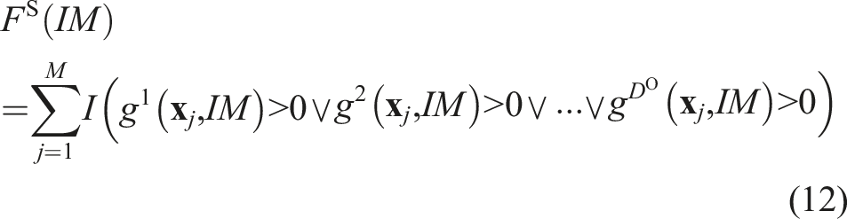
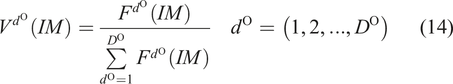
Furthermore, this study identifies component failures that statistically contribute to system failures. The failure ratio $V^{d^{O}}$ is an index for evaluating the contribution of the $d^{O}$ -th component, which is calculated as follows:

V^{d^{O}} (I M) = \frac{F^{d^{O}} (I M)}{\sum_{d^{O} = 1}^{D^{O}} F^{d^{O}} (I M)} d^{O} = (1, 2, . . ., D^{O})

(14)

where

F^{d^{O}}

is the counted number of failure events derived in equation (9). The higher this value, the more the

d^{O}

-th structural component contributed to the system failure.

Equations (11)–(13) show the derivation of the system fragility for a particular limit state associated with system failure owing to the series assumption. The verification of the system fragility of a bridge system in Section 3.3 also uses the same definition. However, the GPR surrogate model can perform fragility analyses with any definition of system failure.

Seismic fragility evaluation of seismic isolation highway bridge

The multi-output GPR surrogate model in this study was verified by applying it to the fragility analysis of a seismic isolation highway bridge. Because this is an actual bridge, its detailed structural properties and seismic-design documentation were shared by the bridge owner. In this section, the FE-model construction of the bridge and nonlinear seismic-response analysis are first presented. The uncertainties of the parameters to be considered and the demand responses for the fragility analysis are recognized to determine the inputs and outputs of the surrogate model. Finally, the limit states of the structural failures are determined at both the component and system levels.

FE modeling for seismic-response analysis

The target highway bridge is a seismic isolation six-span continuous two-steel box-girder bridge with a curved geometry, a total length of 327.9 m, and a width of 13–16.95 m. The bridge is located on ground with soil type 2, which is defined as hard ground. The substructure of the bridge consists of five steel piers, one concrete pier, and abutments. Some of the piers are gate-shaped and located where the merging lane converges with the main line. The sub- and super-structure are isolated by employing a total of 22 seismic isolation bearings at the top of piers and abutment.

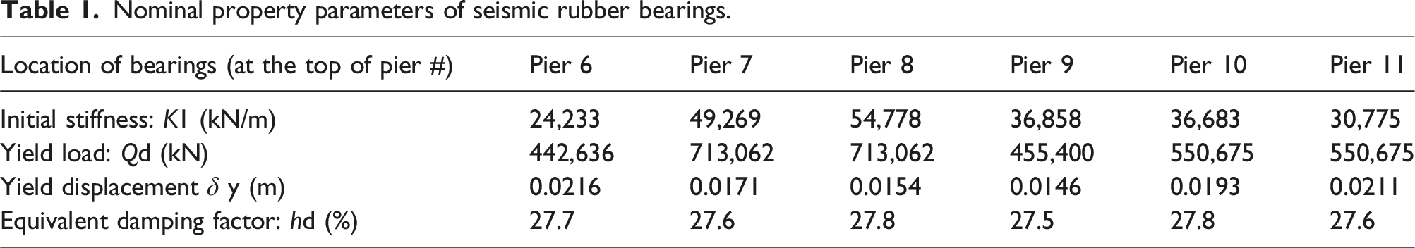
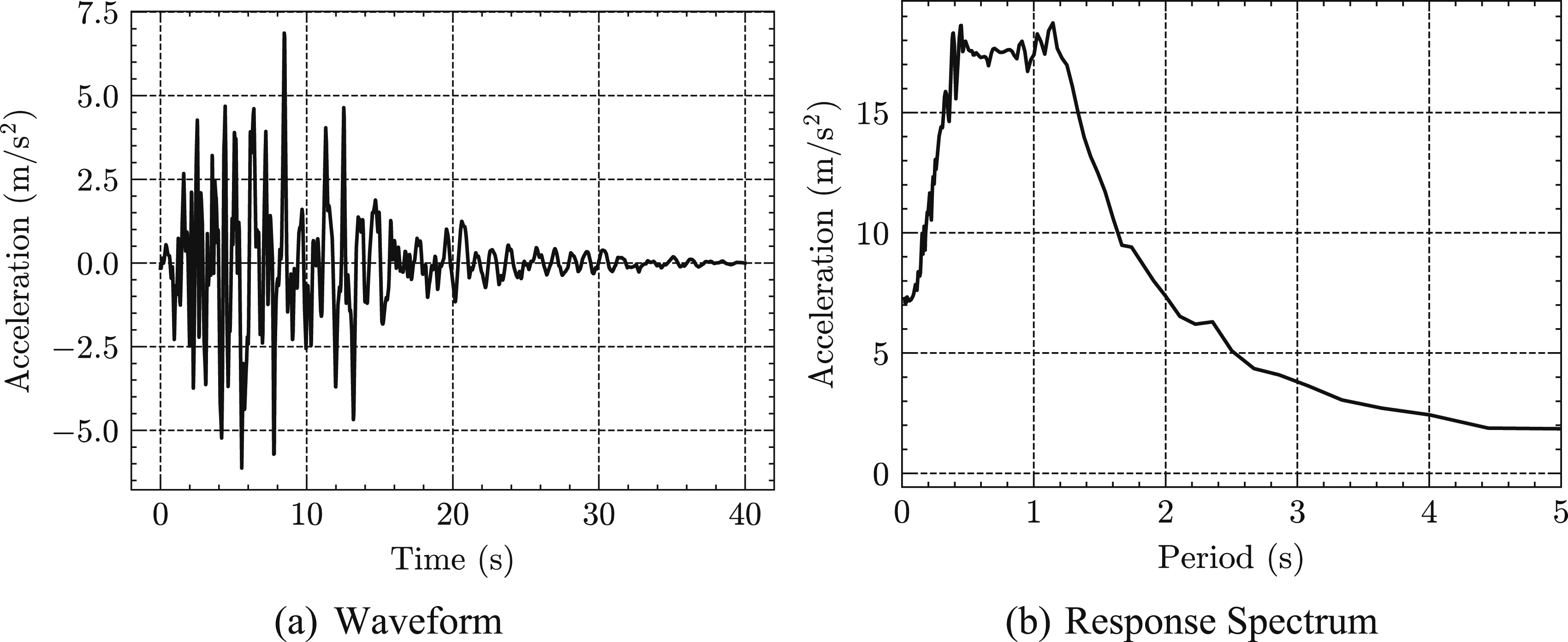
A three-dimensional FE model of the bridge was constructed for our study (Rashid and Nishio, 2023) according to the properties described in the design drawings and design documentation. The modeling and numerical calculations were implemented using software for the bridge FE-model analysis: Engineer’s Studio (FORUM8, 2019). Figure 2 shows an overview of the constructed frame FE model of the bridge and material constitutive models for the rubber bearings, steel, and concrete piers.. Seismic rubber bearings are represented by multi-shear spring elements that ensure consistent nonlinear characteristics throughout the horizontal plane (Wada and Hirose, 1989). The nonlinear property is described by a bilinear model, where the secondary stiffness K2 after yielding is fixed at 15% of the initial stiffness K1. Table 1 summarizes the parameters of the bilinear model for the rubber bearings on each pier, which were determined and introduced in the design documentation. The superstructure was represented by linear beam elements that remains elastic under dynamic loading. The steel piers, partially filled with concrete, were modeled as fiber elements, representing nonlinear stress-strain steel and concrete properties. For the steel-material nonlinearity, the bilinear stress-strain relationship was adopted with a strain hardening of 1% of the Young’s modulus. The properties of these steel members were determined based on the adopted steel types: SM490 and SS400. The properties of the reinforced concrete pier were determined based on the material properties of the concrete with compressive strength and those of the steel bar, which are also shown in the design documentation. Considering the anticipated plasticity near the base of the concrete piers (plastic hinge zone), nonlinearities were incorporated using the nonlinear Takeda model (Takeda et al., 1970). Boundary conditions were provided to represent the interaction between the substructure and soil by six linear springs (three translational and three rotational) at each pier’s base, whose properties were also consistent with the values in the design documentation. The dynamic seismic response was calculated by the nonlinear time-history analysis with the input waveform of one of the design loads: “Level2 Type2-2-1,” introduced in the Japanese design standard (Japan Road Association, 2016). This design seismic load was set based on the record of the 1995 Kobe Earthquake at the Japan Railway Takatori Station. The waveform and response spectra derived for the acceleration with a damping ratio of 5% are shown in Figure 3. In the numerical calculation, the time increment for numerical integration was fixed to 0.01 s, confirming that no divergence occurred.

Figure 2.

Finite-element model of bridge system.

Table 1.

Nominal property parameters of seismic rubber bearings.

Location of bearings (at the top of pier #)	Pier 6	Pier 7	Pier 8	Pier 9	Pier 10	Pier 11
Initial stiffness: K1 (kN/m)	24,233	49,269	54,778	36,858	36,683	30,775
Yield load: Qd (kN)	442,636	713,062	713,062	455,400	550,675	550,675
Yield displacement δ y (m)	0.0216	0.0171	0.0154	0.0146	0.0193	0.0211
Equivalent damping factor: hd (%)	27.7	27.6	27.8	27.5	27.8	27.6

Figure 3.

Input seismic load (Level 2 Type 2-2-1 seismic design load). (a) Waveform (b) Response Spectrum.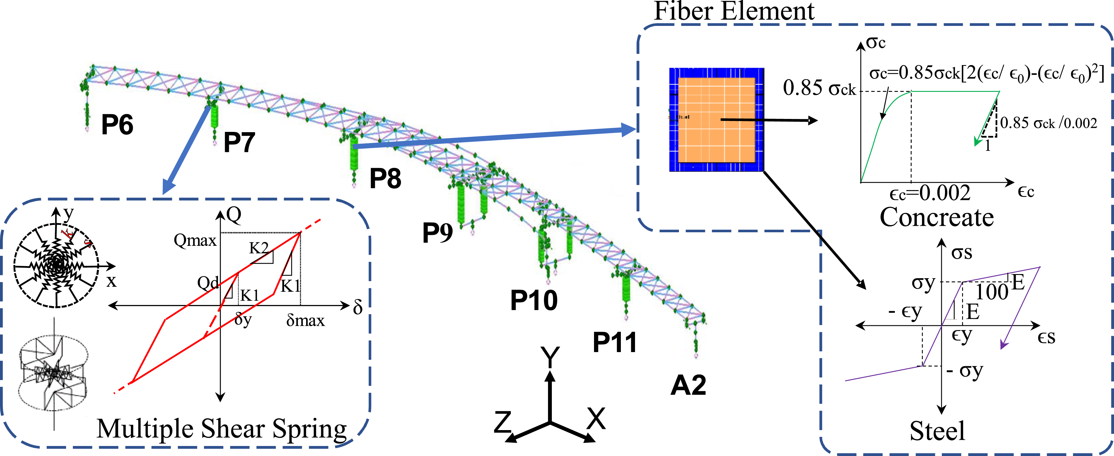

The validity of the FE model was verified by confirming that the calculated resonant modes and time-history responses were consistent with those under the same input seismic waveform shown in the design documentation. Table 2 shows the resonant frequencies/periods and effective masses of the first 10 modes, whose periods are in the dominant range of approximately 0.4−1.3 s in the response spectra of the seismic waveform shown in Figure 3(b). The bridge has the characteristics of resonant modes with significant effective masses in Modes 1, 2, 8, and 10. The shapes of the modes are shown in Figure 4. Large modal displacements occurred at the steel piers, from P8 to P11, and the abutment in Mode 1, whereas concrete pier P6 showed particularly large displacements in Modes 2, 8, and 10.

Table 2.

Resonant mode characteristics of seismic isolation highway bridge.

Mode #	Frequency (Hz)	Period (s)	Effective mass (t)
Mode #	Frequency (Hz)	Period (s)	X	Y	Z
Mode 1	0.630	1.587	1.793	0.016	4340.920
Mode 2	0.664	1.506	4930.203	0.054	0.055
Mode 3	0.694	1.441	55.264	0.057	122.833
Mode 4	0.833	1.200	0.700	0.049	160.746
Mode 5	1.158	0.864	1.485	0.049	94.079
Mode 6	1.209	0.827	7.575	0.029	88.114
Mode 7	1.450	0.690	5.305	5.005	13.495
Mode 8	1.673	0.598	1317.255	3.250	91.808
Mode 9	1.718	0.582	0.117	129.920	65.515
Mode 10	1.777	0.563	49.449	21.327	947.398

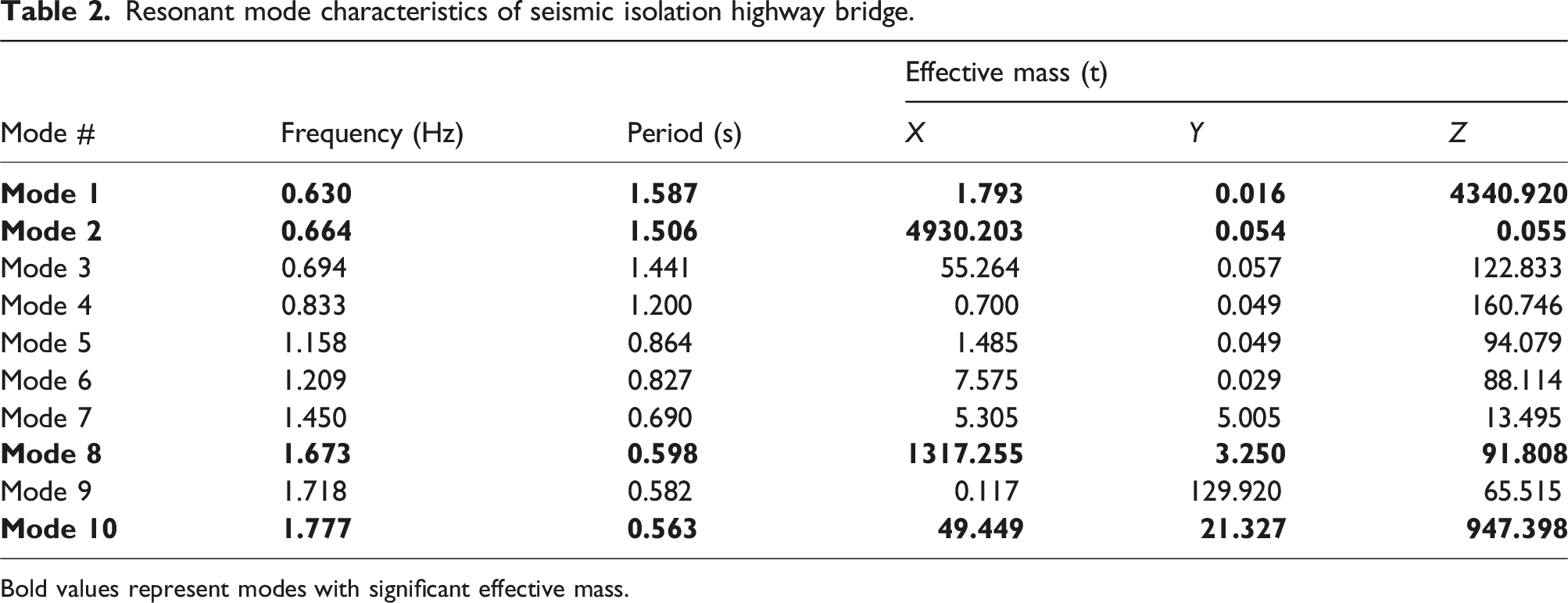
Bold values represent modes with significant effective mass.

Figure 4.

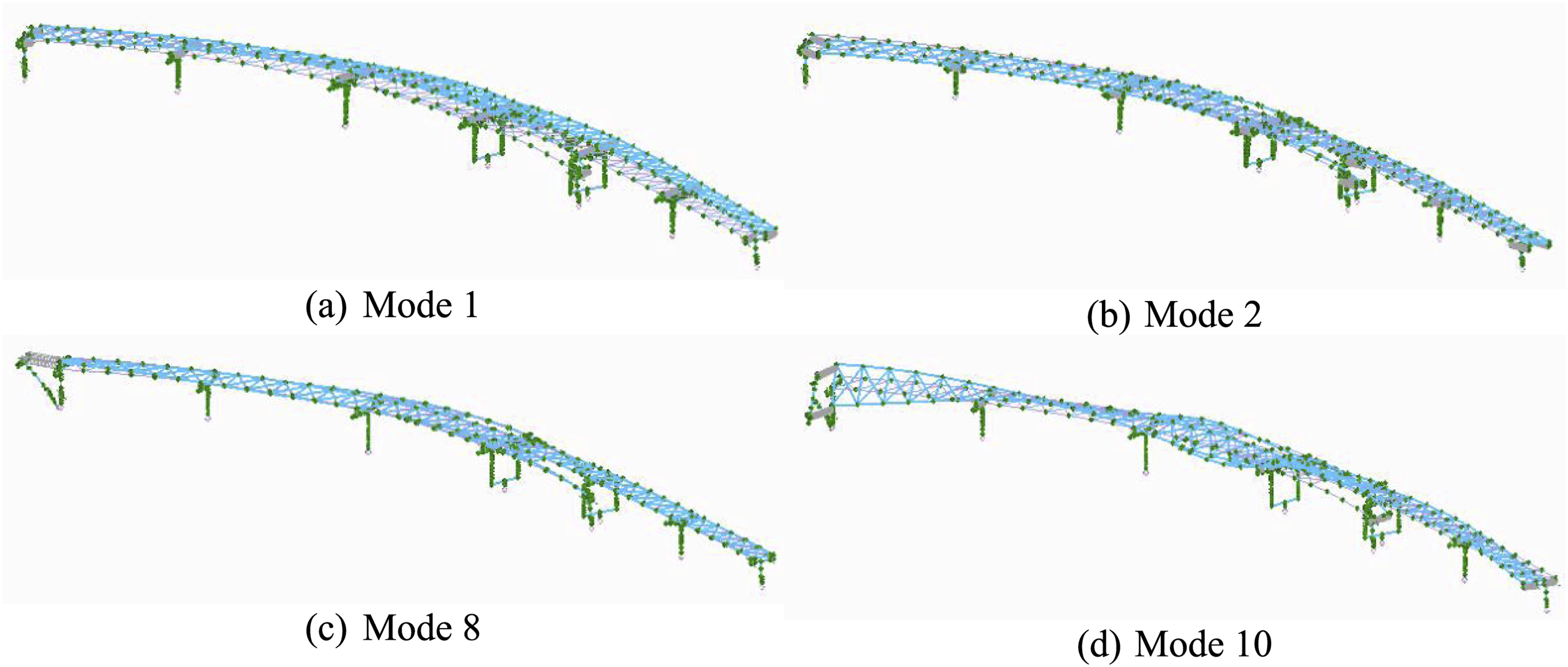
Modal shapes of seismic isolation highway bridge. (a) Mode 1 (b) Mode 2 (c) Mode 8 (d) Mode 10.

Uncertainties considered in fragility analysis and inputs-outputs of surrogate model

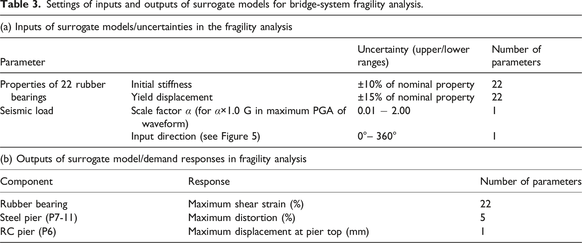
In general, all possible uncertainties should be considered when conducting the uncertainty analysis, such as fragility or risk analysis. The uncertainties of the considered parameters represented by probability distributions should be determined based on the requirements and policy of the fragility/risk analysis, including which uncertainties and how these uncertainties should be considered. These uncertain parameters are included as input variables for the surrogate model. Additionally, the parameter variables in the fragility analysis, such as the intensity measure of the seismic load, are included in the input variables of the surrogate model. The outputs of the surrogate model are the demand responses used to evaluate whether they exceed the defined limit states for calculating the failure probability. The multi-output GPR surrogate model can simultaneously result in multiple output demand responses.

Table 3 (a) and (b) present the 46 inputs and 28 outputs of the surrogate model for the fragility analysis of the bridge system in this study, respectively. For the inputs, the properties of all 22 rubber bearings installed in the target highway bridge are set as uncertain parameters for the structural properties, because the dominant structural member that contributes to the seismic performance of a seismic isolation bridge is the seismic rubber bearing. Each rubber bearing has two properties, initial stiffness K1 and yield displacement δ _Y, because the secondary stiffness of the bilinear model is determined to be approximately 15% of the initial stiffness, as mentioned in the previous section. The ranges of these two parameters are set to ±10% and ±15% of their nominal properties, respectively, which are determined based on previous studies or surveys of variations in rubber-bearing properties. Note that the 44 uncertain parameters are considered independent variables. For the uncertainties in the seismic load, the Level 2 type 2-2-1 waveform is applied at varying input excitation direction, ranging from 0° to 360° in the horizontal plane, as shown in Figure 5. The uncertainty of the input seismic direction may significantly affect the failure mode and probability, particularly when considering the system fragility in the target bridge with a curved geometry. A single seismic waveform is acceptable in the fragility analysis for evaluating whether the target bridge satisfies the capacities originally required in the design phase. Therefore, the fragility analysis in this study is adopted to consider the uncertainties of the input directions by fixing the seismic waveform. To derive the fragility curves, the intensity measure of the seismic load must be changed; thus, a relevant parameter is included in the input variables of the surrogate model. A scaling coefficient α is introduced to scale the fixed waveform from 0.01 g to 2.00 g as the maximum PGA, where the range is determined based on recent related studies (Montazeri et al., 2021; Thapa et al., 2022).

Table 3.

Settings of inputs and outputs of surrogate models for bridge-system fragility analysis.

(a) Inputs of surrogate models/uncertainties in the fragility analysis
Parameter		Uncertainty (upper/lower ranges)	Number of parameters
Properties of 22 rubber bearings	Initial stiffness	±10% of nominal property	22
Properties of 22 rubber bearings	Yield displacement	±15% of nominal property	22
Seismic load	Scale factor α (for α×1.0 G in maximum PGA of waveform)	0.01 − 2.00	1
Seismic load	Input direction (see Figure 5)	0°– 360°	1

(b) Outputs of surrogate model/demand responses in fragility analysis
Component	Response	Number of parameters
Rubber bearing	Maximum shear strain (%)	22
Steel pier (P7-11)	Maximum distortion (%)	5
RC pier (P6)	Maximum displacement at pier top (mm)	1

Figure 5.

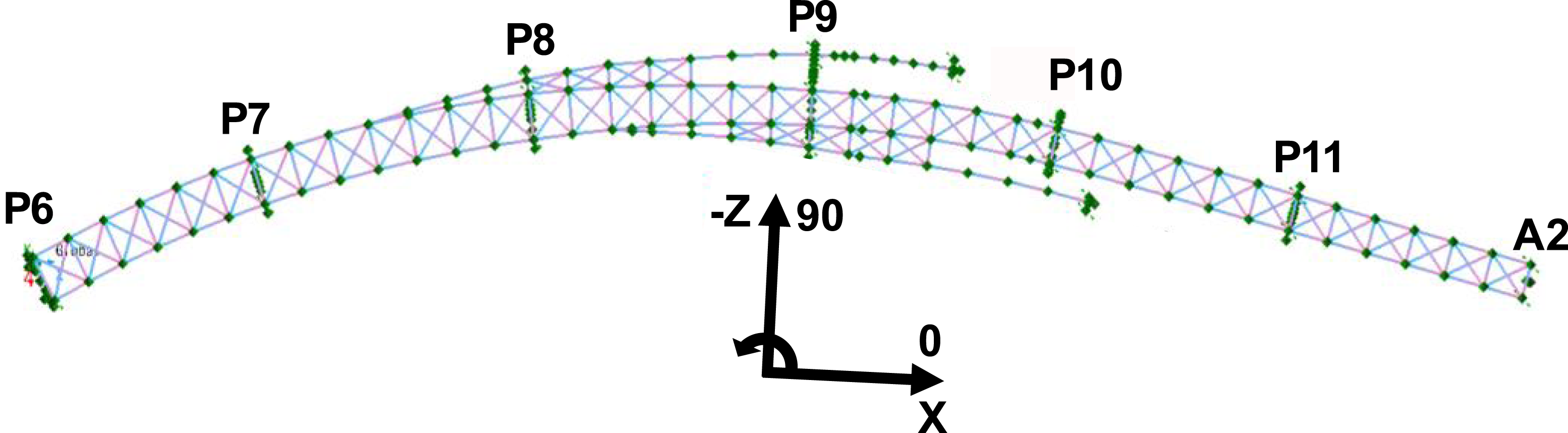
Definition of input direction of seismic load.

In this study, the fragility analysis considered the uncertainties of the input directions and intensities against the design waveform (Japan Road Association, 2016). This type of evaluation is also significant in the performance analysis of target structures in demand for the retrofitting or maintenance of existing structures.

The outputs of the surrogate model are consistent with the demand responses that exceed the defined limit states. The maximum shear strain of each rubber bearing, maximum distortion at each steel pier, and maximum horizontal displacement at the top of the concrete pier are evaluated; thus, the number of outputs of the surrogate model is 28, as shown in Table 3 (b). The definitions of the limit states at the component and system levels are presented in the next section.

The training data for constructing the surrogate model are created by conducting FE analyses using the generated samples of input-parameter vectors from the 46-dimensional parameter space of the uniform distributions. A uniform distribution realizes samples with even probabilities across the entire possible range of the parameter space. The surrogate model, developed using the training data of input variables with uniform distributions, realizes a fragility analysis considering any probability distribution of the input parameter. However, in this study, the same uniform distributions with lower and upper bounds shown in Table 3 (a) are adopted for the uncertainties considered in the fragility analysis of the highway bridge system.

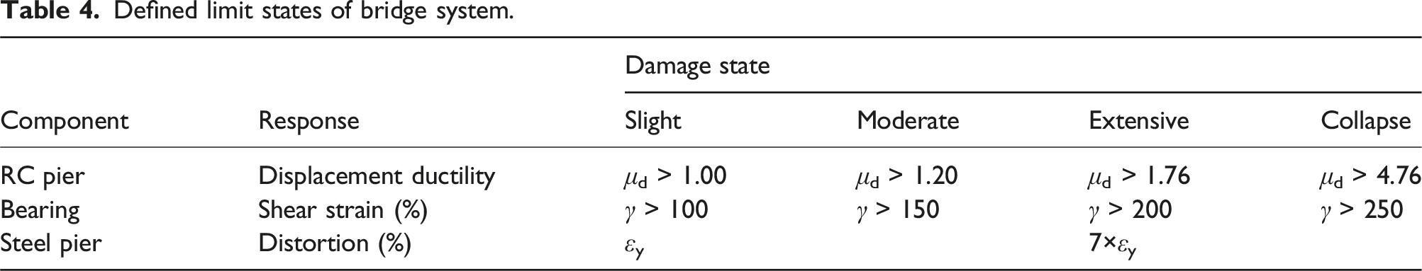
Limit-state definitions for bridge components and system

In continuous bridge systems incorporating seismic isolation bearings, the isolation bearings and piers have emerged as pivotal components that frequently exhibit nonlinear behavior during seismic events. Hence, seismic isolation bearings, RC piers, and steel piers are considered critical constituents, and limit states are established. The evaluation of these limit states encompasses the utilization of shear strain for bearings, displacement ductility for RC piers, and distortion for steel piers. The performance assessment adheres to the qualitative damage criteria of the HAZUS model developed by Federal Emergency Management Agency(Hazus, 2021) and delineates four distinct damage states: Slight, Moderate, Extensive, and Collapse. Table 4 lists the settings of the limit state of the bridge system. The limit state of RC pier is described by the displacement ductility ratio, that is, the displacement relative to the initial yield displacement, drawn from previous studies. The determination of the limit state for bearings is based on empirical observations and impactconsideration of secondary damage progression, including pounding effects at abutments. In the context of the bridges considered in this study, the limit states are ascertained through the dimensionless shear strain, accounting for the variabilities in the dimensions of the bearings. For steel piers, the definition of limit states is grounded in the design documents. Minor damage states refer to the onset of reaching the yield strain, whereas severe damage states are quantified based on the ultimate strain.

Table 4.

Defined limit states of bridge system.

Component	Response	Damage state
Component	Response	Slight	Moderate	Extensive	Collapse
RC pier	Displacement ductility	μ_d > 1.00	μ_d > 1.20	μ_d > 1.76	μ_d > 4.76
Bearing	Shear strain (%)	γ > 100	γ > 150	γ > 200	γ > 250
Steel pier	Distortion (%)	ε _y		7×ε_y

Results of surrogate modeling for seismic fragility analysis

In this section, a fragility analysis of the bridge system described in Section 3 is performed using the surrogate model with the multi-output GPR model described in Section 2. First, the multi-output GPR model is compared with the GPR model with independent outputs to verify the effectiveness of modeling the correlation of the outputs. The accuracy of the surrogate model is calculated using the coefficient of determination to ascertain the amount of training data required for sufficiently accurate GPR surrogate modeling. Next, we discuss the explainability of the surrogate model in terms of the contribution of each uncertain parameter to the output obtained based on the length scale of the ARD kernel. A fragility curve is calculated using the GPR surrogate model, which has accuracy and explainability. Subsequently, the effect of the seismic input angle on the fragility curve is discussed. Finally, a GPR surrogate model is used to estimate the structural components that contribute to the failure of the bridge system.

Accuracy of multi-output GPR surrogate model

To verify the surrogate-model construction, 500 input–output data points are first created by FE analysis using 500 input parameter sets sampled by the Latin Hypercube Sampling method (LHS) from the 46-dimensional space of input variables. To compare the performances of the constructed surrogate models by varying the amount of training datapoints N, N datapoints are randomly sampled for training from the base dataset configured from the 500 datapoints, and the remaining 500-N datapoints are used as the test dataset. LHS allows for sparse sampling by ensuring that no duplicate rows occur during the grid division. Even the random sampling of N samples from the 500 samples, which were created by LHS, exhibit the same stochastic process. Thus, the dataset in each case of the N training datapoints can adequately represent the same parameter space. Using N inputs and multiple outputs created by the FE analysis, the multi-output GPR surrogate model is obtained by applying the procedures presented in Sections 2.1 and 2.2.

The accuracy of the constructed surrogate model using n training datapoints, where n is the variable of the number of training datapoints N, is evaluated using the coefficient of determination R² for the test dataset, which is configured using 500-N datapoints, as described in: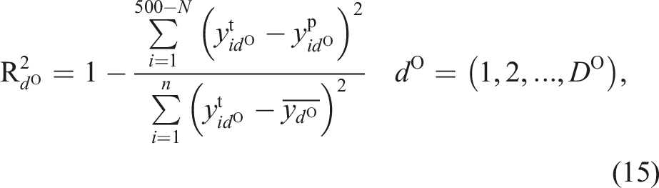

R_{d^{O}}^{2} = 1 - \frac{\sum_{i = 1}^{500 - N} {(y_{i d^{O}}^{t} - y_{i d^{O}}^{p})}^{2}}{\sum_{i = 1}^{n} {(y_{i d^{O}}^{t} - \bar{y_{d^{O}}})}^{2}} d^{O} = (1, 2, . . ., D^{O}),

(15)

where

y_{i d^{O}}^{t}

is the true value of the demand responses listed in Figure 3(b) obtained by the FE analysis for ith datapoint of the test dataset, and

y_{i d^{O}}^{p}

is the predicted demand response of the surrogate model assigning the ith data input.

\bar{y_{d^{O}}}

represents the mean value of the demand responses within the test dataset. The R² statistic approaches one as the prediction becomes more accurate, and is commonly used in accuracy evaluations of machine-learning models. To verify the influence of the amount of training data on the accuracy of the surrogate model, N is evaluated from 25 to 300 in 25 data intervals. In each case, random sampling of the training data from the base dataset of 500 datapoints is repeated 10 times, and the mean and standard deviation (std) of the R² statistics for 10 surrogate models are derived to verify the accuracy and stability of the surrogate model.

Figure 6 shows variation of R² averaged over the total output-dimension statistics with the mean and std increasing the number of training datapoints. The solid line represents the mean value, and the ranges indicate the upper and lower bounds of the std. The red line is the result of the multi-output GPR model, and the blue line is the result of the typical GPR model with a single output. The R² statistics of the multi-output GPR models show higher values than those of GPR models with a single output for any number of training datapoints in the range examined, which indicates that the multi-output GPR model can provide accurate surrogate models. The stability of prediction in the multi-output GPR model is also higher than that of the GPR model with a single output because the std quickly converges to smaller ranges. The accuracy of the multi-output GPR model reaches approximately 0.98 in R² value with 75 training datapoints, and the same accuracy is achieved with approximately 125 training datapoints in the GPR model with a single output. This means that sufficient accuracy can be achieved with 40% fewer training datapoints compared to the GPR model with a single output. The achievements of high accuracy and stability in the multi-output GPR model can be explained. The model can represent correlations within the multiple outputs, for example, the correlation between maximum shear strains of rubber bearings on the neighboring piers. This result emphasizes the importance of modeling the correlations of outputs when the responses of several components are required as outputs of the surrogate model.

Figure 6.

Accuracy and stability of GPR surrogate models increasing with number of training datapoints.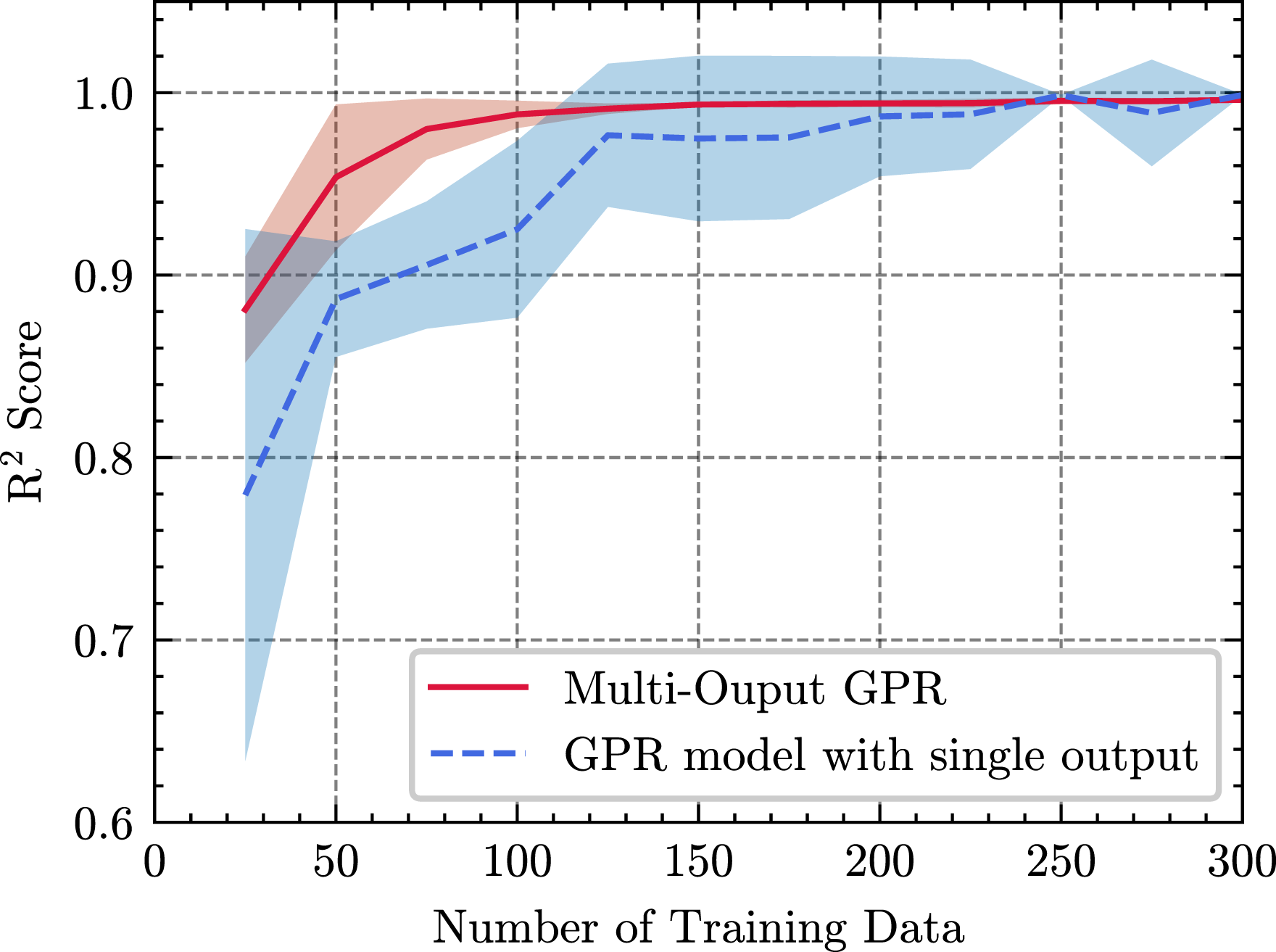

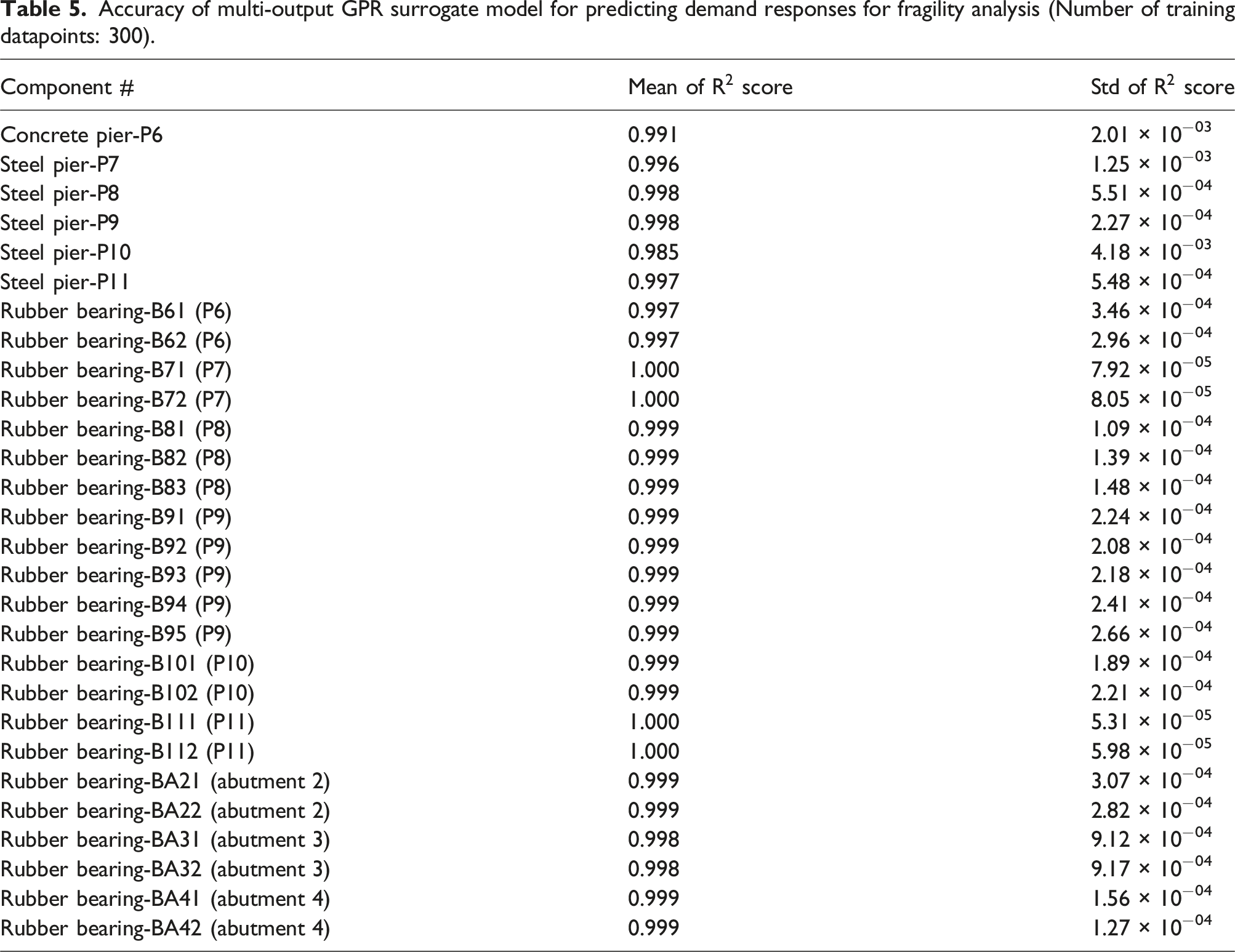
Although the accuracy and stability are sufficient for the model to converge with 150 training datapoints in the multi-output GPR surrogate model, the model constructed using 300 training datapoints is used in the verification of the fragility analysis in the next section for confident verifications. Table 5 summarizes the R² values for the 28 demand responses in the case of 300 training datapoints. For all demand responses, R² values are 0.98 or higher with sufficiently low variations.

Table 5.

Accuracy of multi-output GPR surrogate model for predicting demand responses for fragility analysis (Number of training datapoints: 300).

Component #	Mean of $R^{2}$ score	Std of $R^{2}$ score
Concrete pier-P6	0.991	2.01 × 10⁻⁰³
Steel pier-P7	0.996	1.25 × 10⁻⁰³
Steel pier-P8	0.998	5.51 × 10⁻⁰⁴
Steel pier-P9	0.998	2.27 × 10⁻⁰⁴
Steel pier-P10	0.985	4.18 × 10⁻⁰³
Steel pier-P11	0.997	5.48 × 10⁻⁰⁴
Rubber bearing-B61 (P6)	0.997	3.46 × 10⁻⁰⁴
Rubber bearing-B62 (P6)	0.997	2.96 × 10⁻⁰⁴
Rubber bearing-B71 (P7)	1.000	7.92 × 10⁻⁰⁵
Rubber bearing-B72 (P7)	1.000	8.05 × 10⁻⁰⁵
Rubber bearing-B81 (P8)	0.999	1.09 × 10⁻⁰⁴
Rubber bearing-B82 (P8)	0.999	1.39 × 10⁻⁰⁴
Rubber bearing-B83 (P8)	0.999	1.48 × 10⁻⁰⁴
Rubber bearing-B91 (P9)	0.999	2.24 × 10⁻⁰⁴
Rubber bearing-B92 (P9)	0.999	2.08 × 10⁻⁰⁴
Rubber bearing-B93 (P9)	0.999	2.18 × 10⁻⁰⁴
Rubber bearing-B94 (P9)	0.999	2.41 × 10⁻⁰⁴
Rubber bearing-B95 (P9)	0.999	2.66 × 10⁻⁰⁴
Rubber bearing-B101 (P10)	0.999	1.89 × 10⁻⁰⁴
Rubber bearing-B102 (P10)	0.999	2.21 × 10⁻⁰⁴
Rubber bearing-B111 (P11)	1.000	5.31 × 10⁻⁰⁵
Rubber bearing-B112 (P11)	1.000	5.98 × 10⁻⁰⁵
Rubber bearing-BA21 (abutment 2)	0.999	3.07 × 10⁻⁰⁴
Rubber bearing-BA22 (abutment 2)	0.999	2.82 × 10⁻⁰⁴
Rubber bearing-BA31 (abutment 3)	0.998	9.12 × 10⁻⁰⁴
Rubber bearing-BA32 (abutment 3)	0.998	9.17 × 10⁻⁰⁴
Rubber bearing-BA41 (abutment 4)	0.999	1.56 × 10⁻⁰⁴
Rubber bearing-BA42 (abutment 4)	0.999	1.27 × 10⁻⁰⁴

Explainability of constructed multi-output GPR surrogate model

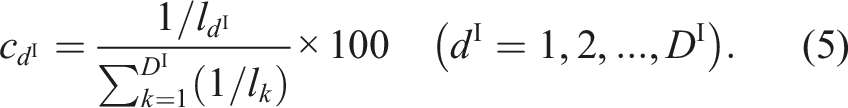
The contribution of these uncertainty parameter results from the length scale of the ARD kernel of the GPR, which is computed using equation (5). From the characteristic length scale of the ARD kernel, the contribution (the sensitivity), of the uncertain parameters to the output response can be calculated. By observing these contributions, the parameters affecting the output response can be understood, thereby enhancing the explainability of the surrogate models. As described in Section 4.1, a surrogate model is constructed in this verification by increasing the training datapoints by 25, from 25 to 300. The surrogate model is constructed 10 times for each training dataset.

Figure 7 shows the convergence of the rate of change of the contribution of the uncertain parameters derived by the estimated ARD based on the number of training datapoints. The vertical axis is the rate of change of the contributions from the current number of datapoints to that one step before. For example, the value at 50 training datapoints is the ratio of the difference in contributions between 50 and 25 training datapoints to the contribution at 25 training datapoints. The solid line represents the mean for all uncertain parameters over 10 trials, and the range shows the std. With the increase in training data points , the contribution rate change estimated from the ARD kernel tends to decrease. In particular, when the number of training datapoints exceeds 200, the average of the contribution change rate is less than 5%, indicating that the contribution does not change significantly. Figure 7 shows that the accuracy of the GPR surrogate model remains largely the same after 200 training datapoints. This suggests that the accuracy convergence of the GPR surrogate model can be understood by examining the changes in the contribution values of the ARD kernel uncertainty parameters. In other words, the accuracy convergence of the GPR surrogate model can be ascertained even in the absence of test data.

Figure 7.

Convergence of contributions estimated by ARD kernel (range is standard deviation).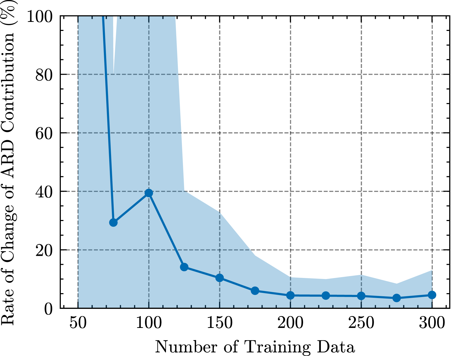

Figure 8 shows the contribution of the uncertain parameters estimated by the ARD kernel to the input of the constructed surrogate model using 300 training datasets. “B” is the bearing, “AS” is the seismic input direction, “K” is the initial stiffness, and “δ ” represents the yield displacement. The first thing to note in this figure is the dominance of the three parameters “AS Cos,” “AS Sin,” and “PGA.” This indicates that the seismic input angle and maximum acceleration of the seismic input contribute significantly. From a structural-dynamics perspective, no problems arise with the seismic input angle, and the maximum acceleration has a significant effect on the maximum response of the bridge system. Although the contributions of “AS Cos,” “AS Sin,” and “PGA” are high, totaling approximately 80%, the contribution of approximately 20% from other uncertain parameters means that they cannot be disregarded. Focusing on the structural parameters, no parameters have significant contributions. However, the contributions of “B71 K,” “B72 K,” “B82 K,” “B83 K,” “B111 K,” and “B112 K″ are relatively noticeable. These parameters are related to the initial stiffness, suggesting that the uncertainty in the initial stiffness is more likely to contribute to the response than the uncertainty in the yield displacement in the seismic-response analysis of curved bridges. By observing the contributions of the input parameters estimated using the ARD kernel, the parameters that contribute to the output response can be identified. The validity of the surrogate model was assessed by verifying that these contributions are significant from an engineering perspective.

Figure 8.

Contribution of input parameters of constructed multi-output GPR surrogate model (Number of training datapoints: 300).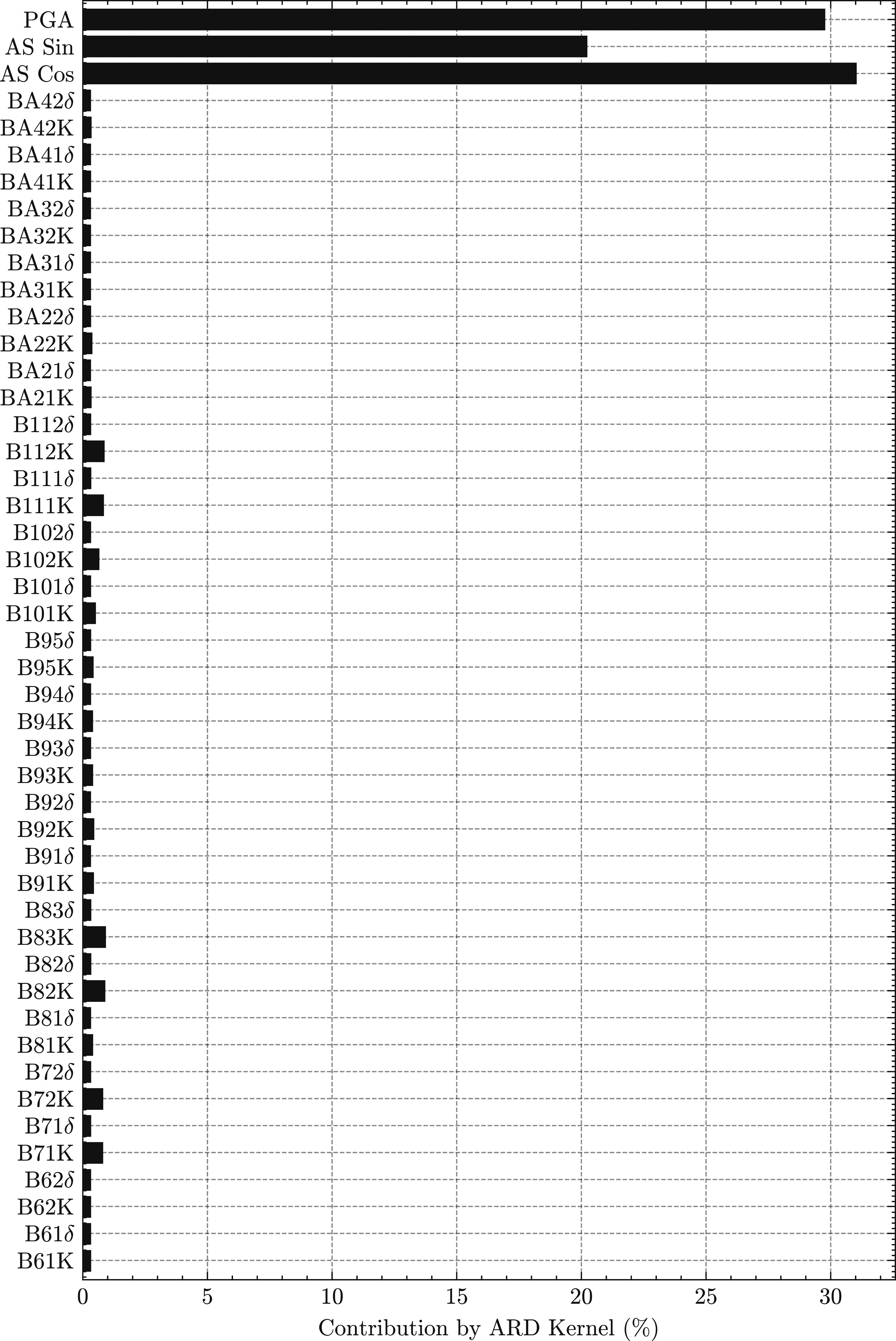

Seismic-fragility analysis using multi-output GPR surrogate model

The fragility analysis of the target bridge system is performed by MC calculations using the multi-output GPR surrogate model constructed in the previous section. Here, 100,000 samples of uncertain parameter sets were created for each PGA, and the failure probability was calculated by applying demand responses, that is, the outputs of the multi-output GPR surrogate model, in equation (12) for the defined limit state. The number of 100,000 samples was confirmed by observing the convergence of the failure probability, which is generally sufficient for deriving one probability distribution in the MC calculation, even considering the dimension of 45. The failure probabilities were derived for 100 PGAs within the range of 0.01 g to 2.00 g with an interval of 0.0199 g. Thus, the number of demand responses used to obtain one fragility curve was 10 million, which is an unrealistic number when conducting FE analysis. For the current bridge case, the nonlinear time-history analysis of each FE model required 10 min to complete. Thus, the benefit of using the surrogate model is evident; the multi-output GPR surrogate model can derive 10 million demand responses in 20 min, which is equivalent to the computational time required by two FE analyses.

The fragility curves of each structural component are shown in Figure 9(a)–(d), for the Slight, Moderate, Extensive, and Collapse limit states, respectively. “B” and “P” represent bearings and piers, respectively. The fragility curves for some components, such as P7 for Slight and P6 for Extensive, approximately followed a lognormal distribution; however, the fragility curves for many components did not follow a lognormal distribution. This supports the need to calculate fragility curves without assuming a lognormal distribution. When the limit-state setting was changed, the fragility-curve shapes of some structural components did not change, whereas others did. This implies that assuming the distribution shape of the fragility curve for each structural member may not be reasonable.

Figure 9.

Fragility curves for structural components. (a) Slight (b) Moderate (c) Extensive (d) Collapse.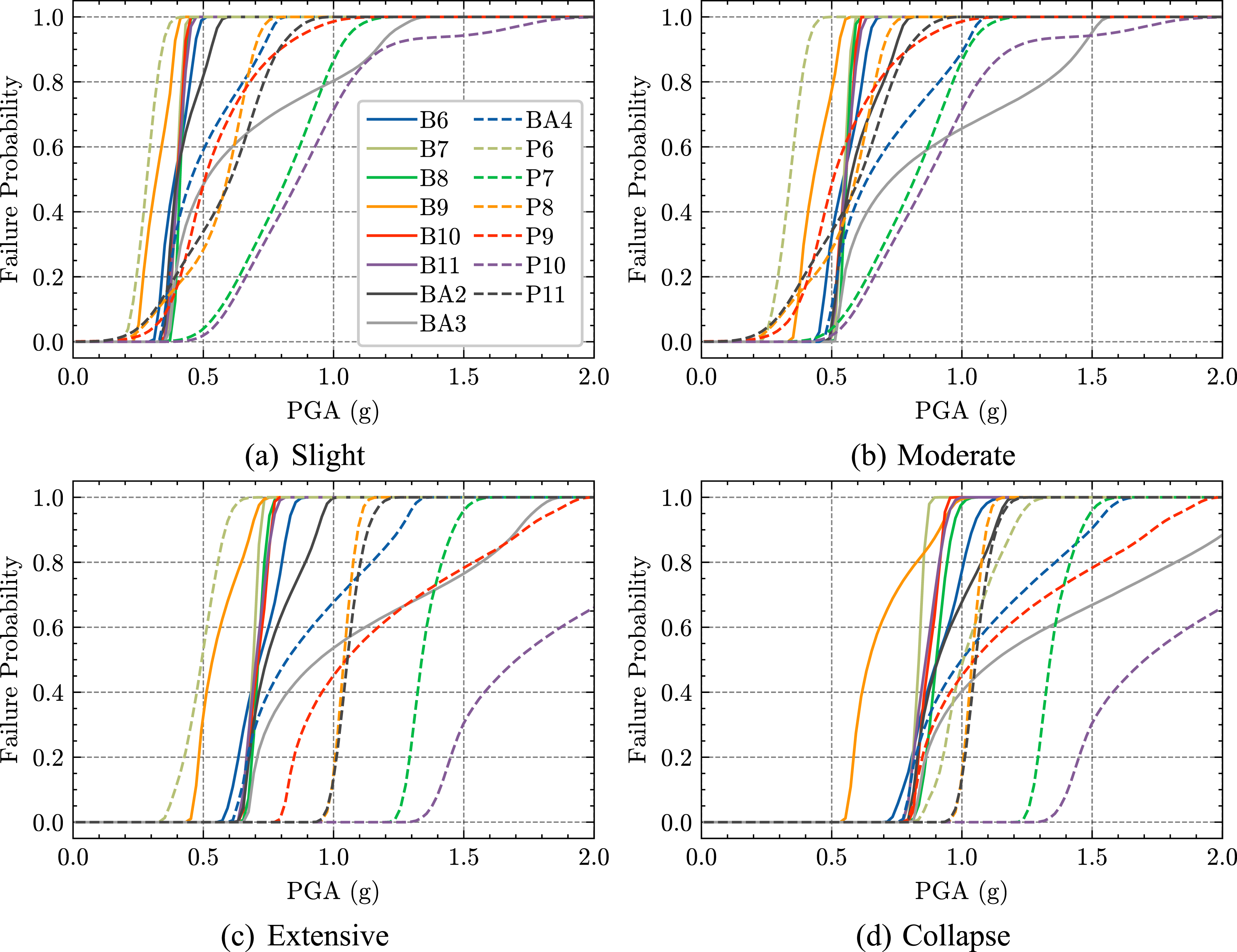

The fragility curves of the system are presented in Figure 10 for “Slight,” “Moderate,” “Extensive,” and “Collapse” limit states. Result shows that, as the PGA increases, the limit states corresponding to Slight, Moderate, Extensive, and Collapse are reached, which is reasonable. The shape of the fragility curve differs depending on the limit state. This can be attributed to the failure modes, which may have changed as the PGA and seismic intensity increased.

Figure 10.

Fragility curve for bridge system.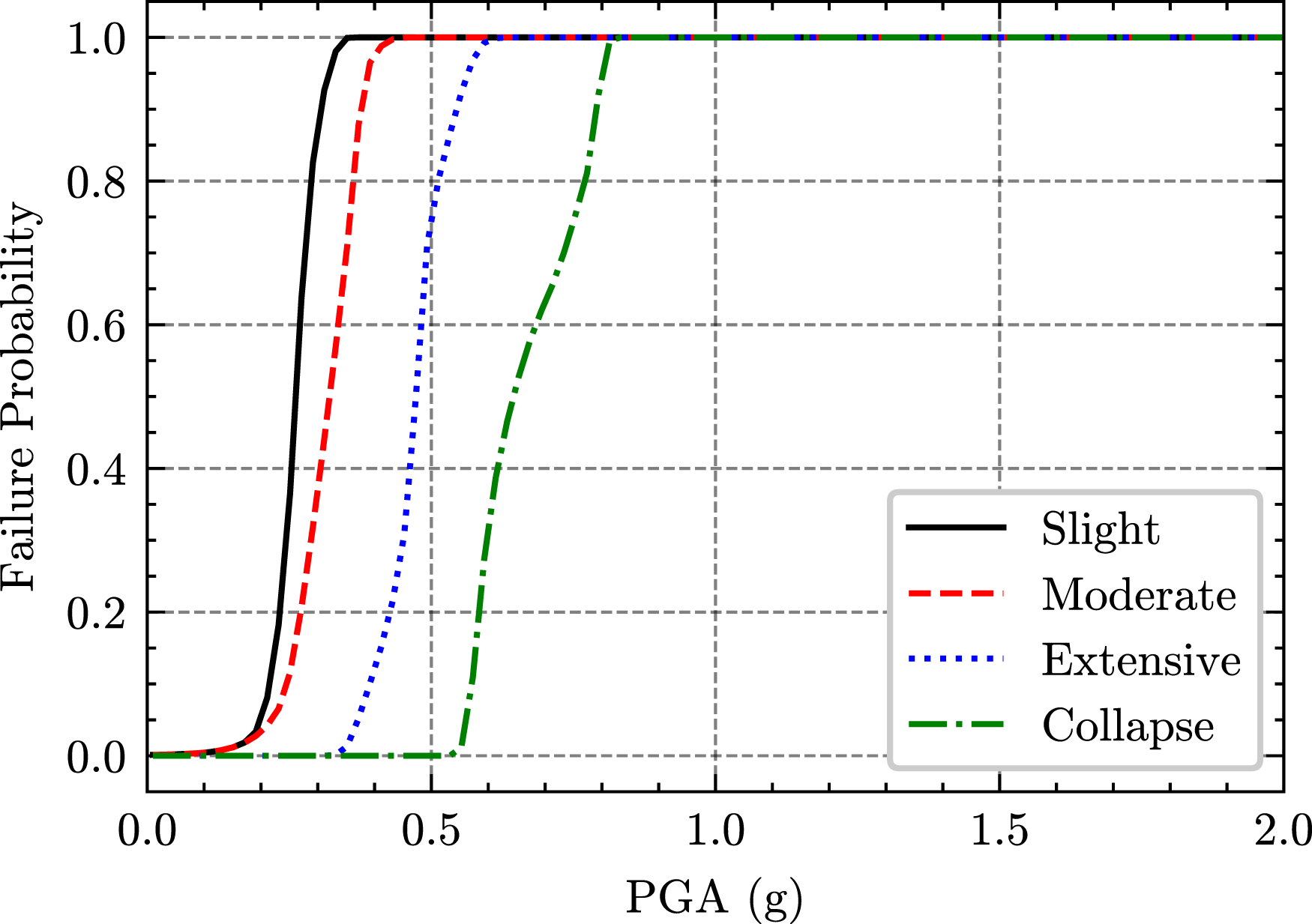

The effect of seismic input direction on the fragility of the bridge system was further investigated. A total of 100,000 points were sampled using the LHS for uncertain parameters other than the PGA and seismic input angle, and calculations were performed for the seismic input angle from 0° to 180° (45° increments) and PGA from 0.01 g to 2.0 g (0.0199 g increments). This implies that the iterative calculations were performed 50 million times (100,000 × 5 × 100). The results of the fragility-curve calculations at 45°, 90°, 135°, and 180° are shown in Figure 11. In Figure 11, the horizontal and vertical axes represent the PGA and failure probability, respectively, and the legend indicates the limit state. Figure 11 shows that, for the Slight, Moderate, and Extensive limit states, the PGA range with the fragility curve does not depend significantly on the seismic input angle. In contrast, as the seismic input angle approaches 90°, the system reaches its Collapse limit state, even when the PGA is in lower range. This indicates that different limit states have different seismic-input directions sensitivity in which the limit state is easily reached.

Figure 11.

Fragility curve of bridge system at different seismic-input directions. (a) 0° (b) 45° (c) 90° (d) 135° (e) 180°.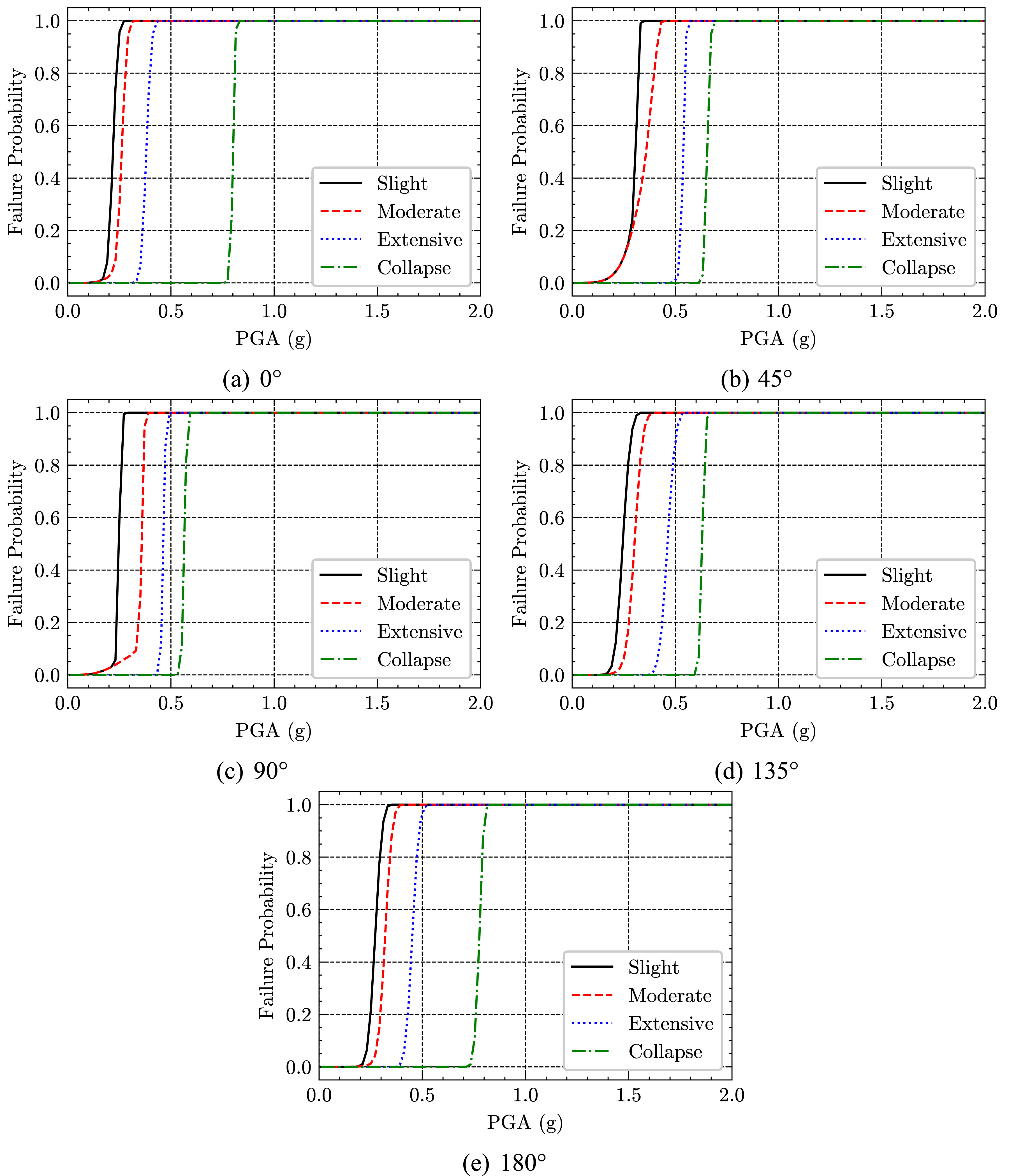

Failure-mode evaluation of bridge system

In this section, the surrogate model constructed in Section 4.1 is used to investigate which structural-component failures contributed to the failure of the bridge system. The surrogate model is constructed using 300 training datapoints, as described in the previous section. The 100,000 samples of the set of uncertain parameters, except PGA, were created for each PGA with an increment of 100 in the range from 0.01 g to 2.0 g by the LHS; thus, 10 million iterations of numerical analysis were performed. The results of the failure-mode evaluations, that is, the structural components that contributed to the failure of the bridge system, are shown in Figure 12. The horizontal axis represents the failure probability of the bridge system and the vertical axis represents the ratio of the failed structural components that contribute to the system failure for each probability. The lines in Figure 12 indicate each component, as shown in the legend of Figure (d), where “B” indicates bearings and “P” indicates piers. Figure 12 shows that “P6,” that is, RC piers, had a high failure contribution rate for “Slight,” “Moderate,” and “Extensive” bridge-system failures. However, for the “Collapse” limit state, the failure of “B9,” that is, the failure of the bearings on pier 9, caused the system failure. In Figure 4, P6 and B9 are locations with large mode displacements, which is reasonable from a structural-vibration perspective. Additionally, for all limit states the rate of structural components that fail changes during failure. This indicates that the failure mode changes as the PGA increases.

Figure 12.

Component failure ratio for failure of bridge system. (a) Slight (b) Moderate (c) Extensive (d) Collapse.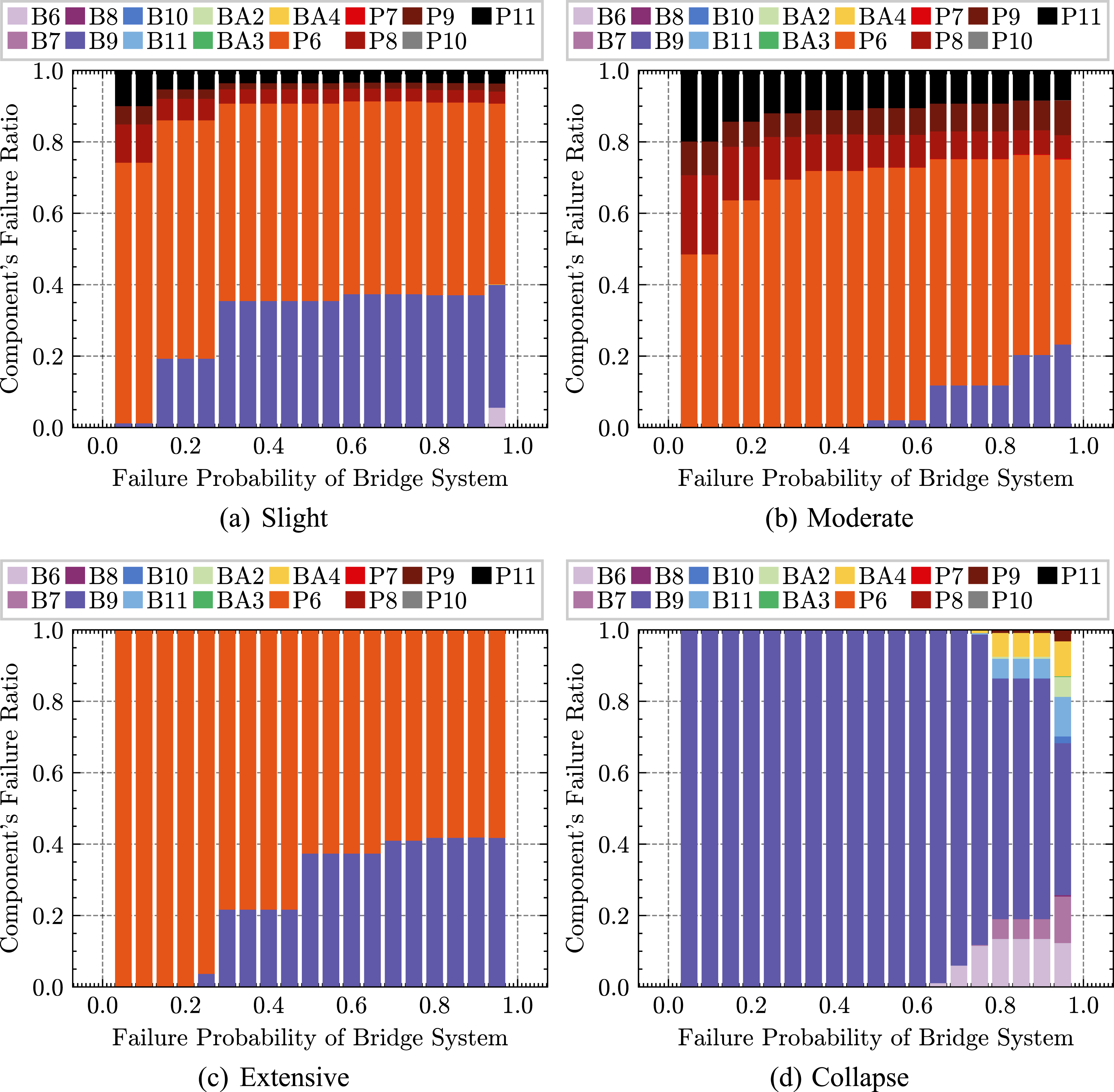

Next, the failure ratios of structural components to the bridge system were investigated to observe how they vary with the angle of seismic input. The relationship between the seismic input angle and the failure ratio of structural components for a bridge system is shown in Figure 13 when the failure probability of the system is 0.5, that is, 50%. The horizontal axis is the seismic input angle, and the vertical axis is the ratio of the failed structural components when the system fails at each angle. As shown in Figure 13, the failure mode varies with the seismic input angle for all limit states. When the limit states are Slight and Moderate, most failures occur at B9 and P6, with larger failure ratios at P8, P9, and P11 at seismic input angles of 50° and approximately 200°–280°. This indicates that the failure of bearings and RC piers often causes system failure, but some steel piers fail at certain seismic input angles. When the limit state is Extensive, the B9 and P6 failure ratios dominate, regardless of the seismic input angle. However, the failure ratios change with the seismic input angle. When the limit state is Collapse, the failure ratio at B9 is dominant; however, depending on the seismic input angle, the failure at B9 does not contribute to system failure. This indicates that the failure mode varies significantly depending on the seismic input angle. Additionally, P6, which has failures in other limit states, has an almost zero failure ratio during Collapse. This indicates that different limit states have different structural components that contribute to the system failure. In addition, for all limit states, the failure of B9 is observed at seismic input angles of approximately 90° and 270°. For the effective masses in Table 2, m-Mode one dominates in the 90° and 270° directions, that is, along the Z-axis. For the modal shapes shown in Figure 4, the displacements near B9 are large in mode 1. Thus, the dominance of mode one is considered to destroy B9. This verification shows that the failure mode of the bridge varies significantly, depending on the seismic input angle and limit-state setting. Because the surrogate model is much faster than the FE analysis, a detailed evaluation, such as determining the influence of the seismic input angle and which components failed, becomes possible.

Figure 13.

Component failure ratio versus angle of seismic input. (a) Slight (b) Moderate (c) Extensive (d) Collapse.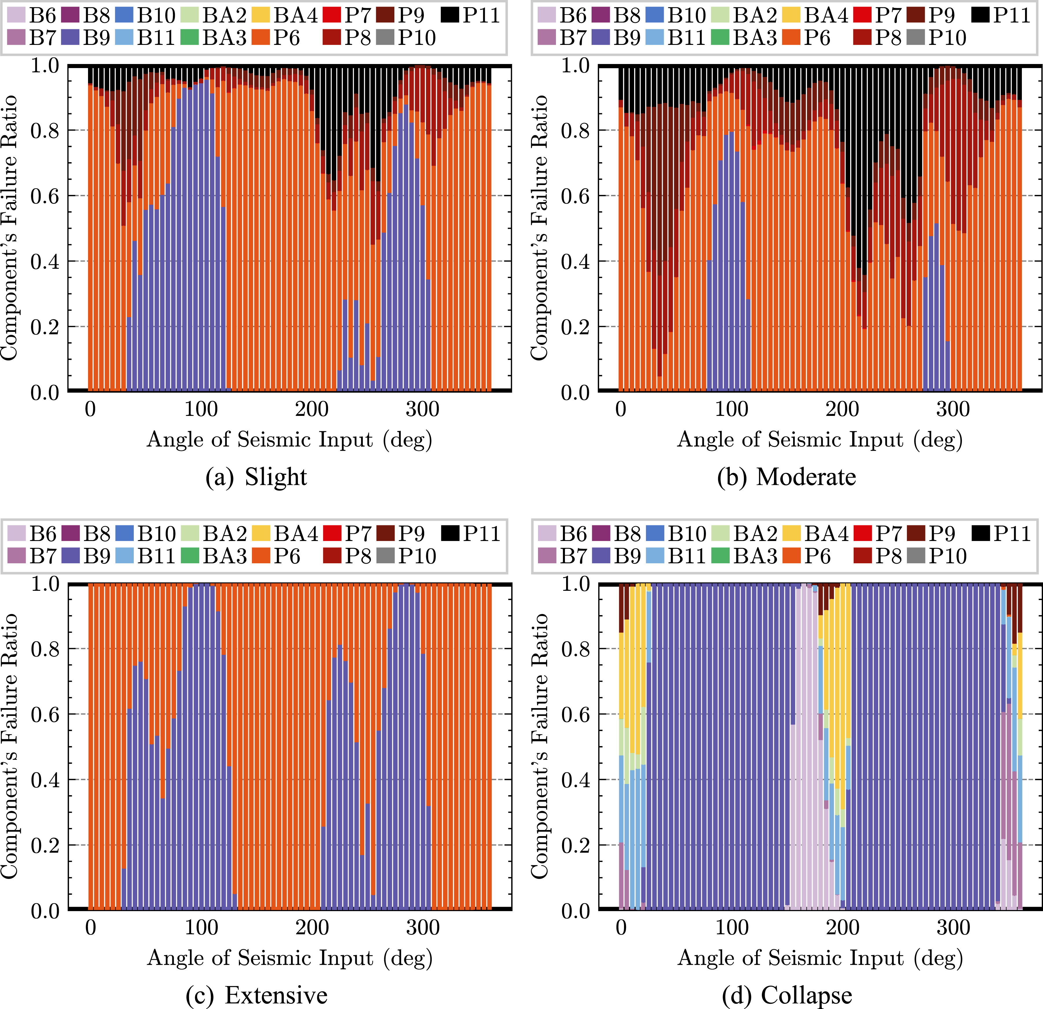

Conclusions

This study presents a multi-output GPR surrogate model for the seismic-fragility analysis of bridge structural systems. As the multi-output GPR can model correlations among outputs, high accuracy and effective computational-cost reduction are expected when constructing a surrogate model for structural fragility analysis, which requires the evaluation of multiple demand responses. In addition, the explainability of the constructed surrogate model is implemented by adopting the ARD kernel, which indicates the contribution of the input-parameter uncertainties to the outputs. The fragility analysis using the multi-output GPR surrogate model was verified by applying it to a seismic isolation highway bridge with multiple spans. Some significant results and conclusions are summarized below:

1. The multi-output GPR surrogate model demonstrated high accuracy and stability in predicting the seismic responses of the bridge components. The model achieved a coefficient of determination R² of over 0.98 in all outputs of demand responses with 300 training datapoints. Compared to the typical GPR, these high performances were achieved with less training data. This was considered because the multi-output GPR appropriately modeled the correlations among the outputs.

2. The multi-output GPR surrogate model significantly reduced the computational time of the fragility analysis. The constructed surrogate model can provide 10 million demand responses in approximately 20 min, which is almost the same time required for two runs of nonlinear time-histories using the FE model.

3. The ARD kernel adopted in the multi-output GPR model was used to derive the contribution of each input-parameter uncertainty to the outputs. In the verification of the bridge, the uncertainty in the property of the seismic load, that is, the direction of the input to the bridge, was identified as the most influential parameter, except for the intensity of the seismic load. In addition, the initial stiffness of the rubber bearings at some piers contributed slightly more to the structural properties.

4. Seismic-fragility curves at both the component and system levels were appropriately obtained via Monte Carlo calculations using a multi-output GPR surrogate model with a sufficient number of samples. The Monte Carlo calculation-based fragility analysis could derive an arbitrary probability distribution of the fragility curve because no assumption is required for the stochastic model for each input-parameter uncertainty.

5. System-fragility analysis with a sufficient number of samples in the Monte Carlo calculation realized by the multi-output GPR surrogate model enabled a detailed evaluation of the failure modes, identifying which structural components contributed to the system failure. The failed structural component varied with the seismic input angle, indicating the relationships between the structural dynamic characteristics of the bridge and seismic input characteristics.

The effectiveness of the multi-output GPR surrogate model with explainability for the seismic-fragility analysis of a bridge system was demonstrated; however, some limitations exist, leading to potential future work. First, a large amount of training data (at least 100 datapoints) is required to obtain an accurate and stable surrogate model. This implied that more than 100 FE-analysis runs were required. While this also depends on the dimensions of inputs and outputs (46 inputs and 28 output dimensions in this study), the surrogate model trained by 300 datapoints was adopted for verification. Additional ideas for reducing the amount of training data, such as the application of adaptive sampling, should be considered in future studies. Regarding the uncertainties to be considered in seismic-fragility analysis, those of seismic waveforms should be included. Dealing with the high-dimensional features of seismic waveforms is challenging; however, future work can address this by implementing the feature extraction of seismic waveforms by integrating deep learning with GPR.

In conclusion, the results showed that the multi-output GPR surrogate model that implements explainability via the ARD kernel is effective for an appropriate Monte Carlo calculation-based seismic-fragility analysis of a bridge structural system. This approach not only enhanced the performance of the surrogate model, but also provided a statistically significant understanding of the failure mode of the system failure, which may be valuable in seismic design, the reinforcement of the retrofit of existing bridges, and the resilience enhancement of structural systems.

Footnotes

Declaration of conflicting interests

The author(s) declared no potential conflicts of interest with respect to the research, authorship, and/or publication of this article.

Funding

The author(s) disclosed receipt of the following financial support for the research, authorship, and/or publication of this article: This study was supported by the JST FOREST Program, Japan [grant number: JPMJFR205T].

ORCID iD

Taisei Saida

References

Abbiati

Broccardo

Abdallah

, et al. (2021) Seismic fragility analysis based on artificial ground motions and surrogate modeling of validated structural simulators. Earthquake Engineering & Structural Dynamics 50(9): 2314–2333.

Bichon

Eldred

Swiler

, et al. (2008) Efficient global reliability analysis for nonlinear implicit performance functions. AIAA Journal 46(10): 2459–2468.

Billah

Alam

(2015) Seismic fragility assessment of highway bridges: a state-of-the-art review. Structure and Infrastructure Engineering: Maintenance, Management, Life-Cycle Design and Performance 11(6): 804–832.

Bonilla

Chai

Williams

(2007) Multi-task Gaussian process prediction. In: Advances in neural information processing systems 20. proceedings.neurips.cc.

Bucher

Bourgund

(1990) A fast and efficient response surface approach for structural reliability problems. Structural Safety 7(1): 57–66.

Cao

X-Y

Feng

D-C

Beer

(2023) Consistent seismic hazard and fragility analysis considering combined capacity-demand uncertainties via probability density evolution method. Structural Safety 103: 102330.

Capacci

Biondini

Frangopol

(2022) Resilience of aging structures and infrastructure systems with emphasis on seismic resilience of bridges and road networks: review. Resilient Cities and Structures 1(2): 23–41.

Chojaczyk

Teixeira

Neves

, et al. (2015) Review and application of Artificial Neural Networks models in reliability analysis of steel structures. Structural Safety 52: 78–89.

Echard

Gayton

Lemaire

(2011) AK-MCS: an active learning reliability method combining Kriging and Monte Carlo Simulation. Structural Safety 33(2): 145–154.

10.

Federal Emergency Management Agency, Hazus 5.1 (2021) Hazus Earthquake Model Technical Manual.

11.

FORUM8 (2019) Civil & Structural Engineering - FORUM8 - 3D VR & Visual Interactive Simulation. Available at: https://www.forum8.com/solutions/engineers-studio/ (accessed 9 January 2023).

12.

Gardner

Pleiss

Bindel

, et al. (2018) GPyTorch: blackbox Matrix-matrix Gaussian process inference with GPU acceleration In: Advances in Neural Information Processing Systems, 28 September 2018, Curran Associates, Inc. Available at: https://proceedings.neurips.cc/paper/2018/hash/27e8e17134dd7083b050476733207ea1-Abstract.html (accessed 7 January 2023).

13.

Golparvar

Papadopoulos

Ezzat

, et al. (2021) A surrogate-model-based approach for estimating the first and second-order moments of offshore wind power. Applied Energy 299: 117286.

14.

Hawchar

El Soueidy

C-P

Schoefs

(2017) Principal component analysis and polynomial chaos expansion for time-variant reliability problems. Reliability Engineering & System Safety 167: 406–416.

15.

Japan Road Association (2016) Specifications for highway bridges part v seismic design. Tokyo, Japan: Japan Road Association.

16.

Karamlou

Bocchini

(2015) Computation of bridge seismic fragility by large-scale simulation for probabilistic resilience analysis. Earthquake Engineering & Structural Dynamics 44(12): 1959–1978.

17.

Kim

J-S

Park

W-S

Han

T-S

(2021) Framework to evaluate seismic fragility of bridges considering component damage correlations. Journal of Earthquake and Tsunami 15(05): 2150022.

18.

Kim

S-R

Song

(2023) Estimation of first-passage probability under stochastic wind excitations by active-learning-based heteroscedastic Gaussian process. Structural Safety 100: 102268.

19.

Kingma

(2014) Adam: A Method for Stochastic Optimization. arXiv [cs.LG]. Available at: https://arxiv.org/abs/1412.6980.

20.

Caracoglia

(2020) A neural network surrogate model for the performance assessment of a vertical structure subjected to non-stationary, tornadic wind loads. Computers & Structures 231: 106208.

21.

Linardatos

Papastefanopoulos

Kotsiantis

(2020) Explainable ai: a review of machine learning interpretability methods. Entropy 23(1).

22.

Lundberg

Lee

S-I

(2017) A unified approach to interpreting model predictions. In: Advances in Neural Information Processing Systems 30. proceedings.neurips.cc.

23.

Mackie

Stojadinović

(2005) Fragility Basis for California Highway Overpass Bridge Seismic Decision Making. Pacific Earthquake Engineering Research Center, College of Engineering, University of California, Berkeley. Available at: https://play.google.com/store/books/details?id=u4wpqAAACAAJ.

24.

Marelli

Sudret

(2018) An active-learning algorithm that combines sparse polynomial chaos expansions and bootstrap for structural reliability analysis. Structural Safety 75: 67–74.

25.

Montazeri

Ghodrati Amiri

Namiranian

(2021) Seismic fragility and cost-benefit analysis of a conventional bridge with retrofit implements. Soil Dynamics and Earthquake Engineering 141: 106456.

26.

Nielson

DesRoches

(2007) Seismic fragility methodology for highway bridges using a component level approach. Earthquake Engineering & Structural Dynamics 36(6): 823–839.

27.

Padgett

DesRoches

(2008) Methodology for the development of analytical fragility curves for retrofitted bridges. Earthquake Engineering & Structural Dynamics 37(8): 1157–1174.

28.

Patil

Jung

Kwon

O-S

(2016) Structural performance of a parked wind turbine tower subjected to strong ground motions. Engineering Structures 120: 92–102.

29.

Rashid

Nishio

(2023) System fragility evaluation of a curved highway bridge structure considering multi-direction seismic excitations. Advances in Structural Engineering 26: 13694332231198136.

30.

Rasmussen

(2004) Gaussian processes in machine learning. In: Bousquet

von Luxburg

Rätsch

(eds) Advanced Lectures on Machine Learning: ML Summer Schools 2003, Canberra, Australia, February 2 - 14, 2003, Tübingen, Germany, August 4 - 16, 2003, Revised Lectures. Berlin, Heidelberg: Springer Berlin Heidelberg, 63–71. Available at: DOI: 10.1007/978-3-540-28650-9_4.

31.

Rocco

Moreno

(2002) Fast Monte Carlo reliability evaluation using support vector machine. Reliability Engineering & System Safety 76(3): 237–243.

32.

Roy

Manna

Chakraborty

(2019) Support vector regression based metamodeling for structural reliability analysis. Probabilistic Engineering Mechanics 55: 78–89.

33.

Saida

Nishio

(2023) Transfer learning Gaussian process regression surrogate model with explainability for structural reliability analysis under variation in uncertainties. Computers & Structures 281: 107014.

34.

Sainct

Feau

Martinez

J-M

, et al. (2020) Efficient methodology for seismic fragility curves estimation by active learning on Support Vector Machines. Structural Safety 86: 101972.

35.

Selvaraju

Cogswell

Das

, et al. (2016) Grad-CAM: visual explanations from deep networks via Gradient-based localization. In: Proceedings of the IEEE International Conference on Computer Vision, 7 October 2016, pp. 618–626. Available at: https://openaccess.thecvf.com/content_iccv_2017/html/Selvaraju_Grad-CAM_Visual_Explanations_ICCV_2017_paper.html (accessed 22 February 2023).

36.

Shan

Deng

(2020) Seismic fragility analysis of irregular bridges with non-circular tall piers considering ground motion directionality. Bulletin of Earthquake Engineering 18(4): 1723–1753.

37.

Skandalos

Chakraborty

Tesfamariam

(2022) Seismic reliability analysis using a multi-fidelity surrogate model: example of base-isolated buildings. Structural Safety 97: 102222.

38.

Takeda

Sozen

Nielsen

(1970) Reinforced concrete response to simulated earthquakes. Journal of the Structural Division 96(12): 2557–2573.

39.

Thapa

Shrestha

Gautam

(2022) Seismic fragility analysis of RC bridges in high seismic regions under horizontal and simultaneous horizontal and vertical excitations. Structures 37: 284–294.

40.

Wada

Hirose

(1989) Building frames subjected to 2D earthquake motion. Seismic Engineering: Research and Practice Proceedings. San Francisco, CA: Structures Congress, 388–397.

41.

Wang

Liu

(2018) Multivariate probabilistic seismic demand model for the bridge multidimensional fragility analysis. KSCE Journal of Civil Engineering 22(9): 3443–3451.

42.

Wei

Yang

Jiang

, et al. (2018) Effects of uncertain characteristic periods of ground motions on seismic vulnerabilities of a continuous track–bridge system of high-speed railway. Bulletin of Earthquake Engineering 16(9): 3739–3769.

43.

Wei

, et al. (2020) Evaluation of optimal ground motion intensity measures and seismic fragility analysis of a multi-pylon cable-stayed bridge with super-high piers in Mountainous Areas. Soil Dynamics and Earthquake Engineering 129: 105945.

44.

Williams

CKI

Rasmussen

(1995) Gaussian processes for regression. In: Advances in Neural Information Processing Systems. proceedings.neurips.cc. forthcoming 1995.

45.

Yang

C-SW

Werner

DesRoches

(2015) Seismic fragility analysis of skewed bridges in the central southeastern United States. Engineering Structures 83: 116–128.

46.

Yang

Yuan

Zhong

, et al. (2023) Near-fault pulse seismic ductility spectra for bridge columns based on machine learning. Soil Dynamics and Earthquake Engineering 164: 107582.

47.

Yoshida

Nakamura

S-K

(2023) Bayesian updating of model parameters using adaptive Gaussian process regression and particle filter. Structural Safety 102: 102328.

48.

Zhang

Huo

(2009) Evaluating effectiveness and optimum design of isolation devices for highway bridges using the fragility function method. Engineering Structures 31(8): 1648–1660.

49.

Zhong

Pang

Jeon

J-S

, et al. (2016) Seismic fragility assessment of long-span cable-stayed bridges in China. Advances in Structural Engineering 19(11): 1797–1812.

50.

Zhong

Wan

H-P

Yuan

, et al. (2020) Risk-informed sensitivity analysis and optimization of seismic mitigation strategy using Gaussian process surrogate model. Soil Dynamics and Earthquake Engineering 138: 106284.

51.

Zhong

Zhu

Zheng

, et al. (2023) Multivariable probabilistic seismic demand models for parametric fragility prediction of isolated bridges portfolios under pulse-like GMs. Engineering Structures 292: 116517.

System fragility analysis of highway bridge using multi-output Gaussian process regression surrogate model

Abstract

Keywords

Introduction

Multi-output GPR surrogate modeling for seismic-fragility analysis

Multi-output Gaussian process regression

ARD kernel in GPR and estimation of contributions to outputs

Calculating fragility curve and estimating component contributing to system fragility

Seismic fragility evaluation of seismic isolation highway bridge

FE modeling for seismic-response analysis

Uncertainties considered in fragility analysis and inputs-outputs of surrogate model

Limit-state definitions for bridge components and system

Results of surrogate modeling for seismic fragility analysis

Accuracy of multi-output GPR surrogate model

Explainability of constructed multi-output GPR surrogate model

Seismic-fragility analysis using multi-output GPR surrogate model

Failure-mode evaluation of bridge system

Conclusions

Footnotes

Declaration of conflicting interests

Funding

ORCID iD

References