Sage Journals: Discover world-class research

Abstract

The United States has many aging bridges, mostly designed with outdated 1950s standards and now facing overloading issues due to heavier modern vehicles. Assessing these bridges' conditions and updating safe load capacities are essential. This paper proposes using acoustic emission (AE) to predict vehicle loads on prestressed concrete girder bridges, potentially supplementing traditional weigh-in-motion (WIM) sensor methods. Three enhanced machine learning techniques: balanced training artificial neural network (BT-ANN), balanced training random forest (BT-RF), and balanced training AdaBoost (BT- AdaBoost) were developed for AE data analysis, addressing training imbalances with an ensemble strategy. The study involved a full-scale flexural test on nine prestressed concrete girders, treating load determination as a classification task. AE signals were categorized into corresponding load steps. The results demonstrate that the proposed BT-RF performs well in classifying AE signals into their respective load steps. Additionally, this paper investigates and discusses the robustness of the BT-RF model.

Keywords

prestressed concrete girder acoustic emission structural health monitoring artificial neural network AdaBoost random forest

Introduction

Bridges serve as a fundamental component in the infrastructure matrix, both within the United States and internationally. The state of South Carolina is particularly dependent on its extensive array of bridges, which are vital for ensuring community interconnectivity, as well as enabling commercial activities and transportation. Ranked 26th in the country for its bridge inventory, South Carolina maintains more than 9,000 bridges. Most of these structures were originally engineered to comply with H-10 or H-15 load specifications. However, these specifications are surpassed by the more rigorous demands of the contemporary HL-93 load standard (Aashto, 1998; Hearn, 2014). The South Carolina Department of Transportation (SCDOT) manages approximately 90% of all bridges. On average, the bridges are approximately 40 years old, approaching the 50-years service level, with 6.8% being load posted, 11% being structurally deficient, and 0.33% being reported closed (Elbatanouny, 2023). This is a direct outcome of bridge deterioration and overloading due to long service life and increased vehicle loads.

Bridges undergo systematic inspections aimed at assessing the state of their structural elements. Furthermore, these evaluations ascertain whether the bridges have sufficient residual structural strength to withstand expected live loads along with an appropriate factor of safety. Should the residual structural capacity prove inadequate for the projected live load demands, strategies including load posting, structural rehabilitation, or even bridge closure might be imperative to ensure the safety of the public. Consequently, the process of load rating stands as an essential resource management instrument that bridge proprietors utilize to gauge the differential between expected live loads and the bridges’ residual structural capacity (Hou et al., 2022).

The variability in bridge loads, predominantly influenced by live loads, presents considerable uncertainty. To mitigate this, the acquisition of site-specific traffic data for evaluating live loads is a recognized method (Uddin et al., 2011). Therefore, weigh-in-motion (WIM) systems are strategically positioned at various points to record the loads of vehicles traversing bridges. The most common types of WIM sensors available in the market include piezoelectric, load cell, and bending plate technologies. However, these systems are not without limitations: WIM systems employing load cells tend to have substantial cross-sectional areas; bending plate sensors can be onerous to install; and piezoelectric sensors, while useful for traffic data collection, are incapable of measuring weight (Dontu et al., 2020; Mihaila et al., 2022). Moreover, the integration of WIM sensors into road surfaces requires lane closures, often extending over a week, which can be particularly disruptive for certain bridges. Consequently, there is a significant need to explore the development of compact, effective, and light-weight sensors for vehicle load measurement that can be installed on bridges with minimal disruption and expedience.

Many different types of sensors have been utilized for the structural health monitoring of structures as sensor technology has advanced (Tan et al., 2021, 2022; Zhu et al., 2021). For instance, Acoustic Emission (AE) sensors are extensively employed owing to their user-friendly operation, high sensitivity to damage, and capacity for continuous structural response monitoring (Elhussien Elbatanouny et al., 2024; Soltangharaei et al., 2020). With an array of piezoelectric sensors, AE detects the elastic waves generated by crack formation and growth. Structural damage can be detected and localized by AE emissions before it becomes visible at the surface of an element (Vandecruys et al., 2022). AE parameters were analyzed to assess structural damage, including crack detection, crack location, crack type, and corrosion (Mohamed K ElBatanouny et al., 2014a; Li et al., 2023). Measuring the vehicle loads while concurrently monitoring the bridge will be a great advantage as it saves time and money through its relatively easy installation.

Researchers analyzed AE data using various methods and parameters (Aggelis et al., 2013; Bahari et al., 2017; Zhou et al., 2021). Statistical analyses for the AE parameters were utilized to evaluate and monitor the condition of bridge components. The validity of damage assessment of prestressed concrete I-beams using conventional AE parameter-based methodology was examined by (Zeng et al., 2020). A four-point bending test was carried out on a full-scale I-section prestressed concrete beam. To assess the response of the beam in terms of damage formation, the variance in AE signal activity throughout incremental loading cycles was analyzed. In addition, (Worley et al., 2019) investigated the potential of AE sensing techniques for crack detection and localization in prefabricated prestressed concrete girders. The results indicated that AE sensing could be applied as a quality control procedure for prefabricated bridge elements.

Although many AE parameters are gathered, statistical analysis depends on a single parameter or correlation plots of two parameters. Hence, some information on the signals may be lost, resulting in a failure to make a strategic decision and lower productivity (Ma and Du, 2020). Several AE parameters should be considered simultaneously to overcome this limitation (Holford et al., 2017; Soltangharaei1a et al., 2020).

A variety of machine learning methodologies, including artificial neural network (ANN), AdaBoost, and random forest, have been implemented to concurrently analyze multiple AE parameters. Machine learning constitutes a supervised approach to intelligent data analysis (Jordan and Mitchell, 2015), capable of discerning data patterns and formulating decisions through the analysis of features extracted from the dataset (H Wang et al., 2016).

(Nair et al., 2020) monitored the damage modes in CFRP-strengthened concrete structures. The main sources of AE activities were identified based on visual observation and damage mechanism expectation. AE data was clustered using the unsupervised k-means technique. Each cluster was associated with one or more damage mechanisms. The ANN models, support vector machines (SVM), and multilayer perceptron (MLP) algorithms were then trained using the classified AE data. Finally, the trained models were applied to identify the damage in similar specimens. The results pointed out the high performance of classification rates for both algorithms. (Ai et al., 2021b) developed an automated impact detection system for aircraft components utilizing AE and machine learning algorithms. The authors employed ANN and AdaBoost algorithms. The results show that AdaBoost performed better than ANN in localizing the impact. (Ai et al., 2021a) conducted a study to localize cracking on dry cask storage system canisters. The authors employed three machine learning algorithms (ANN, random forest, and stacked autoencoders) to analyze the AE data. The results revealed that the random forest method outperformed the ANN algorithm, with an accuracy of 91.5% for the random forest and 80% for the ANN. These studies demonstrate the capacity of machine learning algorithms in the field of AE monitoring.

In a recent study, (Laxman et al., 2023) explored the application of Acoustic Emission (AE) techniques for the estimation of vehicular loads on bridge structures. The investigation was conducted using two precast flat slabs subjected to a four-point bending test. The research team implemented an Artificial Neural Network (ANN) algorithm, evaluating 13 distinct AE parameters in tandem. Findings from the study demonstrated the capability of the ANN to effectively categorize AE signals in correlation with specific vehicle loads, achieving a satisfactory level of precision. However, in this study, the classification was done on two load steps with a step size of 10 kip, and only the ANN algorithm was implemented. Moreover, this study is limited to precast RC flat slab bridges. Using AE to predict the vehicle loads on other typical bridges, such as girder bridges, was not studied.

The current study explores an improved load determination method for girder bridges based on previous work (Laxman et al., 2023). Flexural tests were performed on prestressed concrete girders to simulate vehicle loads. AE data was collected and analyzed from four load steps with a step size of four kip. In addition, various machine learning algorithms, ANN, AdaBoost, and random forest, were investigated. The main contribution of this paper is to develop an optimized method for predicting vehicle loads that pass over girder bridges from the collected AE data. Information on traffic loads can help transportation networks operate more efficiently and cost-effectively (Lydon et al., 2016).

The remaining sections of this paper are arranged as follows. First, the experimental setup is presented in Section 2. Next, the data preprocessing and methodology are presented in Section 3. Section 4 details the results and discussion. Finally, section 5 provides a summary of the conclusions and recommendations.

Experimental setup

Specimens

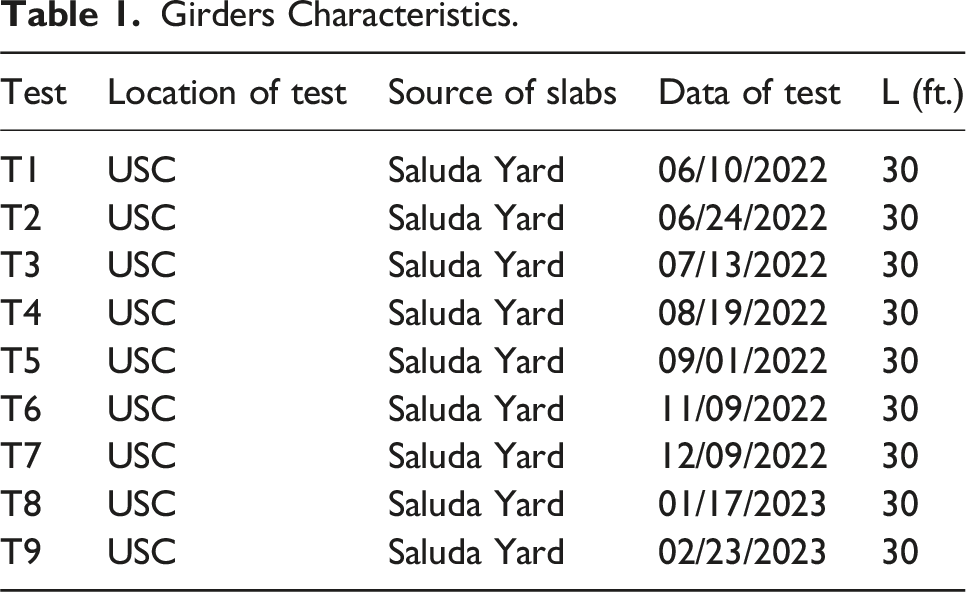
A series of flexural experiments were performed on nine prestressed concrete girders (Table 1). These girders had originally been part of bridges with a span of 30-ft, constructed in the 1960s, which were subsequently dismantled after three decades of utilization and then stored at an SCDOT facility. Figure 1 illustrates the geometrical specifications and the reinforcement layout of the girders. The reinforcement design, according to SCDOT schematics, includes longitudinally placed five No. 3 bars and ten 3/8-inch diameter prestressing strands. The strands exhibit a downward curvature at the midpoint except for the lowest strand, as shown in Figure 1. Upon initial tensioning, the lowest strand received a prestressing force of 14,000 pounds for each segment, whereas the upper four strands each received a prestressing force of 13,450 pounds. The cross reinforcement comprised No. 4 bars positioned at intervals of 12 inches center-to-center, along with No. Four stirrups at similar spacings. The concrete’s designated compressive strength and the deformed steel bars' yield strength were specified as 5,000 psi and 40,000 psi, respectively, with the prestressing strands having an ultimate strength of 250,000 psi Table 1.

Figure 1.

Dimensions and reinforcement details of girders.

Table 1.

Girders Characteristics.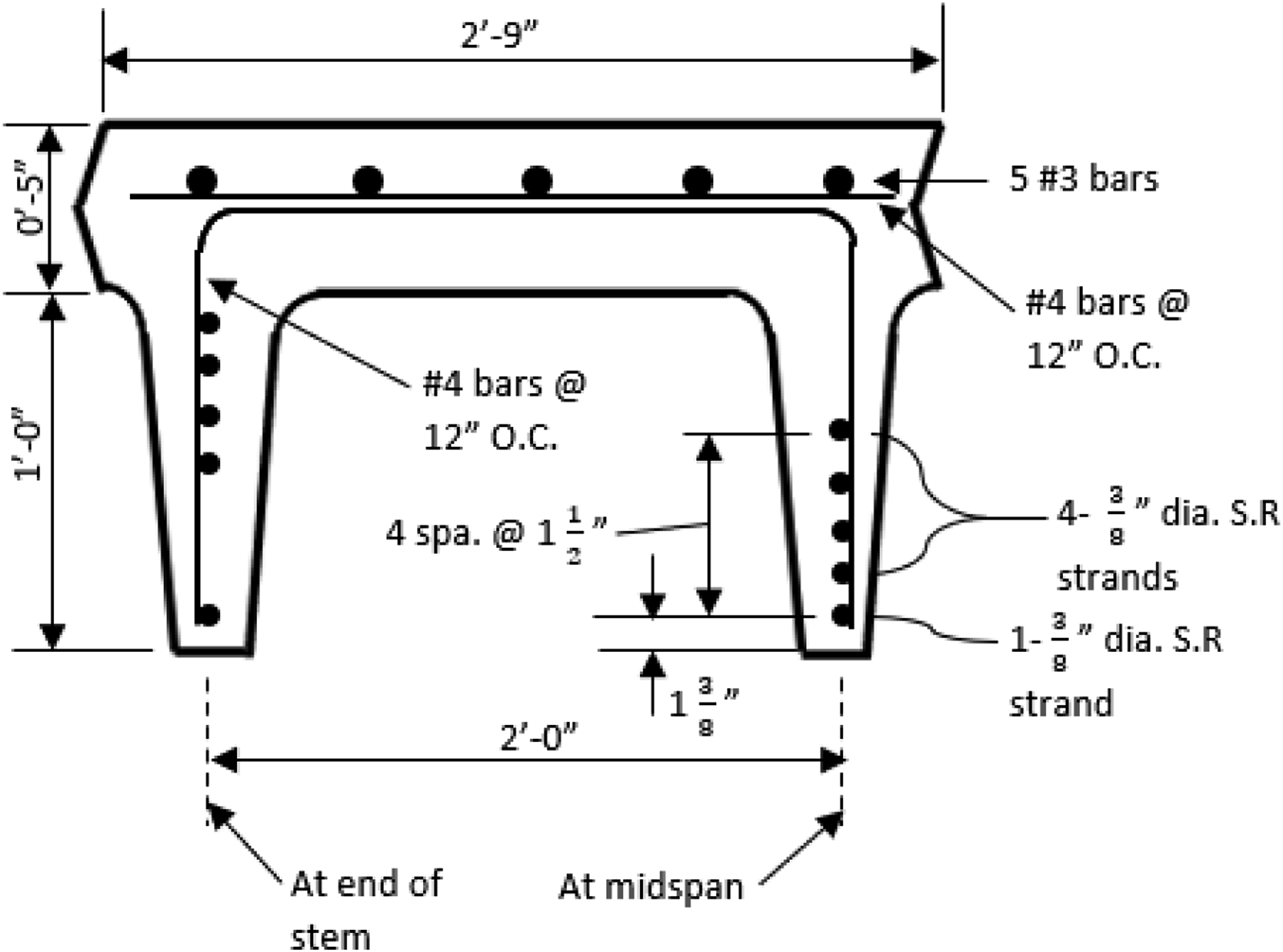

Test	Location of test	Source of slabs	Data of test	L (ft.)
T1	USC	Saluda Yard	06/10/2022	30
T2	USC	Saluda Yard	06/24/2022	30
T3	USC	Saluda Yard	07/13/2022	30
T4	USC	Saluda Yard	08/19/2022	30
T5	USC	Saluda Yard	09/01/2022	30
T6	USC	Saluda Yard	11/09/2022	30
T7	USC	Saluda Yard	12/09/2022	30
T8	USC	Saluda Yard	01/17/2023	30
T9	USC	Saluda Yard	02/23/2023	30

Test setup

Flexural tests were conducted to simulate the effect of a vehicle passing over the bridge girders. Nine 30-foot long, simply supported girders were subjected to a four-point bending tests in the lab. at the University of South Carolina (USC). Figure 2 shows schematics of the test setup. The girders were placed over nine inchwide neoprene bearing pads above the supports to lessen friction during the application of the load. Two structural steel members support the spreader beam, each resting on two neoprene bearing pads to establish four contact points. These contact points are designed to rest directly over the girder legs and create a four-point bending test setup, as shown in Figure 2. The center of one support to the other is 27 ft. long.

Figure 2.

Test setup of the girders.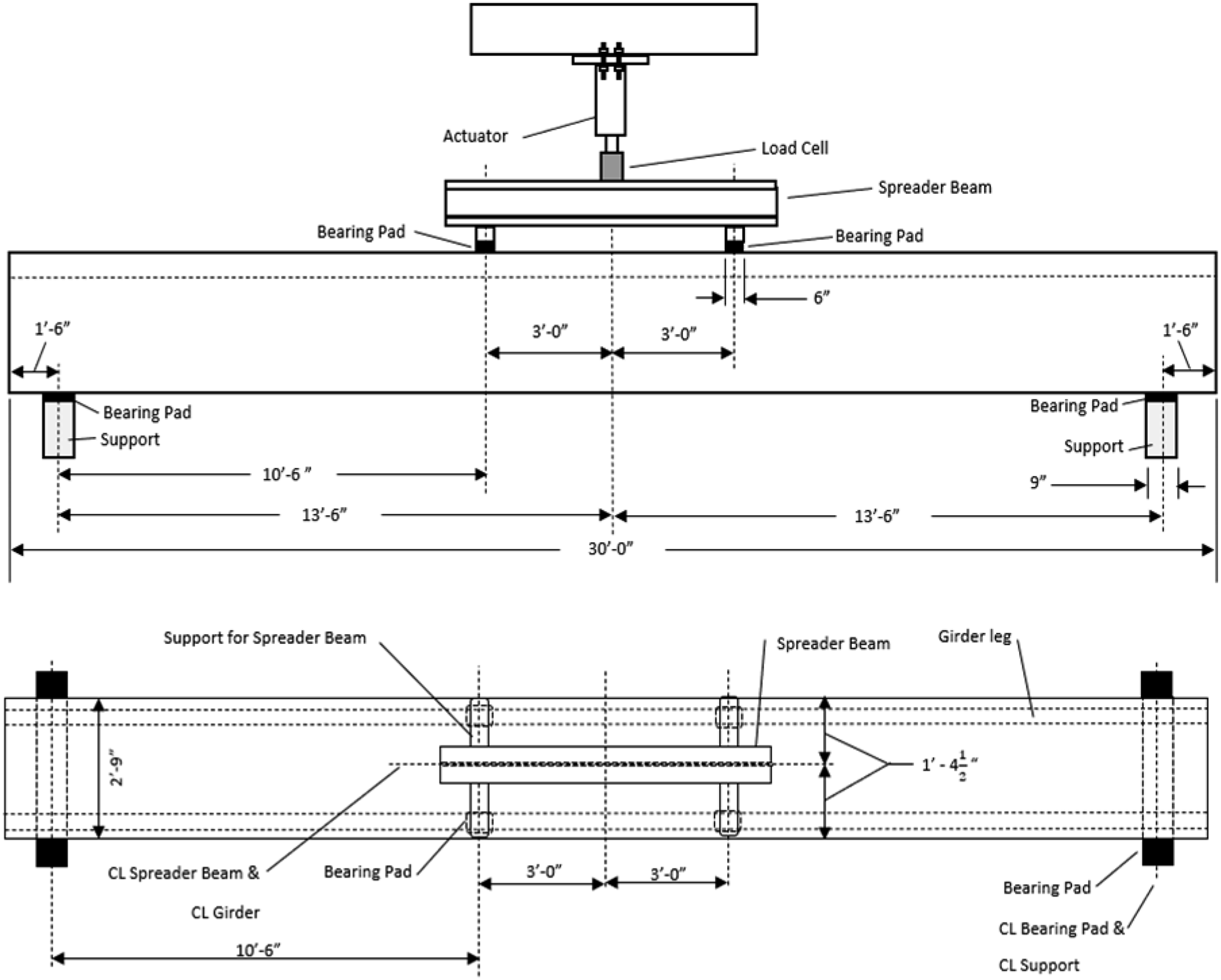

Potentiometric displacement transducers were utilized to quantify the vertical deflections at the quarter-span and mid-span locations of the girders. The application of the load was facilitated through a hydraulic actuator. To track the applied load magnitudes throughout the testing phase, both a calibrated load cell and a pressure gauge were employed, with the load cell having a maximum capacity of 250 kips. Data acquisition was conducted using a 32-channel system, which captured and logged the data in real time during the load application. Figure 3 provides visual documentation of the experimental configuration.

Figure 3.

Photographs of the test setup of the girders.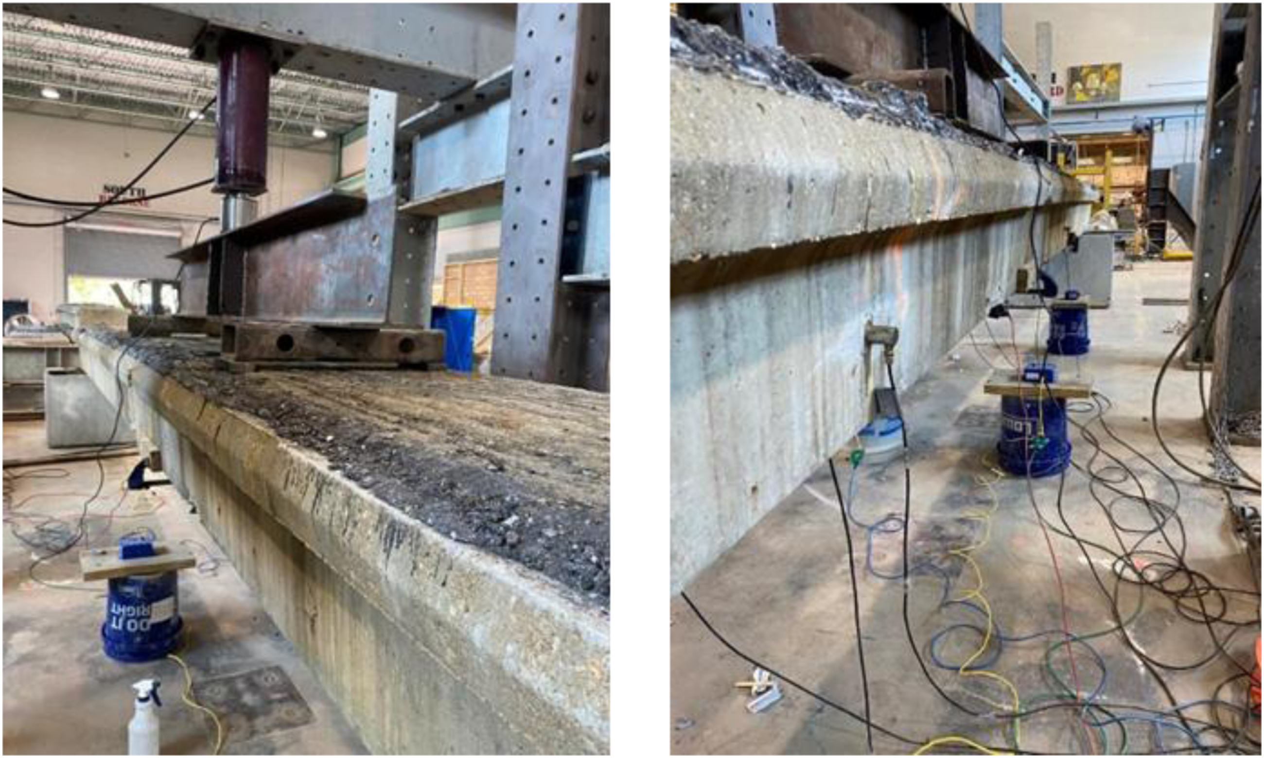

The loading protocol for the girders involved incremental cyclic loading, designed to replicate the dynamic effects of vehicular wheel loads on bridge girders. The initial load applied was one kip. Subsequently, the load was increased to four kips, sustained at this level for a duration of 60 s, and then reduced back to one kip, a sequence designated as load step 1 (L1). Following this, the load was escalated to eight kips, held steady for 60 s, and then decreased back to one kip, a process identified as load step 2 (L2). The sequence continued with the girders being subjected to a load of 12 kips, maintained for 60 s, and then diminished back to 1-kip, termed load step 3 (L3). The pattern persisted with an increment to 16 kips, upheld for 60 s, followed by a reduction to one kip, noted as load step 4 (L4). Finally, the girders experienced a load of 20 kips, again held for 60 s, before returning to one kip, referred to as load step 5 (L5). These load steps, from L1 to L5, were strategically structured to emulate the spectrum of vehicle loads anticipated during the service life of the girders. Figure 4 delineates the relationship between load and time for the tests.

Figure 4.

Load versus time.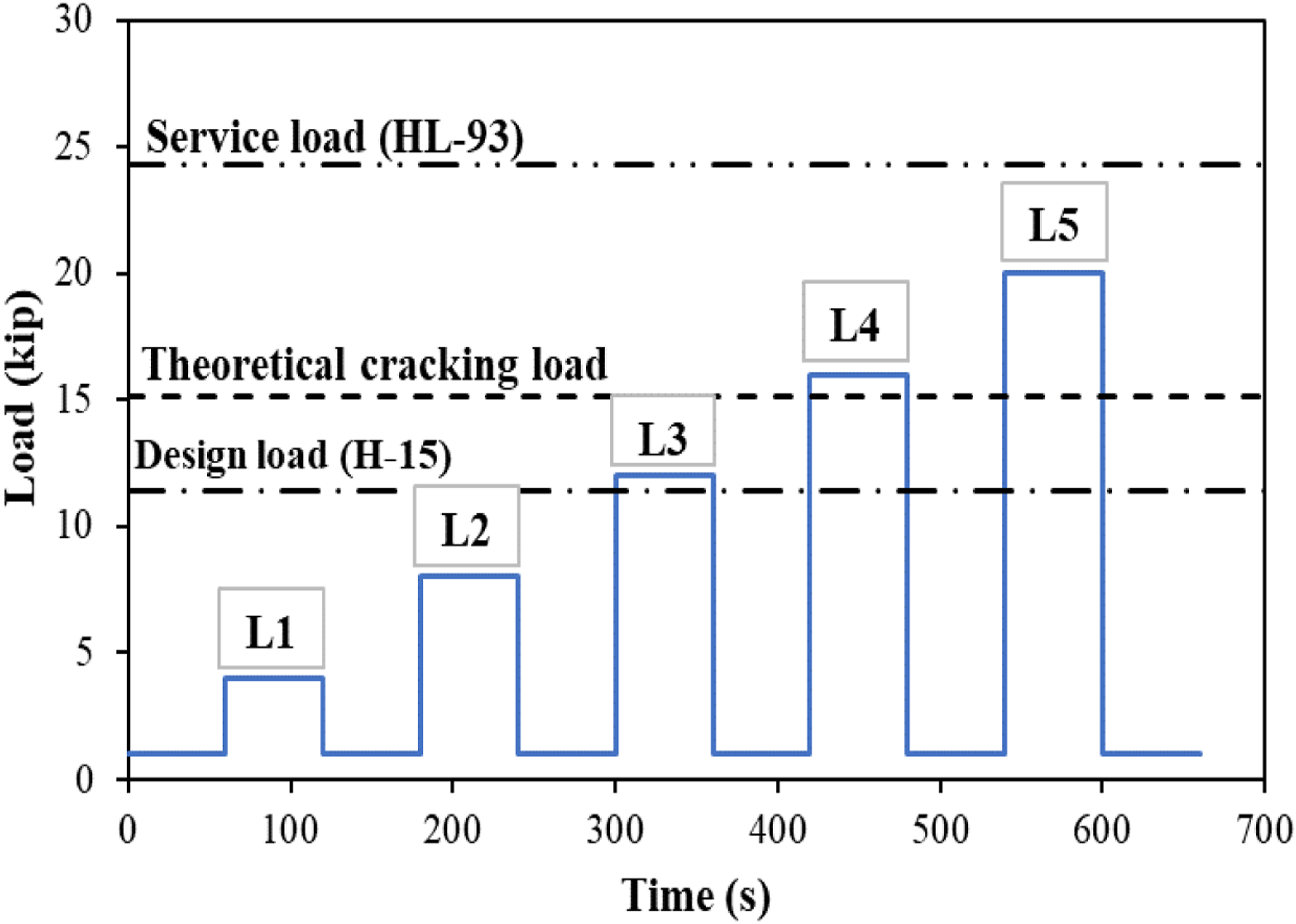

Acoustic emission

AE refers to the transient elastic waves propagated through a material when localized strain energy is rapidly released. AE sensors can capture high-frequency waves that emanate from the swift liberation of energy, typically associated with phenomena such as the expansion of cracks. An individual AE event captured by the sensors is termed a “hit”. Several features including amplitude, duration, rise time, energy, average frequency, and signal strength, as depicted in Figure 5, can be extracted from one hit.

Figure 5.

Schematic of acoustic emission parameters (Mohamed K ElBatanouny et al., 2014b).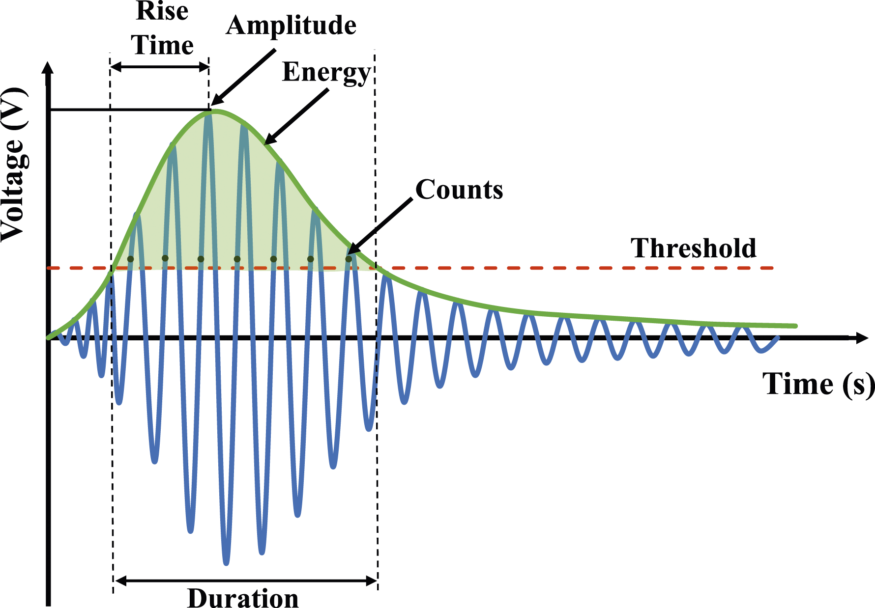

AE was recorded using the Sensor Highway II system, in conjunction with eight AE sensors. The sensors were differentiated into two categories: four of the broadband WDI type and four of the R6i resonance type, functioning within frequency ranges of 100-900 kHz and 40-100 kHz, respectively. Prior to the affixation of the sensors using double-bubble epoxy, the surfaces of the test specimens were meticulously cleaned. The sensors were arrayed on the specimen in a calculated manner to optimize the detection of AE phenomena and were integrated into the data acquisition system. Figure 6 illustrates the layout of the AE sensors. In alignment with ASTM E1316, pencil lead break was employed to evaluate the attenuation characteristics for each sensor. Throughout the testing, the threshold for detection was standardized at 50 dB across all channels, a level selected to suppress ambient noise yet maintain adequate sensitivity for the capture and documentation of AE occurrences.

Figure 6.

Elevation (top) and plan (bottom) instrumentation layout.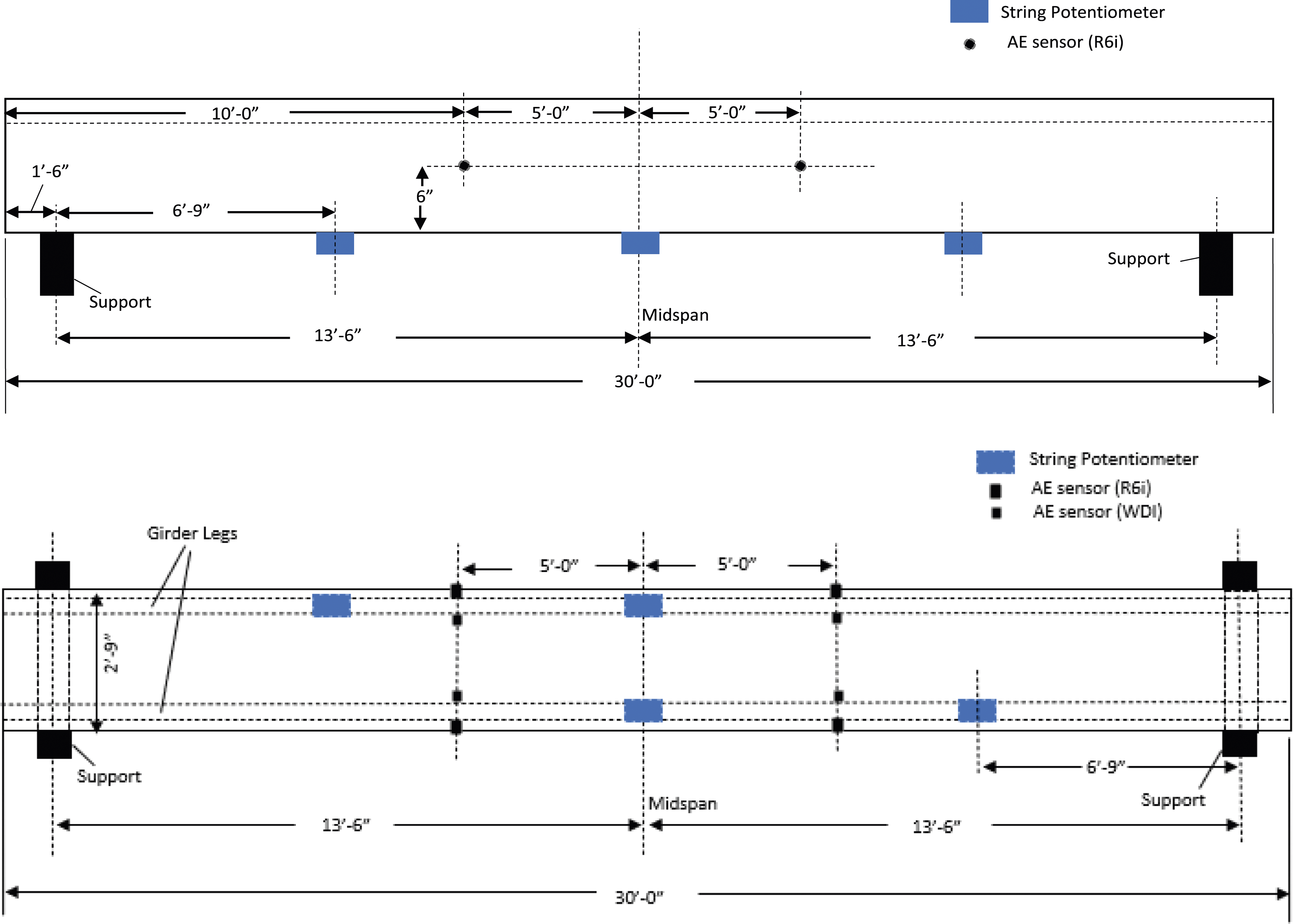

Data processing and methodology

Framework

AE signals were recorded during the tests for further analysis. Table 2 presents the AE parameters and their definitions that were employed in this study. Three machine learning algorithms are used in this study to classify a group of AE hits to their corresponding load steps based on their corresponding AE parameters. The rationale behind this method is that the variances among the 15 AE parameters would enable the machine learning algorithm to classify the data points. In field applications, the AE data collected from a vehicle passing over a bridge will be a group of AE hits, not a single AE hit. Hence, the overall goal was to classify a group of AE hits to their corresponding load step.

Table 2.

AE Signal Parameters.

Number	AE parameters	Definitions
1	Amplitude (dB)	The maximum amplitude at the peak of the wave
2	Count	The number of threshold crossings
3	Rise time (μs)	The time interval between the first threshold crossing and the maximum amplitude
4	Duration (μs)	The time between the first and last threshold crossing of signal
5	Average frequency (kHz)	Counts/Duration
6	Root mean square (RMS) (V)	The effective voltage with a characteristic time T_RMS for average ranging from 10 to 1000 ms
7	Average signal level (ASL) (V)	The effective voltage with a characteristic time T_ASL for average ranging from 10 to 1000 ms
8	Energy (10⁻¹⁴ V²s)	The measure of the electrical energy measured for an AE signal
9	Absolute energy	The absolute measure of the electrical energy measured for an AE signal
10	Reverberation frequency (kHz)	Frequency after the peak
11	Initial frequency (kHz)	Frequency before the peak
12	Signal strength	A parameter to evaluate the AE source strength
13	Counts to peak (PCNTS)	The number of threshold crossings from the first threshold crossing to the peak
14	Peak frequency (P-FRQ) (Hz)	Frequency of maximum signal contribution
15	Frequency centroid (C-FRQ) (Hz)	A parameter to characterize the overall frequency content of an AE signal

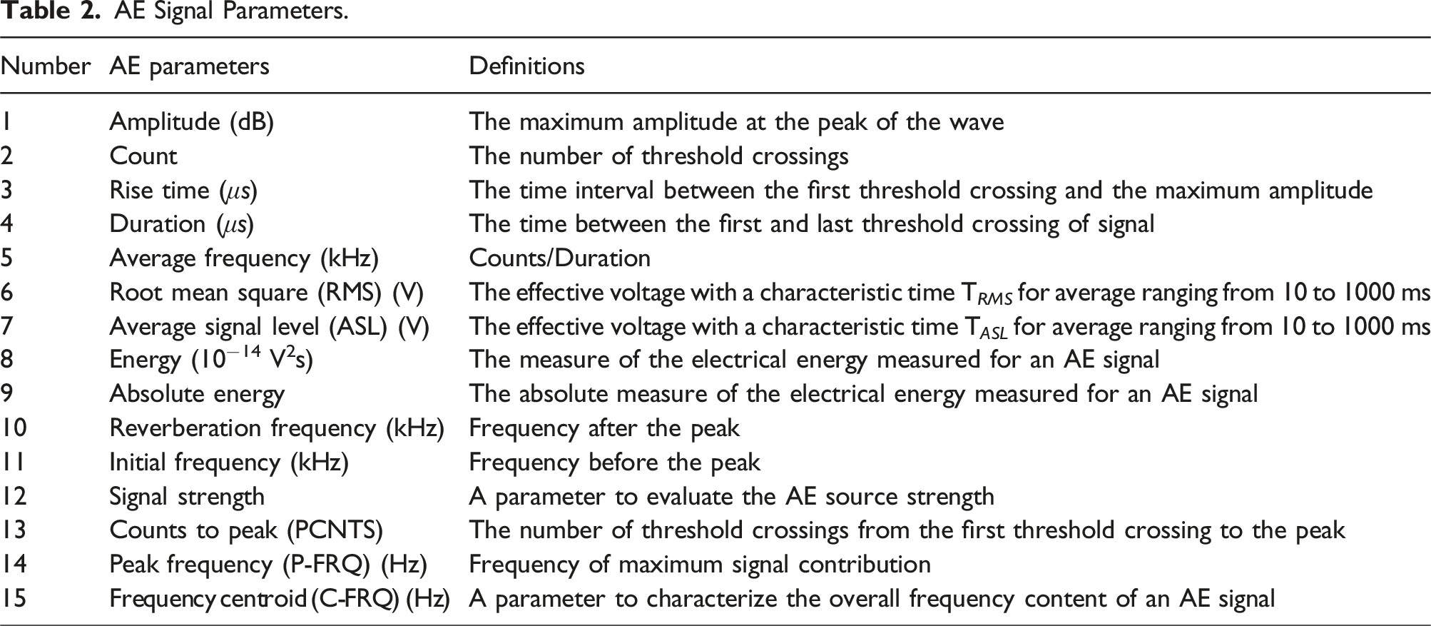
During the bending tests, AE signals were captured for subsequent examination. The AE parameters used in this paper and their respective definitions are summarized in Table 2. This paper leverages three distinct machine learning algorithms to categorize clusters of AE hits into their respective load steps based on the AE parameters associated with each hit. The underlying assumption of this approach is that the differences across the 15 AE parameters would provide the machine learning models with sufficient discriminatory power to sort the data points accurately. In practical scenarios, such as monitoring vehicular traffic over a bridge, the AE data acquired would consist of a collection of AE hits rather than isolated hit. Therefore, the primary objective is to correctly assign a batch of AE hits to the specific load step they represent.

The data collected for one girder (T1) was used to assess the performance of the three machine learning algorithms. The total data collected from the test was 30,274 hits. The girder was loaded stepwise cyclic (five load steps: L1, L2, L3, L4, and L5). During the initial loading phase, designated as L1, a total of 241 Acoustic Emission (AE) hits were recorded. Subsequent loading phases, specifically L2 through L5, yielded a progressive increase in AE hits, with counts of 1395, 5337, 8140, and 15,161, respectively. Due to the limited dataset obtained from L1, the AE hits classification was confined to data procured from L2 to L5. Figure 7 illustrates the distribution of AE hits across the various loading stages for the examination conducted.

Figure 7.

Amplitude and load versus time for the test.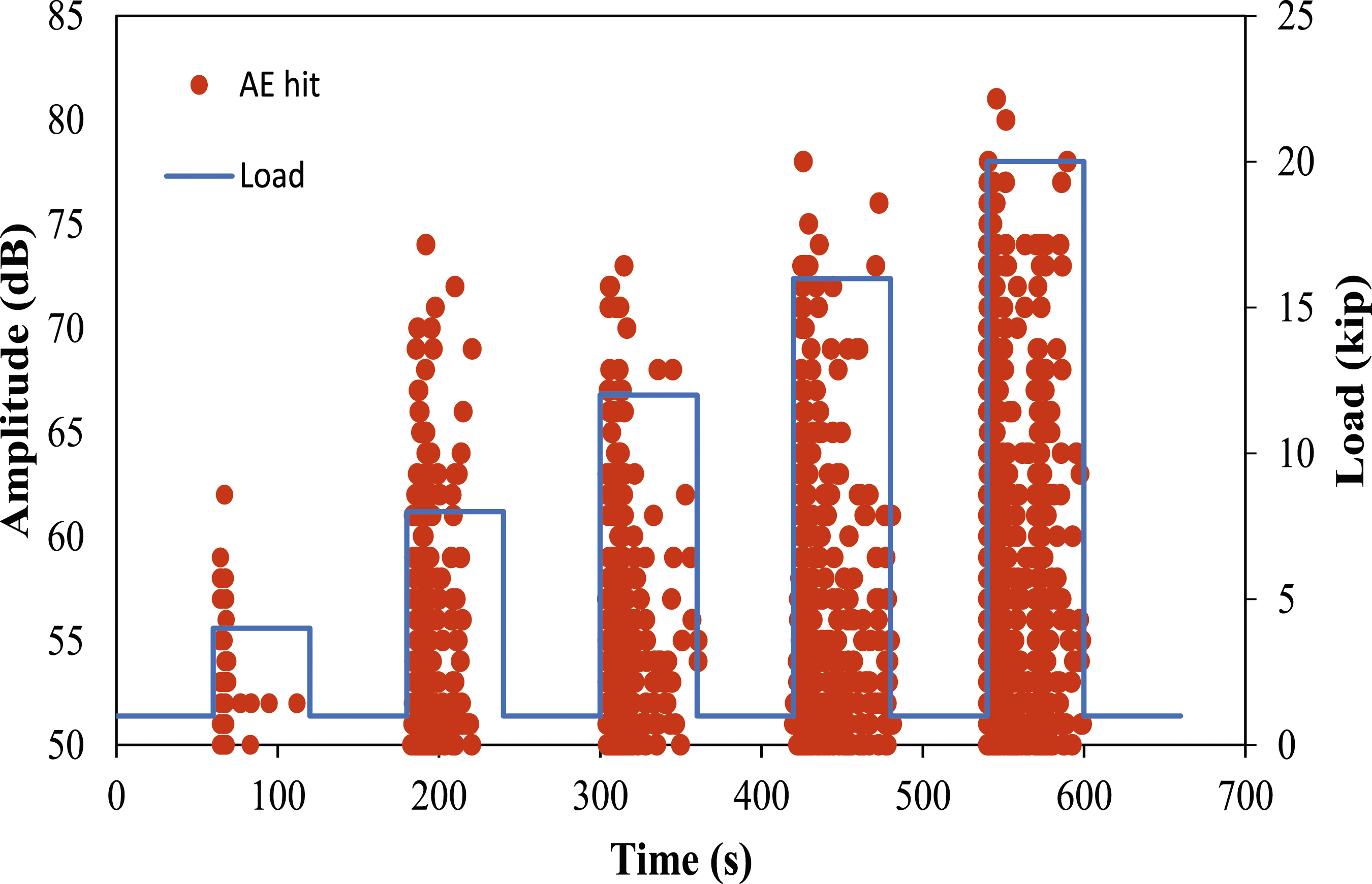

The machine learning model goes through three phases of classification: training, validation, and testing. Most of the AE hits in the total dataset from the test come from L5 (15,161 hits out of 30,274 hits), which causes an imbalance issue in the machine learning model as reported in the findings of (Laxman et al., 2023). To address the imbalance issue, a method named balanced training was proposed, which ensures that an equal amount of data from each load step is fed into each model. It was determined that the ratio of the number of hits belonging to L3 (5,137 hits), L4 (7,940 hits), and L5 (14,961 hits) to L2 (1,195 hits) was 4 to 1, six to 1, and 12 to 1, respectively. To even out the data, a total of 288 data combinations ( $C_{4}^{1} \times C_{6}^{1} \times C_{12}^{1}$ ) were composed to balance the data. Using these combinations as training data, 288 different models were trained and validated. Each machine learning model was fed with the total data from L2 (1,195 hits) and a random dataset (1,195 hits) from L3, L4, and L5, respectively. Hence, each model had an equal amount of data (1,195 hits) from each load step. This procedure is referred to as balanced training (BT). A group of AE hits consisting of 200 hits from each load step (L2, L3, L4, and L5) was collected prior to training and validation. The testing data collected was used to evaluate these models. Each model contributed a vote towards the classification, with the collective decision being determined by the principle of majority rule among the model votes. Figure 8 shows the process of the framework.

Figure 8.

Balanced training (BT) and testing for the machine learning models.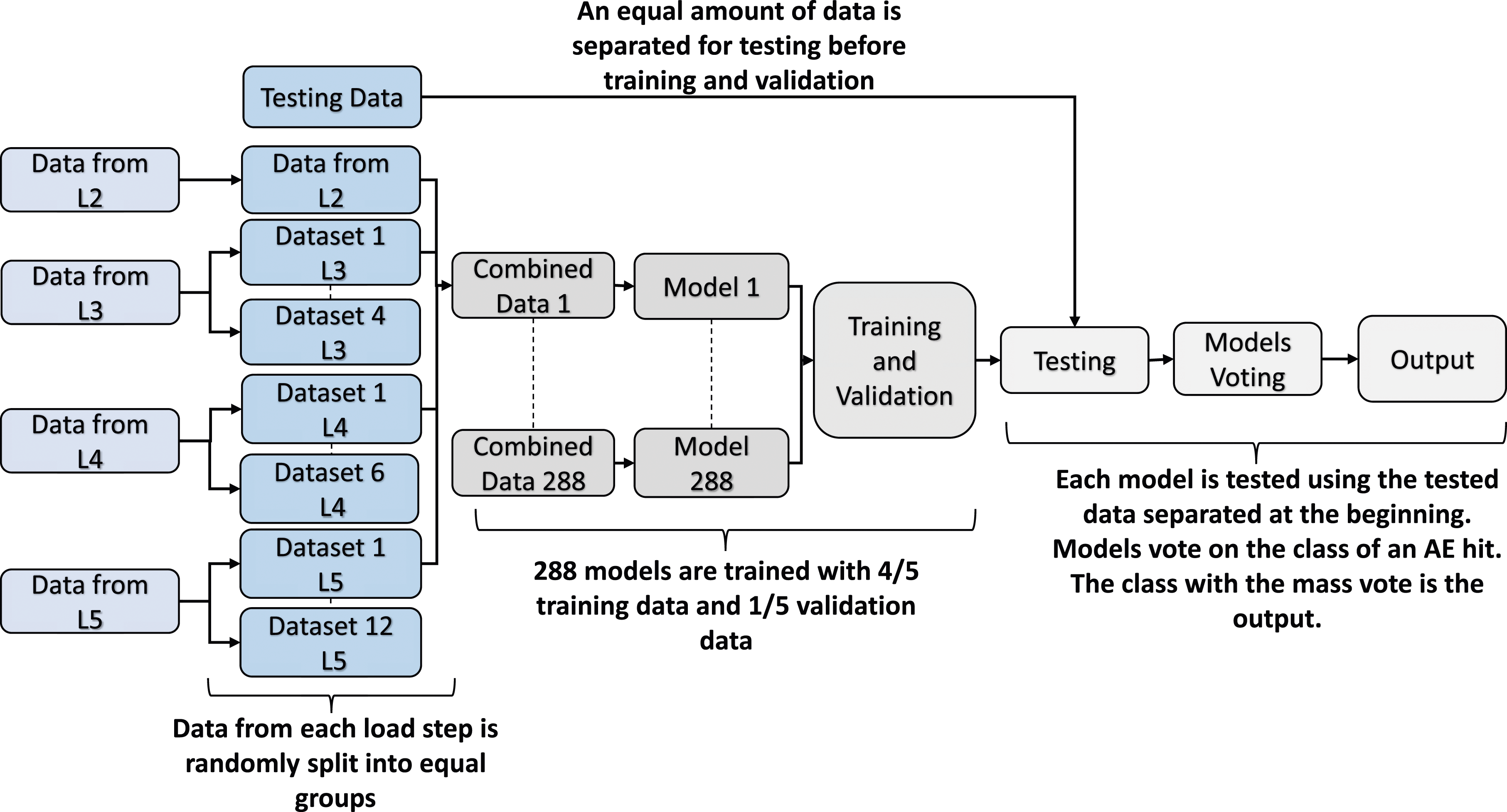

It should be noted that if an AE hit is entered into the BT model shown in Figure 8, the predicted result is the load step to which this single AE hit belongs. However, the AE hits accrued from vehicular loading will manifest as a group of AE hits, as depicted in Figure 9, rather than an isolated AE hit. If all AE hits are entered into the BT model, a set of predicted loads will be obtained. Therefore, a decision-making process was developed in this application to finally determine the load step. As shown in Figure 9, the AE hits generated by the load step were assigned to the trained BT machine learning model. Then, the output was converted into the probabilities that this load belongs to the steps. The final determination was made based on the maximum probability.

Figure 9.

Decision-making process.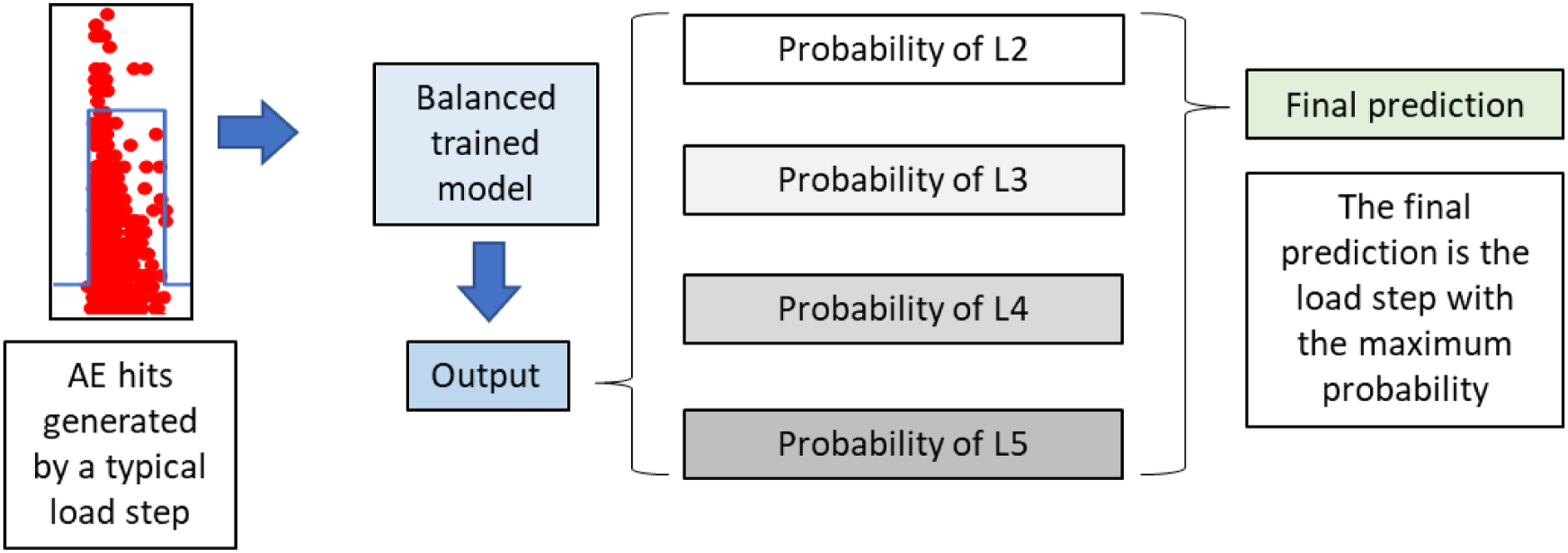

The Artificial Neural Networks (ANN), AdaBoost, and random forest algorithms improved by the BT strategy were used in this study to categorize the group of AE hits according to the vehicle loads they corresponded to, utilizing the respective AE parameters.

Artificial neural network

The study utilized a backpropagation artificial neural network (BP-ANN), a prevalent technique within the domain of ANN methodologies as referenced in literature (Hecht-Nielsen, 1992). This network architecture is constructed with an input layer, several hidden layers, and an output layer (Jian-Zhou Wang et al., 2011). Each of these layers contains a multitude of processing units termed neurons. Moreover, these neurons are interconnected with all other neurons in the adjacent layers, forming a complex network (Tsai and Lee, 1999). The quantity of neurons present in the input and output layers is directly proportional to the number of input features and the dimensionality of the output, respectively (Erb, 1993).

Figure 10 depicts a typical three-layer artificial neural network comprised of layers i, j, and k. The number of neurons is a for layer i, b for layer j, and c for layer k. The weights between neurons in neighboring layers are denoted by W(ij) and W(kj). The values of a and c are related to the problem for solving, whereas the network designer determines b. Two hidden layers with 15 neurons were employed in this study.

Figure 10.

Three-layer artificial neural network.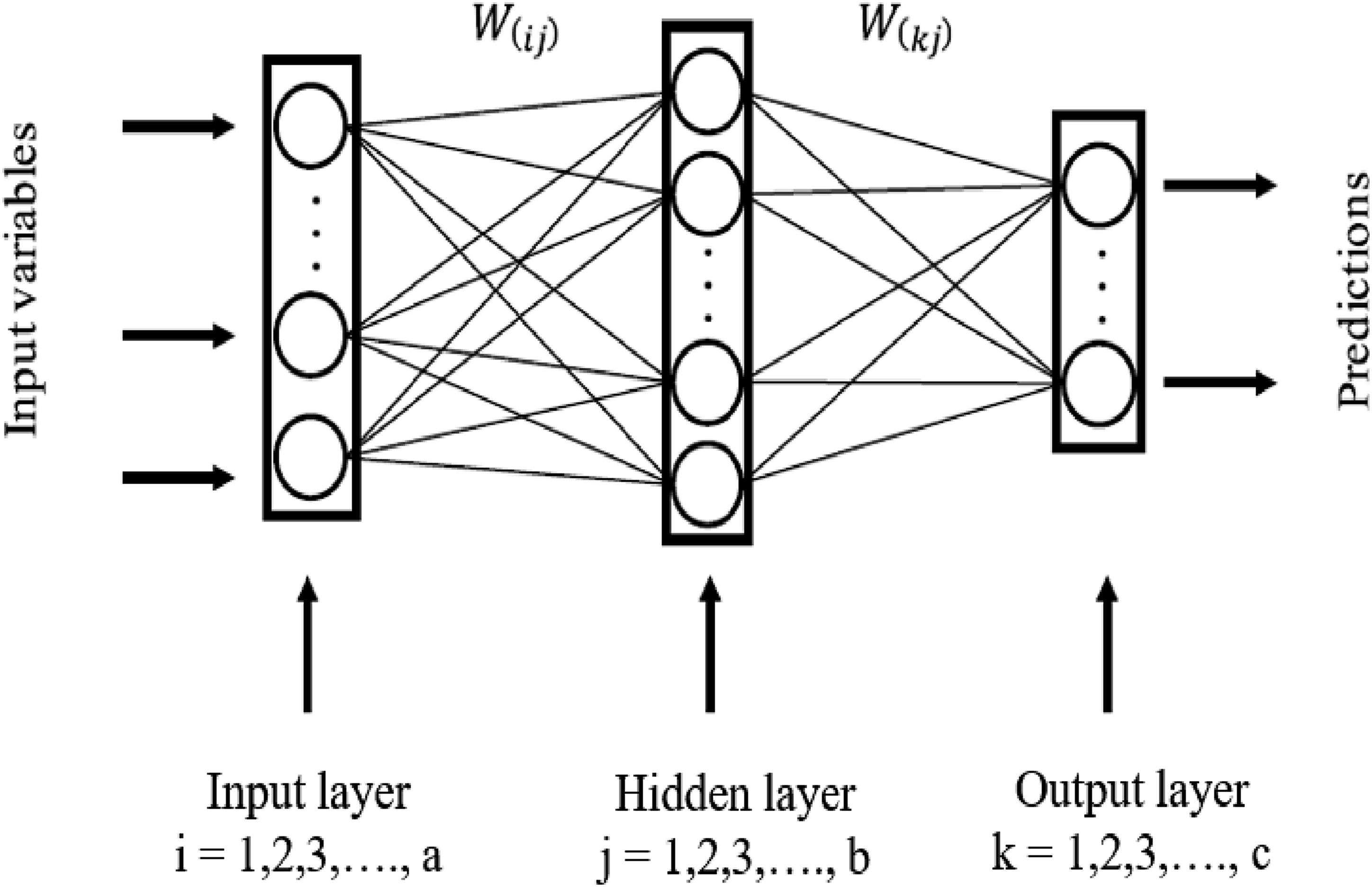

A BP network is calculated using feedforward and error-backward computations. In feedforward computations, the input layer neurons receive the processed data, and equation (1) calculates the weighted sum corresponding to each neuron in the subsequent layer.

{n e t}_{(i)} = \sum_{j = 1}^{n} W_{(i j)} \cdot O_{(j)}

(1)

Where net is the net input of the i-th neuron,

W_{(i j)}

is the weight, and

O_{(j)}

is the output of the neuron.

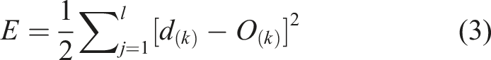
The weighted sum is submitted to the activation function, which may be linear, nonlinear, or a unit step function, to determine the output of the i-th neuron. The S-type activation function is represented in equation (2), which is typically used to explain the nonlinearity of the system. The result obtained by the output layer will be employed to generate an error. Error E is calculated as shown in equation (3).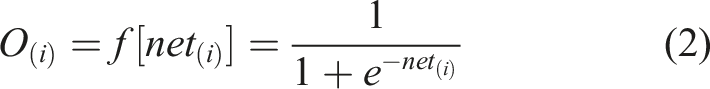

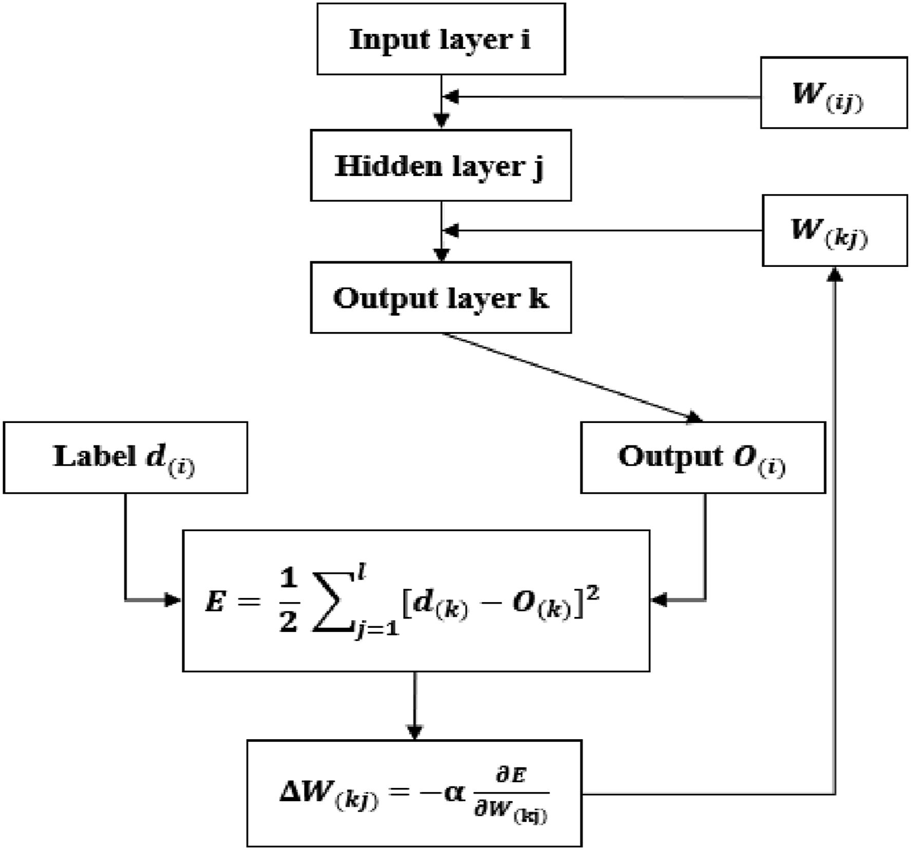
O_{(i)} = f [{n e t}_{(i)}] = \frac{1}{1 + e^{{- n e t}_{(i)}}}

(2)

E = \frac{1}{2} \sum_{j = 1}^{l} {[d_{(k)} - O_{(k)}]}^{2}

(3)

Where,

d_{(k)}

is the label value.

O_{(k)}

is the prediction value in the k-th neuron of the output layer.

The error of the output layer will be backpropagated to the previous adjacent layer using the gradient descent method, and lastly propagated to the input layer to produce more accurate results. Equation (4) yields the value of the weight change. All connection weights are initially assigned random values and subsequently changed based on the outcomes of the BP training process. Figure 11 depicts the mechanism of a backpropagation network.

Δ W_{(k j)} = - α \frac{\partial E}{{\partial W}_{(kj)}}

(4)

Where

α

is the learning rate that adjusts the amplitude of the weight change.

Figure 11.

Mechanism of a backpropagation network.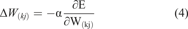

AdaBoost

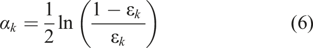
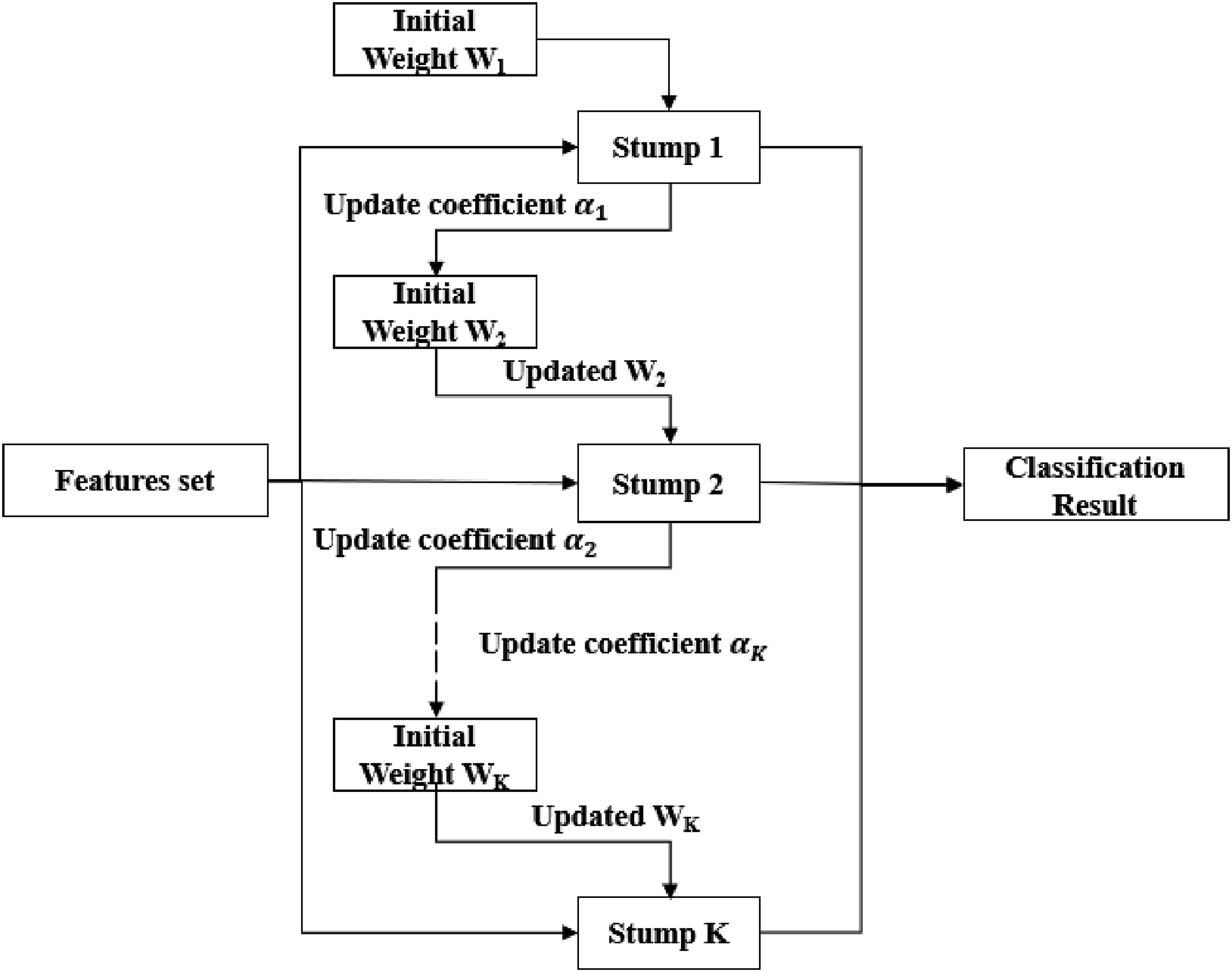
The Boosting algorithm is an integrated learning method that can improve multiple weak learning models (Rätsch et al., 2001). “Adaptive Boosting” is referred to as AdaBoost. In contrast to the random forest, the weak learning model utilized in the AdaBoost algorithm is usually just a decision node and two leaf nodes referred to as a decision stump (referred to as a stump hereafter). The stump can only use one variable to decide. AdaBoost is adaptive in that succeeding stumps are weighted in favor of instances misclassified by prior stumps. Each stump inside the AdaBoost obtains a function through multiple iterations. At the end of the iterations, each stump is assigned a weight. The final classification is voted from the results of all the stumps, considering the weight. In other words, some stumps get more say in the classification than others (Schapire, 2013).

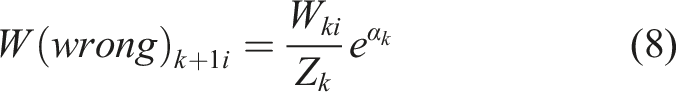
An initial weight set (W) is assigned to the AdaBoost model: W = ( $W_{1}$ , $W_{2}$ , …, $W_{N}$ ). Every element in the weight set has the same initial weight of 1/N. Assuming the AdaBoost model has k stumps. Equation (5) can calculate the kth stump, and the updated coefficient of the weight can be obtained by equation (6).

ε_{k} = \sum_{i = 1}^{N} W_{k i}, T_{k} (X_{i}) \neq y_{i}

(5)

α_{k} = \frac{1}{2} \ln (\frac{1 - ε_{k}}{ε_{k}})

(6)

The updated weight $W_{k + 1}$ for the next stump $T_{k + 1}$ can be provided by Equation (7) and Equation (8):

W {(c o r r e c t)}_{k + 1 i} = \frac{W_{k i}}{Z_{k}} e^{{- α}_{k}}

(7)

W {(w r o n g)}_{k + 1 i} = \frac{W_{k i}}{Z_{k}} e^{α_{k}}

(8)

Z_{k} = sum (W_{k})

(9)

Where W (correct) refers to the weight assigned to the input data correctly classified by the last stump and W (wrong) refers to the weight assigned to the input data incorrectly classified by the last stump.

Z_{k}

is the normalization factor. The architecture of the AdaBoost algorithm is shown in Figure 12. The number of stumps employed in this study was one hundred.

Figure 12.

The architecture of the AdaBoost algorithm.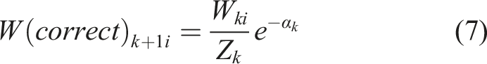

Random forest

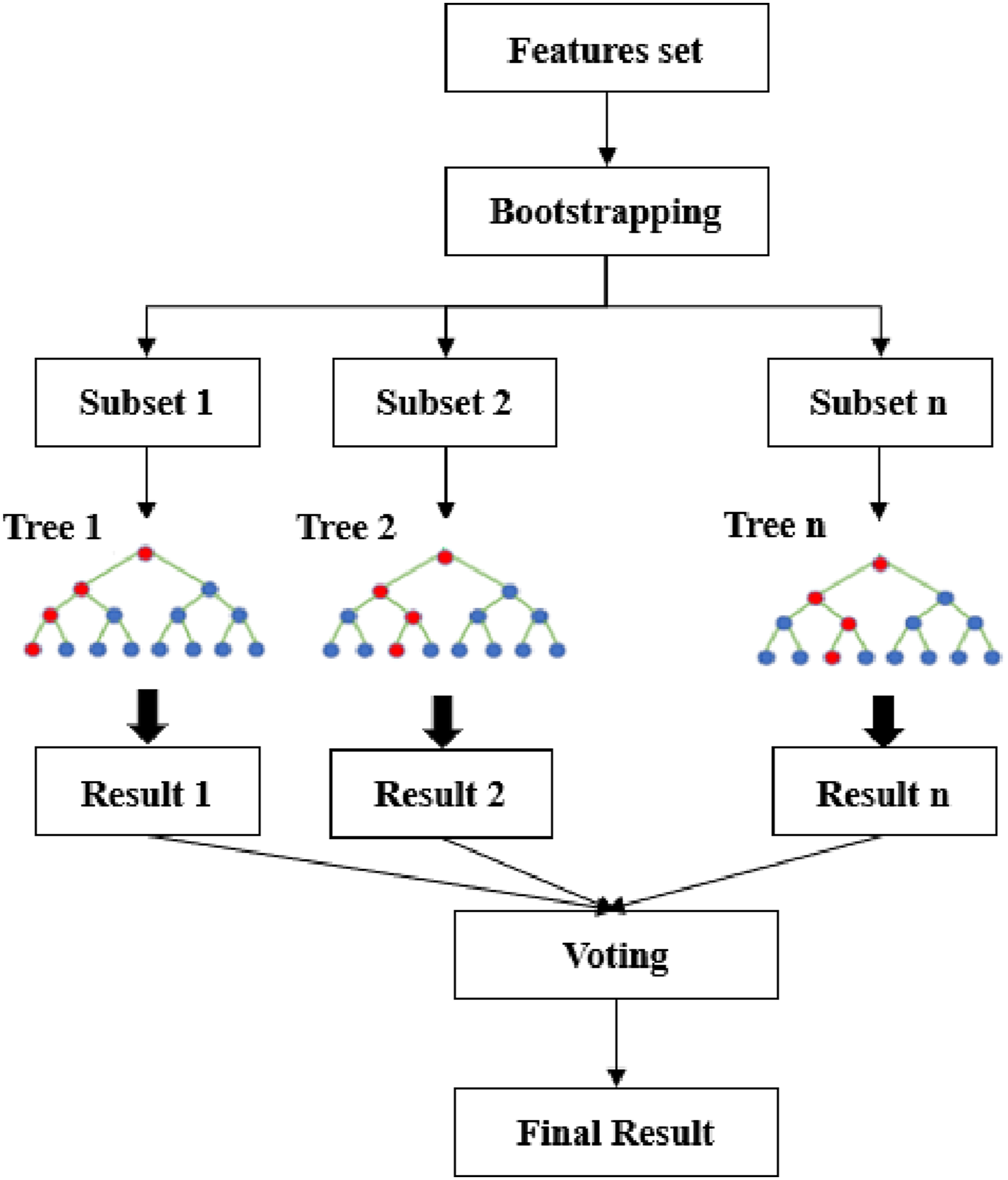
The random forest algorithm operates as an ensemble learning method, specifically utilizing bagging (Breiman, 2001). It integrates several base learners, which are typically of weaker predictive capability. The final prediction of the ensemble is derived from aggregating the predictions of these base learners through voting or averaging (Sandri and Zuccolotto, 2006). A base learner, in this context, is characterized as a model whose accuracy is only slightly better than random chance. Within the framework of a random forest, decision trees serve as these base learners. In the structure of a decision tree, a dataset is categorized using a variety of attributes. Nodes within the tree are of two types: decision nodes, which implement a condition to divide the data, and leaf nodes, which assign the class label. Each node in the tree evaluates a condition that determines how to branch out to the next decision node, based on the efficacy of the attributes at that point. As the data traverses through the successive layers of decision nodes, the classes within the samples become more homogenous. The classification outcome of the decision tree is determined at the leaf nodes, which signify the result of the data segmentation process.

The Gini impurity of the node is employed as the branching criteria in this study for generating the decision tree. The Gini impurity of a node refers to the probability that the sample was incorrectly classified and is obtained by equation (10). If the Gini impurity is less than a predetermined threshold (typically zero), it indicates that the samples belong to the same class. Otherwise, the sample is split into two parts, N1 and N2, as given in equation (11), and then assigned to two sub-nodes. Figure 13 shows the architecture of the random forest. The number of decision trees employed in this study was one hundred.

Gini (N) = 1 - \sum_{i = 1}^{k} P (\frac{i}{t})

(10)

Where

P (\frac{i}{t})

is the probability of category i at node t.

Gini (N, F) = \frac{N 1}{N} Gini (N 1) + \frac{N 2}{N} Gini (N 2)

(11)

Figure 13.

The architecture of the random forest.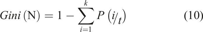

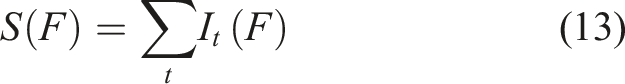
The random forest model can determine and assess the significance of features through the feature division process while classifying. The method is shown in equations (12) and (13).

I_{t} (F) = G i n i | (N) - G i n i (N, F)

(12)

S (F) = \sum_{t} I_{t} (F)

(13)

Where

I_{t} (F)

refers to the decrease of the Gini impurity before and after node t is split into two sub-nodes according to feature F. The absolute importance of feature

S (F)

can be defined as the sum of

I_{t} (F)

at all nodes split by feature F.

Results and discussion

Three improved machine learning models were developed to classify a group of AE hits using 15 AE parameters. The collected AE data for a vehicle passing through a bridge in field applications will consist of a group of AE hits, rather than a single AE hit. Hence, the overall goal was to classify a group of AE hits to their corresponding load step.

Performance of BT-ANN

The ANN model was fed with data from the test (T1). AE hits were divided into four data sets, and labeled as L2, L3, L4, and L5. As input, these data sets were fed into the BT-ANN (balanced training ANN). Prior to training and validation, a randomly selected group of AE hits (200 hits) was taken from each data set for testing. To resolve the imbalance issue, a balanced training data set was developed where 288 different models were trained using even data from each load step. The ANN randomly selected 4/5 of the data for training and 1/5 of the data for validation. Then the models were tested, and each model voted. Most of the votes determined the classification of the AE hits.

The AE hits gathered from the vehicle loads will be a group of AE hits rather than a single AE hit. Therefore, the classification aimed to identify the corresponding load step for each group of AE hits (200 hits). First, a group of AE hits (200 hits) was classified into their corresponding load step based on the maximum number of AE hits assigned to each load step.

Figure 14 presents the outputs of the BT-ANN model and the decision-making process when the AE data generated by the vehicle loads are input to the model. For the data caused by L2, the number of AE hits correctly classified to L2 was 94, whereas 46, 21, and 39 were incorrectly classified to L3, L4, and L5, respectively. Since the largest number of hits were classified as L2 for this group of AE hits (200), it can be considered that the probability of the number of AE hits generated by L2 is the largest. Hence, this group of AE hits was classified correctly into L2.

Figure 14.

Output of BT-ANN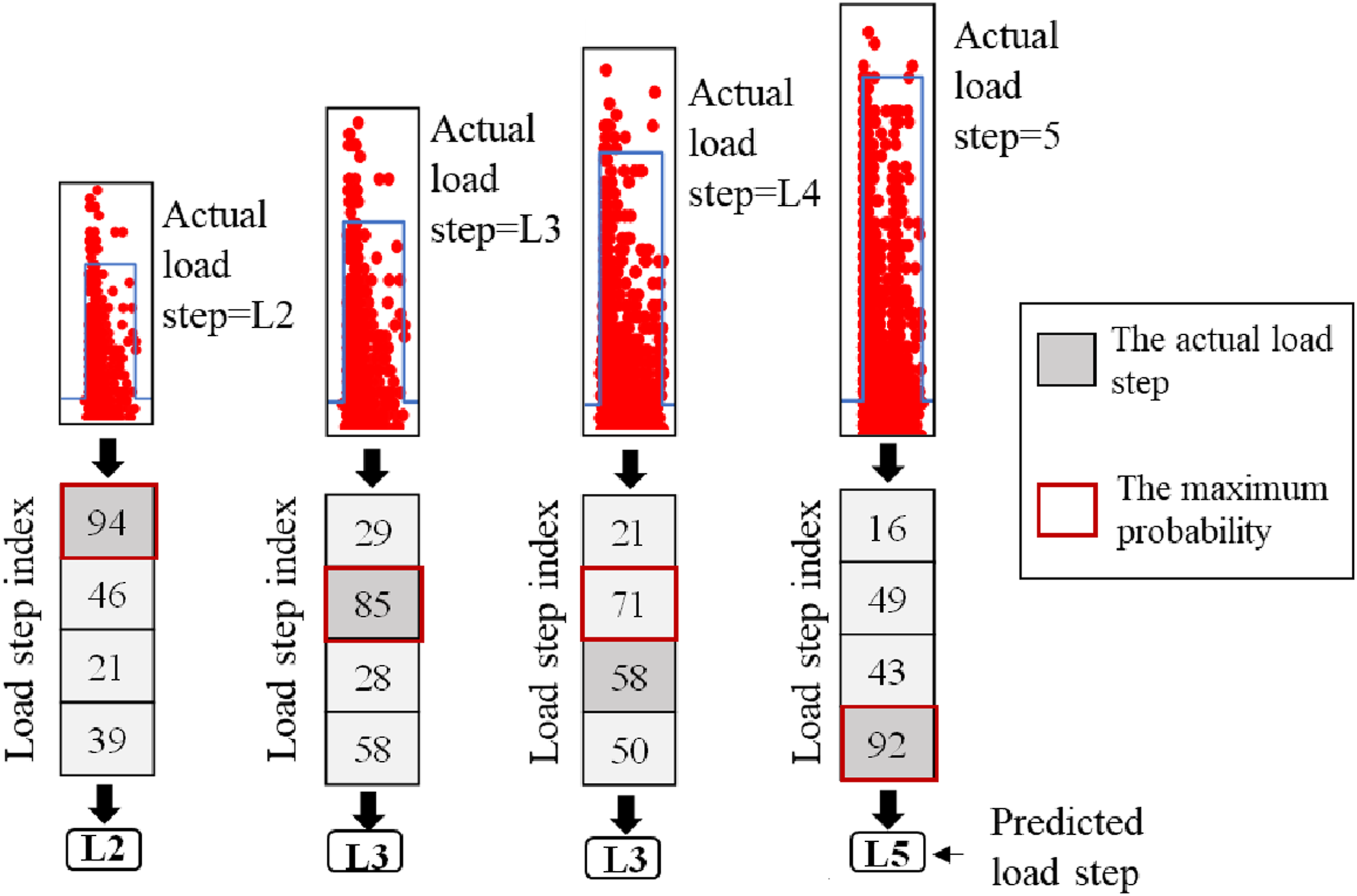

For the data generated by L3, the number of AE hits accurately assigned to L3 was 85, while 29, 28, and 58 were inaccurately assigned to L2, L4, and L5, respectively. It is obvious that the probability of those AE hits being generated by L3 is the largest in this grouping. Therefore, this group of AE hits (200) was classified accurately into L3. According to the above rules, the AE data generated by L4 is incorrectly classified as L3. The data from L5 is correctly classified as L5. The results show that, except for misclassifying L4 as L3, the BT-ANN model correctly classifies each group of AE hits to its corresponding load step.

In addition, a scenario was developed to eliminate the randomness in the data selection and determine the model’s overall accuracy. One hundred groups of AE hits were randomly selected, and the data was tested on the trained model (BT-ANN). This scenario was named GTANN (Group Testing on ANN). The final classification (Figure 17(a)) presents the quantity of groups of AE hits that were assigned to their corresponding load step.

Performance of BT-AdaBoost

Similarly, the AdaBoost model was fed with data from the test (T1). AE hits were separated into four data sets and labeled as L2, L3, L4, and L5. These data sets were the input for the BT-AdaBoost (balanced training AdaBoost). Before training and validation, a group of AE hits (200 hits) was randomly selected from each data set for testing. Even data from each load step was used to train 288 different models to address the imbalance issue. The AdaBoost model randomly selected 4/5 and 1/5 of the data for training and validation, respectively. Next, the models were tested, and each model cast a vote. AE hits were classified based on the majority of the votes.

Following the procedure mentioned in section 4.1, the first step was to allocate a group of 200 AE hits to their associated load step based on the maximum number of AE hits allotted to each load step. Figure 15 shows the outputs of the BT-AdaBoost model and the decision-making process when the AE caused by the vehicle loads is input to the model. For the data generated by L2, the number of AE hits correctly assigned to L2 was 92, while 19, 43, and 46 were incorrectly assigned to L3, L4, and L5, respectively. The majority of the AE hits were assigned to L2, showing the highest probability of this group of AE hits was correctly correlated to L2. Following the above rules, the AE data caused by L3 and L4 were incorrectly assigned to L5. The data from L5 was correctly assigned to L5. The results indicate that the BT-AdaBoost model correctly classified the group of AE hits belonging to L2 and L5 to their corresponding load step. However, the group of AE hits belonging to L3 and L4 were misclassified to L5.

Figure 15.

Output of BT-AdaBoost.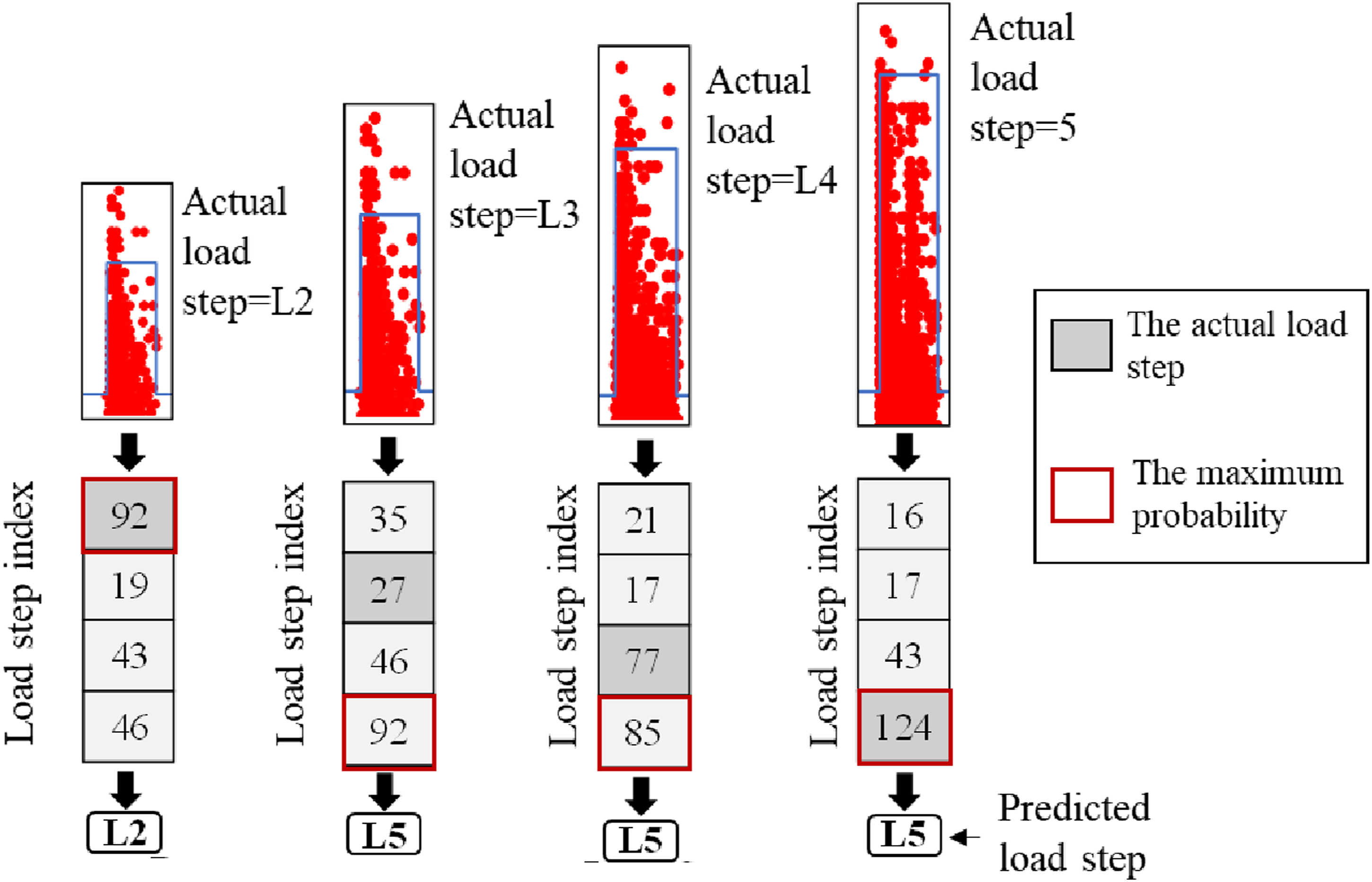

Moreover, a scenario was created to reduce the randomization in data selection and assess the overall reliability of the model. One hundred random samples of group AE hits were chosen, and the data was evaluated on the trained model (BT-AdaBoost). This scenario was called GTAdaBoost (Group Testing on AdaBoost). Figure 17(b) shows the final classification of these groups of AE hits that were allocated to their respective load steps.

Performance of BT-RF

A random forest model was developed to compare the results of ANN and AdaBoost models. The data from the test (T1) was fed to the BT-RF (balanced training random forest). AE hits were split into four data sets and labeled as L2, L3, L4, and L5. A group of AE hits (200 hits) was randomly selected from each data set for testing prior to training and validation. An equal amount of data from each load step was utilized for training 288 different models to solve the imbalance issue. The random forest model used 4/5 of the data for training and 1/5 for validation. Next, the models were tested, and each model voted on the class of AE hits. The majority of the votes rule was applied to obtain the final classification.

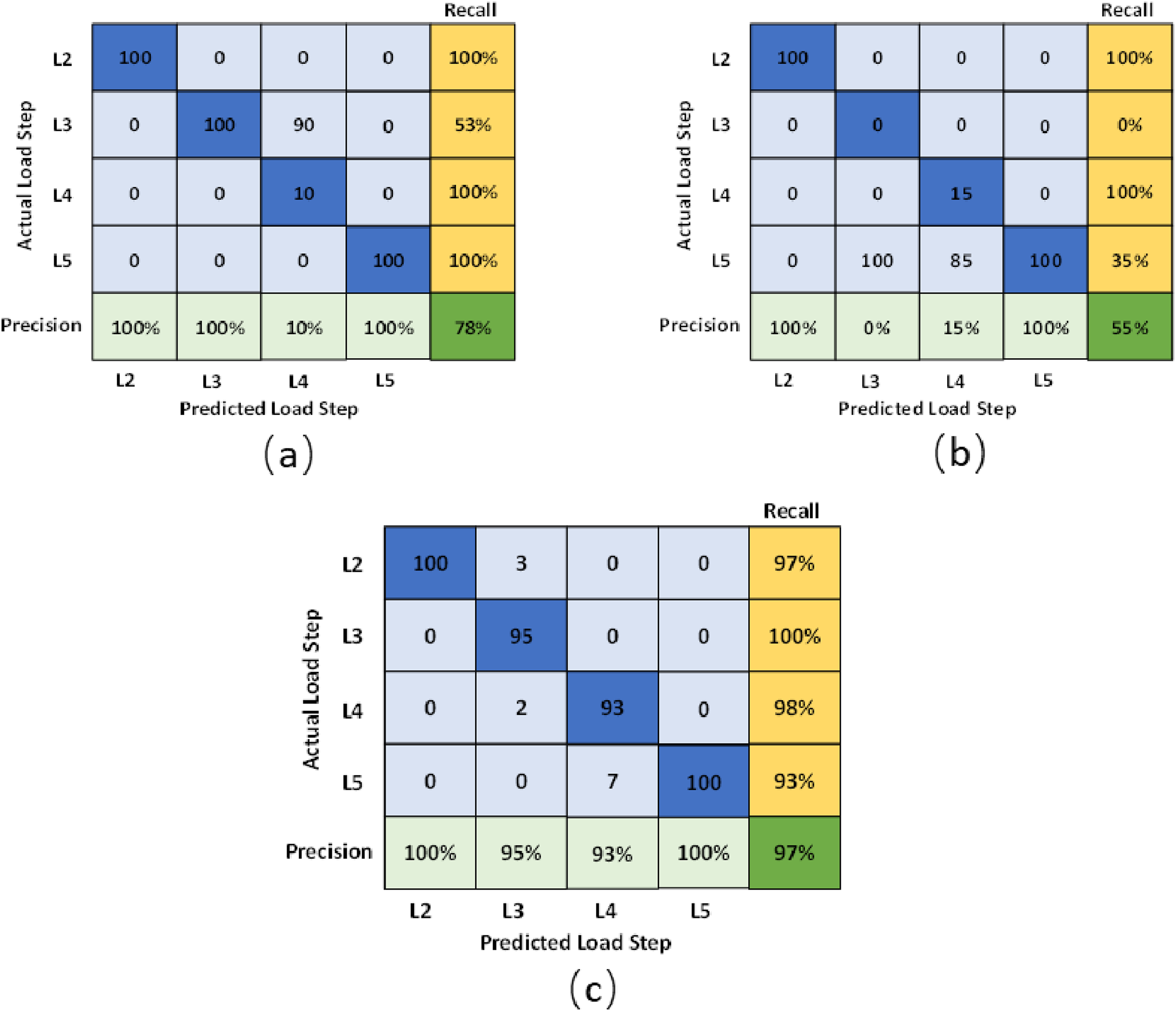
First, a group of AE hits (200 hits) was assigned to their corresponding load step according to the maximum number of hits classified to each load step. Figure 16 displays the results of the BT-RF and the decision-making process when the AE data produced by the applied loads are input into the model. For the data produced by L2, the number of AE hits accurately classified to L2 was 112, whereas 48, 21, and 19 were misclassified to L3, L4, and L5, respectively. Since the maximum number of AE hits was allocated to L2 for this group of AE hits, the probability of those AE hits being allocated to L2 is the highest. Thus, this group of AE hits was accurately classified as L2. Following the same decision-making process, the AE data generated by L3, L4, and L5 were correctly classified into L3, L4, and L5, respectively. The results show that the BT-RF model correctly classified each group of AE hits to their corresponding load step.

Figure 16.

Output of BT-random forest.

Figure 17.

The confusion matrixes of (a) GTANN; (b) GTAdaBoost; (c) GTRF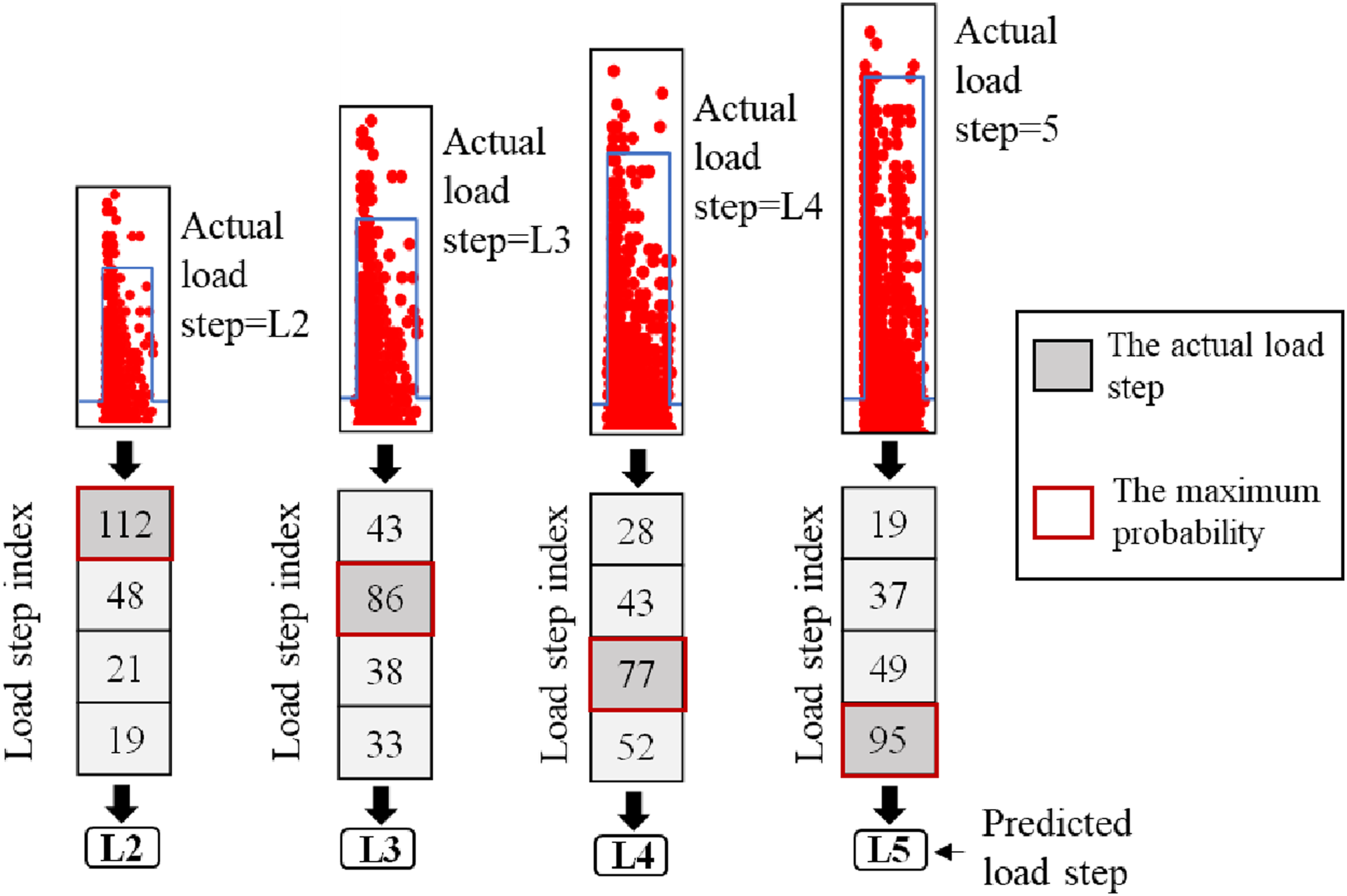

Furthermore, a scenario was designed to decrease randomness in data selection and evaluate the overall credibility of the model. One hundred groups of AE hits were randomly selected, and the data was assessed on the trained model (BT-RF). This scenario was named GTRF (Group Testing on random forest). The final classification in Figure 17(c) depicts how many of these 100 groups of AE hits were assigned to their related load step.

Comparison and discussion

A scenario was designed to assess the accuracy of the three improved machine learning models that were developed to classify a group of AE hits according to their respective load steps. The accuracy value is given by equation (14). The accuracies of the classification using three different machine learning algorithms are presented in Table 3. The approach using random forest (GT-RF) provides the highest accuracy 97%, whereas the accuracies by the ANN approach (GT-ANN) and the AdaBoost approach (GT-AdaBoost) are 78% and 55%, respectively.

A c c u r a c y = \frac{N u m b e r o f c o r r e c t l y c l a s s i f i e d g r o u p s o f A E h i t s i n t h e t e s t}{T o t a l n u m b e r o f g r o u p s o f A E h i t s i n t h e t e s t}

(14)

Table 3.

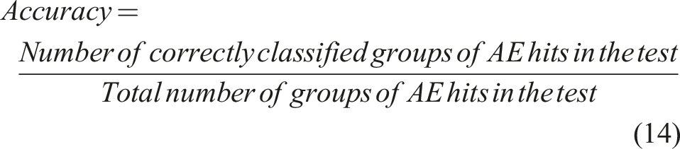
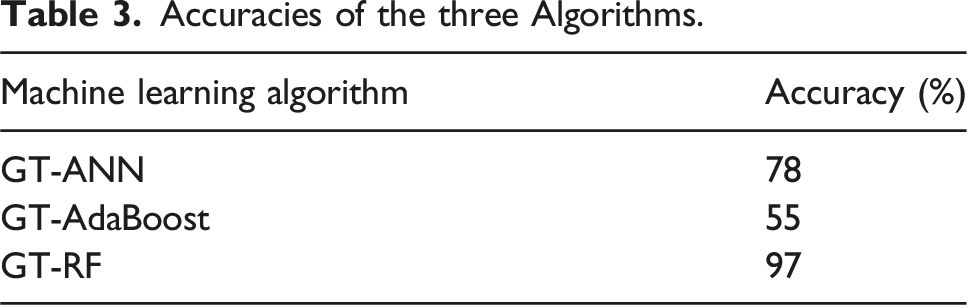
Accuracies of the three Algorithms.

Machine learning algorithm	Accuracy (%)
GT-ANN	78
GT-AdaBoost	55
GT-RF	97

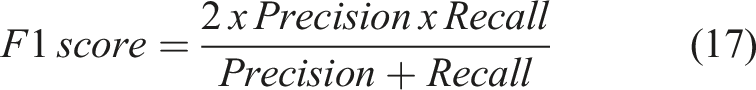
In addition to accuracy, the performance of the model can be evaluated by calculating the precision, recall, and F1 score of each class (Guo et al., 2021; Zhong et al., 2019). The values of the precision and the recall are obtained by equations (15) and (16), respectively. An F1 score is defined as the harmonic mean of precision and recall (Zhong et al., 2019). It can be calculated by equation (17).

P r e c i s i o n = \frac{N u m b e r o f c o r r e c t l y c l a s s i f i e d g r o u p s o f A E h i t s i n t h e l o a d s t e p}{T o t a l n u m b e r o f a c t u a l g r o u p s o f A E h i t s i n t h e l o a d s t e p}

(15)

R e c a l l = \frac{N u m b e r o f c o r r e c t l y c l a s s i f i e d g r o u p s A E h i t s i n t h e l o a d s t e p}{T o t a l n u m b e r o f g r o u p s o f A E h i t s p r e d i c t e d i n t h e l o a d s t e p}

(16)

F 1 s c o r e = \frac{2 x P r e c i s i o n x R e c a l l}{P r e c i s i o n + R e c a l l}

(17)

For the GT-ANN, the precisions of the four load steps are respectively 100%, 100%, 10%, and 100% from L2 to L5. While the recalls are respectively 100%, 100%, 53%, and 100% from L2 to L5. The F1 scores of the four load steps are respectively 100%, 69%, 18%, and 100% from L2 to L5. Moreover, the precisions of the four load steps, L2 to L5, for the GT-AdaBoost are 100%, 0%, 15%, and 100%, respectively. The recalls are respectively 100%, 0%, 100%, and 35% from L2 to L5. The F1 scores are respectively 100%, 0%, 26% and 58% from L2 to L5. The precision, recall, and F1 score for each load step was calculated for the GT-RF. Precisions of the four load steps are respectively 100%, 95%, 93%, and 100%. Recalls of the four load steps are respectively 97%, 100%, 98%, and 93%. F1 scores of the four load steps are 98.5%, 97.4%, 95.4%, and 96.4%, respectively. Figure 18 presents the evaluation of each load step for the three machine learning algorithms.

Figure 18.

Evaluation for each load step (a) GT-ANN; (b) GT-AdaBoost; (c) GT-RF.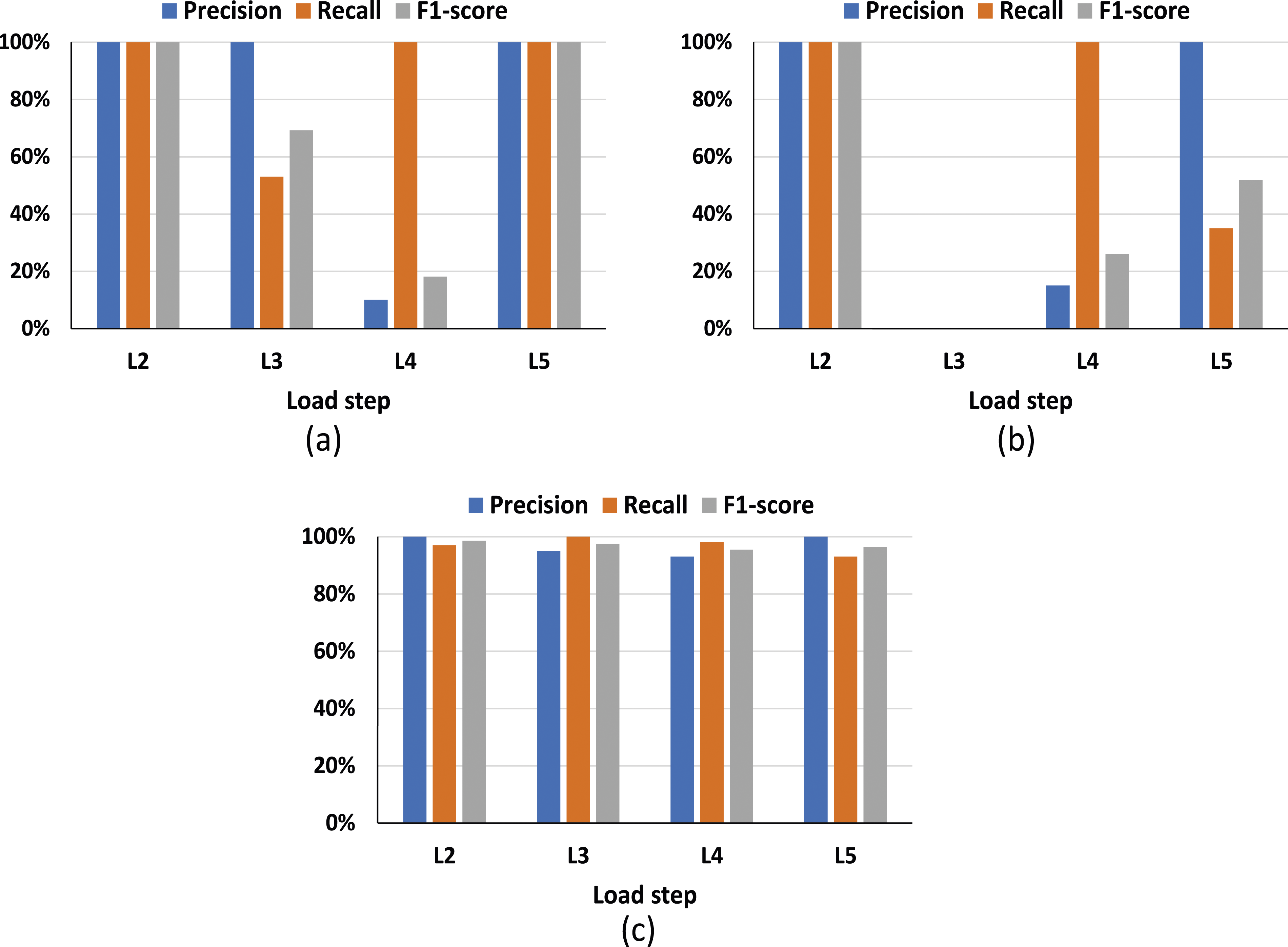

The F1 scores obtained by the three different machine algorithms are shown in Figure 19. It can be observed that the F1 scores of four load steps attained by the ANN and AdaBoost show a wide variety. However, the F1 scores obtained by the random forest are relatively stable. In addition, the F1 scores of random forest are higher than ANN and AdaBoost. Hence, the random forest has the best performance for classifying the AE hits in each load step.

Figure 19.

Comparison of F1 scores.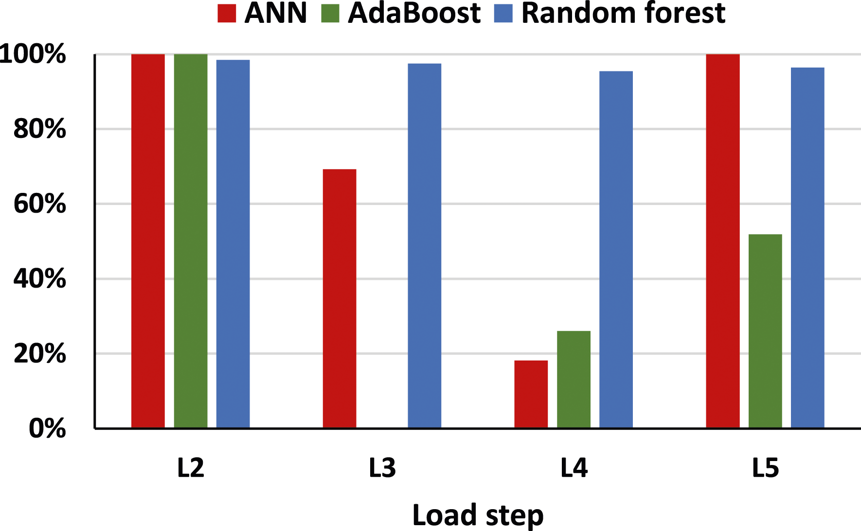

The performance of the random forest algorithm was better than the ANN and AdaBoost algorithms in classifying the AE hits to their corresponding load steps. One possible explanation could be related to how each machine-learning model deals with outliers. In machine learning, outliers are data points that differ from most of the data points in a data set. 15 AE parameters were fed to the machine learning models to classify the data points.

AdaBoost is an ensemble learning method designed to enhance the performance of multiple weak learning models, referred to as decision stumps. During the AdaBoost process, each stump is trained over multiple iterations, resulting in a weighted function. At the end of these iterations, each stump receives a weight. The final classification is determined by a vote from all the stumps, considering their respective weights. AdaBoost can be impacted by outliers. This is due to outliers receiving higher weights in the iterative process, having a more significant impact on the final model. Similarly, ANN can be affected by outliers, potentially leading to a poor performance. Outliers can mislead the model during training, causing it to overfit the training data. The model may try to fit the outliers, resulting in inaccurate weight updates. This will result in poor performance when subjected to the testing data.

On the other hand, random forest is an ensemble learning algorithm, specifically a bagging algorithm. It leverages multiple weak learning models, which are decision trees, to make predictions. The strength of this algorithm lies in the way it determines its final prediction: by averaging the outcomes of these decision trees. This approach helps mitigate the risk associated with individual trees making errors. In addition, random forests consider only a subset of features when constructing each decision tree, which effectively lessens the influence of outliers, resulting in a better classification outcome. This can be demonstrated by the performance of the three machine learning algorithms employed in this study.

Robustness of the random forest model

The performance of random forest algorithm was better than the artificial neural network (ANN) and AdaBoost algorithms in classifying the AE hits to their corresponding load steps. Three different scenarios were employed to evaluate the performance of the model when tested on data from another girder. First, the random forest algorithm was trained on the AE data collected from five different girders (T1, T2, T3, T4, and T5) and tested on the AE data collected from another girder (T6). Figure 20 presents the results of the classification of the AE hits. For the data produced by L2, the number of AE hits accurately classified to L2 was 158, whereas 38, 2, and 0 were misclassified to L3, L4, and L5, respectively. Since the maximum number of AE hits was allocated to L2 for this group of AE hits, the probability of those AE hits being allocated to L2 is the highest. Thus, this group of AE hits was accurately classified as L2. Following the same decision-making process, the AE data generated by L3 and L4 were misclassified into L2. In addition, the AE data generated by L5 was correctly classified into L5.

Figure 20.

Output of random forest trained on data from five girders and tested on another girder.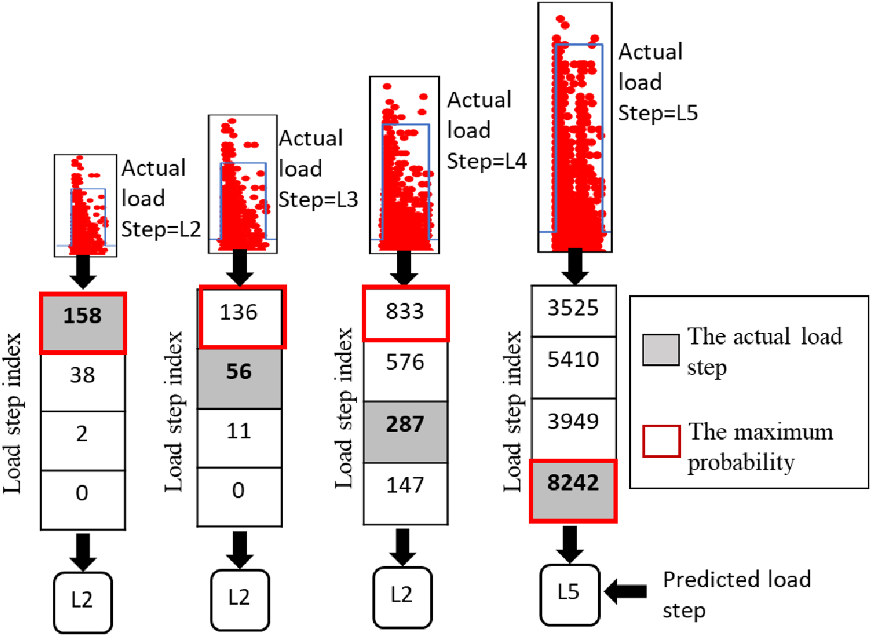

Second, the random forest algorithm was trained on the AE data collected from eight different girders (T1, T2, T3, T4, T5, T7, T8, and T9) and tested on the AE data collected from another girder (T6). Figure 21 presents the results of the classification of the AE hits. For the data produced by L2, the number of AE hits accurately classified to L2 was 170, whereas 16, 11, and one were misclassified to L3, L4, and L5, respectively. Since the maximum number of AE hits was allocated to L2 for this group of AE hits, the probability of those AE hits being allocated to L2 is the highest. Thus, this group of AE hits was accurately classified as L2. Following the same decision-making process, the AE data generated by L4 and L5 were correctly classified into L4 and L5, respectively. In addition, the AE data generated by L3 was incorrectly classified into L2. The results show that increasing the training data of the model provided a better performance for the model to classify AE hits to their corresponding load steps. Hence, a broader and more diverse data set is required to attain further enhancements in performance on different girders.

Figure 21.

Output of random forest trained on data from eight girders and tested on another girder.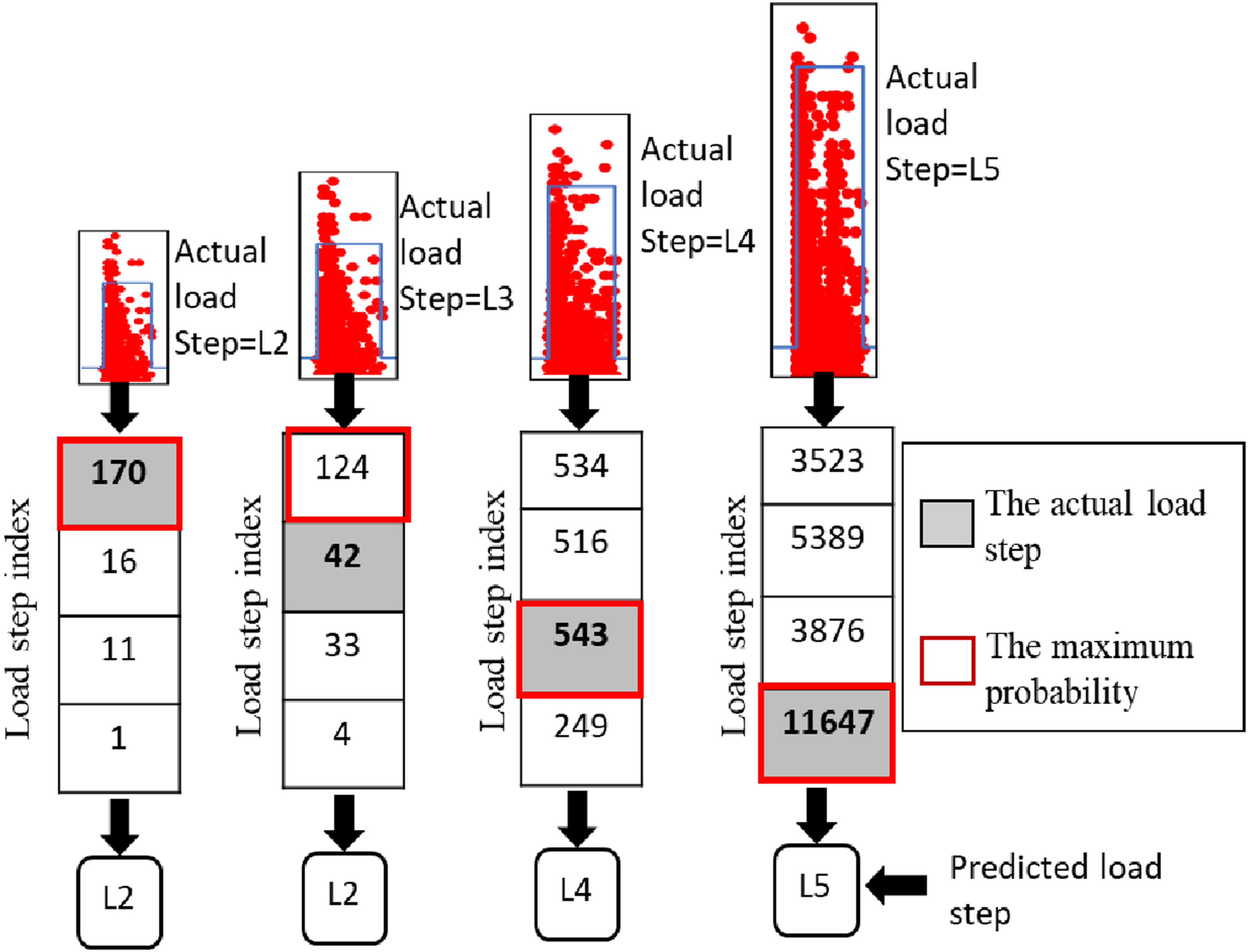

Third, the random forest algorithm was trained on the AE data collected from nine different girders (T1, T2, T3, T4, T5, T6, T7, T8, and T9) and tested on the AE data collected from a random sample from all the girders. Figure 22 presents the results of the classification of the AE hits. Following the same decision-making process, the AE data generated by L2, L3, L4, and L5 were correctly classified into L2, L3, L4, and L5, respectively. The results show that including representative training data from each girder for the model can help to increase the performance of the model. The model correctly classified the AE hits to their corresponding load steps.

Figure 22.

Output of random forest trained on data from nine girders and tested on random sample.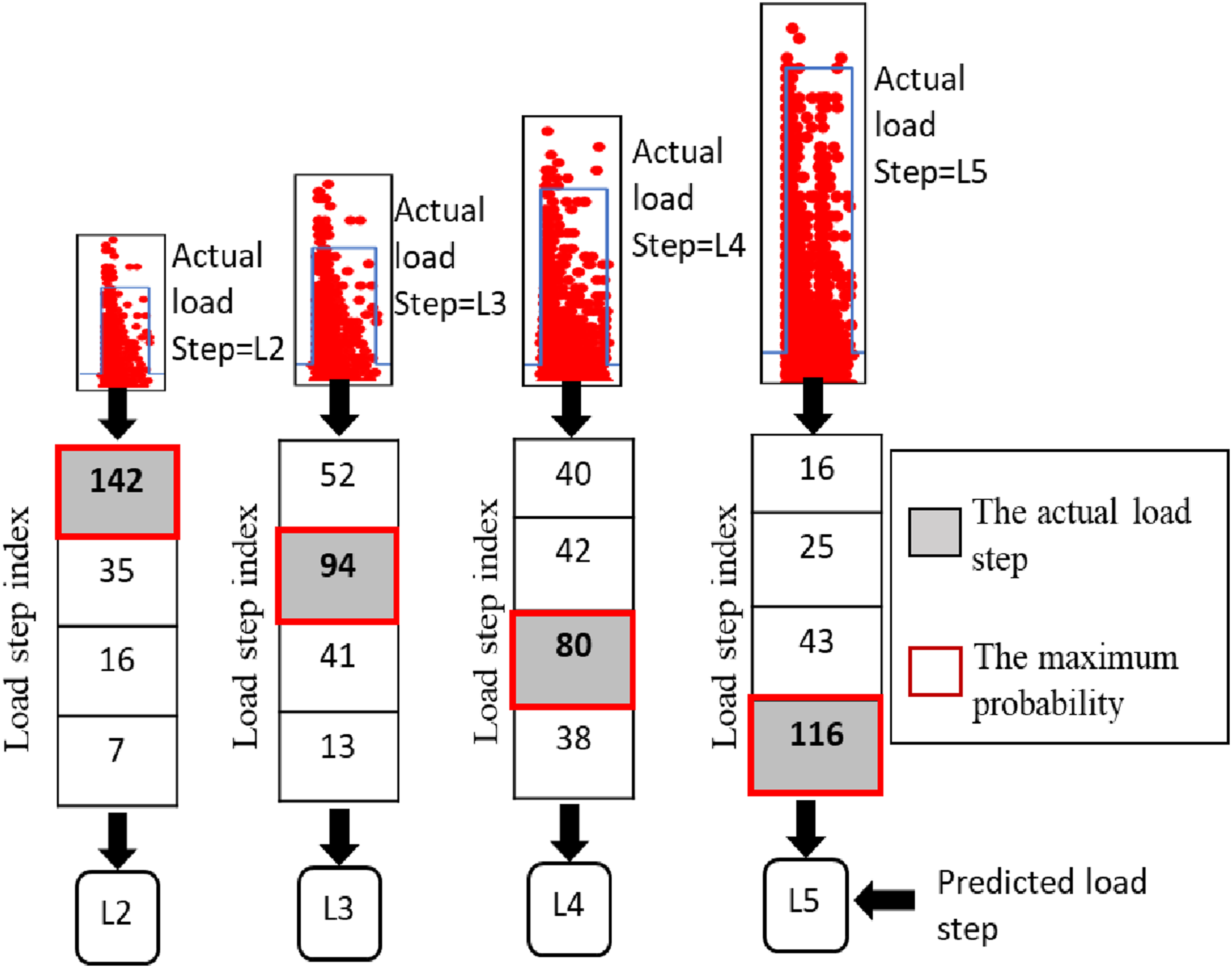

Conclusions

AE data was collected from flexural tests of prestressed concrete girders. This paper considered three improved machine learning approaches to classify AE hits to their corresponding load steps (theoretical vehicle loads). BT-ANN, BT-AdaBoost, and BT-RF were used, and their performance was compared. The main conclusions of the paper are summarized as follows:

(1) Balanced training for the training data is essential to resolve the imbalance issue when unequal data sets are fed to the machine learning model. Since the machine learning model can be biased in the classification to the largest data set.

(2) The performance of the BT-RF algorithm was better than BT-ANN and BT-AdaBoost algorithms in classifying the AE hits to their corresponding load steps. The BT-RF had an overall accuracy of 97%, whereas the BT-ANN and BT-AdaBoost models had an accuracy of 78% and 55%, respectively.

(3) AE in conjunction with improved random forest may potentially be used to determine the vehicle loads on bridge girders. Furthermore, incorporating representative training data enhances model performance. To achieve further improvements across different girders, a broader and more diverse dataset is necessary.

This study is limited to a nine 30 ft long prestressed reinforced concrete girder. Since AE sensors depend on the surface properties to which they are attached, more research must be done on other typical structures. In addition, this study is limited to the application of a static load, whereas the vehicle loads are dynamic. Hence, future studies should focus on analyzing AE data acquired from the effects of dynamic loads.

Footnotes

Declaration of conflicting interests

The author(s) declared no potential conflicts of interest with respect to the research, authorship, and/or publication of this article.

Funding

The author(s) disclosed receipt of the following financial support for the research, authorship, and/or publication of this article: This research was partially supported by the South Carolina Department of Transportation (SCDOT) under contract number SPR No. 758.

ORCID iD

Li Ai

Data Availability Statement

Data used and corresponding calculations done during the study are available from the corresponding author by request.

References

Aashto

(1998) Bridge design specifications. is a report from AASHTO. https://www.fhwa.dot.gov/publications/research/infrastructure/bridge/05056/chapt3c.cfm.

Aggelis

Verbruggen

Tsangouri

, et al. (2013) Characterization of mechanical performance of concrete beams with external reinforcement by acoustic emission and digital image correlation. Construction and Building Materials 47: 1037–1045.

Soltangharaei

Bayat

, et al. (2021) Source localization on large-scale canisters for used nuclear fuel storage using optimal number of acoustic emission sensors. Nuclear Engineering and Design 375: 111097.

Soltangharaei

Bayat

, et al. (2021) Detection of impact on aircraft composite structure using machine learning techniques. Measurement Science and Technology 32(8): 084013.

Bahari

Shahidan

Abdullah

, et al. (2017) Crack classification in concrete beams using AE parameters. In: IOP Conference Series: Materials Science and Engineering.

Breiman

(2001) Random forests. Machine Learning 45: 5–32.

Dontu

Barsanescu

Andrusca

, et al. (2020) Weigh-in-motion sensors and traffic monitoring systems-Sate of the art and development trends. In: IOP Conference Series: Materials Science and Engineering. IOP Publishing, Vol. 997, No. 1, p. 012113.

ElBatanouny

Mangual

Ziehl

, et al. (2014) Early corrosion detection in prestressed concrete girders using acoustic emission. Journal of Materials in Civil Engineering 26(3): 504–511.

ElBatanouny

Ziehl

Larosche

, et al. (2014) Acoustic emission monitoring for assessment of prestressed concrete beams. Construction and Building Materials 58: 46–53.

10.

Elbatanouny

(2023) Load determination, strengthening, and Behavior study of prestressed concrete channel bridge girders in South Carolina. https://scholarcommons.sc.edu/etd/7628/.

11.

Elbatanouny

Henderson

, et al. (2024) Condition assessment of prestressed concrete channel bridge girders using acoustic emission and data-driven methods. Structures.

12.

Erb

(1993) Introduction to backpropagation neural network computation. Pharmaceutical research 10: 165–170.

13.

Guo

Qian

, et al. (2021) Automatic railroad track components inspection using real‐time instance segmentation. Computer-Aided Civil and Infrastructure Engineering 36(3): 362–377.

14.

Hearn

(2014) State bridge load posting processes and practices. https://nap.nationalacademies.org/catalog/22412/state-bridge-load-posting-processes-and-practices.

15.

Hecht-Nielsen

(1992) Theory of the Backpropagation Neural Network Neural Networks for Perception. Elsevier, 65–93.

16.

Holford

Eaton

Hensman

, et al. (2017) A new methodology for automating acoustic emission detection of metallic fatigue fractures in highly demanding aerospace environments: an overview. Progress in Aerospace Sciences 90: 1–11.

17.

Hou

Jeong

Lynch

, et al. (2022) Data-driven analytical load rating method of bridges using integrated bridge structural response and weigh-in-motion truck data. Mechanical Systems and Signal Processing 163: 108128.

18.

Jordan

Mitchell

(2015) Machine learning: trends, perspectives, and prospects. Science 349(6245): 255–260.

19.

Laxman

Ross

, et al. (2023) Determination of vehicle loads on bridges by acoustic emission and an improved ensemble artificial neural network. Construction and Building Materials 364: 129844.

20.

Nie

J-H

Wang

, et al. (2023) Damage location, quantification and characterization of steel-concrete composite beams using acoustic emission. Engineering Structures 283: 115866.

21.

Lydon

Taylor

Robinson

, et al. (2016) Recent developments in bridge weigh in motion (B-WIM). Journal of Civil Structural Health Monitoring 6: 69–81.

22.

(2020) Structural health evaluation of the prestressed concrete using advanced acoustic emission (AE) parameters. Construction and Building Materials 250: 118860.

23.

Mihaila

Barsanescu

Moraras

(2022) Weigh-in-Motion sensors and traffic monitoring systems. State of the art and perspectives. Bulletin of the Polytechnic Institute of Iași. Machine constructions Section 68(1): 125–146.

24.

Nair

Cai

Kong

(2020) Using acoustic emission to monitor failure modes in CFRP-strengthened concrete structures. Journal of Aerospace Engineering 33(1): 04019110.

25.

Rätsch

Onoda

Müller

K-R

(2001) Soft margins for AdaBoost. Machine Learning 42: 287–320.

26.

Sandri

Zuccolotto

(2006) Variable selection using random forests. In: Data Analysis, Classification and the Forward Search: Proceedings of the Meeting of the Classification and Data Analysis Group (CLADAG) of the Italian Statistical Society. University of Parma. June 6–8, 2005.

27.

Schapire

(2013) Explaining Adaboost Empirical Inference: Festschrift in Honor of Vladimir N. Vapnik. Springer, 37–52.

28.

Soltangharaei

Anay

, et al. (2020) Temporal evaluation of ASR cracking in concrete specimens using acoustic emission. Journal of Materials in Civil Engineering 32(10): 04020285.

29.

Soltangharaei1a

Hill

, et al. (2020) Acoustic emission technique to identify stress corrosion cracking damage. Structural Engineering & Mechanics 75(6): 723–736.

30.

Tan

Bao

Zhang

, et al. (2021) Strain transfer effect in distributed fiber optic sensors under an arbitrary field. Automation in Construction 124: 103597.

31.

Tan

Guo

Zou

, et al. (2022) Buckling detection and shape reconstruction using strain distributions measured from a distributed fiber optic sensor. Measurement 200: 111625.

32.

Tsai

C-P

Lee

T-L

(1999) Back-propagation neural network in tidal-level forecasting. Journal of Waterway, Port, Coastal, and Ocean Engineering 125(4): 195–202.

33.

Uddin

Zhao

Waldron

, et al. (2011) Weigh-in-motion (WIM) Data for Site-specific LRFR Bridge Load Rating. University Transportation Center for Alabama.

34.

Vandecruys

Martens

Van Steen

, et al. (2022) Preliminary results on acoustic emission and vibration-based monitoring of locally corroded reinforced concrete beams. Proceedings of the The International Symposium on Nondestructive Testing in Civil Engineering. NDT. net, No. 2022-09.

35.

Wang

J-Z

Wang

J-J

Zhang

Z-G

, et al. (2011) Forecasting stock indices with back propagation neural network. Expert Systems with Applications 38(11): 14346–14355.

36.

Wang

Lei

Zhang

, et al. (2016) Machine learning basics. Deep learning: 98–164.

37.

Worley

Dewoolkar

Xia

, et al. (2019) Acoustic emission sensing for crack monitoring in prefabricated and prestressed reinforced concrete bridge girders. Journal of Bridge Engineering 24(4): 04019018.

38.

Zeng

Hartell

Soliman

(2020) Damage evaluation of prestressed beams under cyclic loading based on acoustic emission monitoring. Construction and Building Materials 255: 119235.

39.

Zhong

Zhou

(2019) Deep learning based multi-temporal crop classification. Remote sensing of environment 221: 430–443.

40.

Zhou

Shan

Liu

, et al. (2021) Fracture characterization of composite slabs with different connections based on acoustic emission parameters. Structural Control and Health Monitoring 28(4): e2703.

41.

Zhu

Sun

Malone

, et al. (2021) Online Monitoring System for Concrete Structures Affected by Alkali-Silica Reaction: Univ. Of Nebraska. Lincoln, NE (United States).

An automated load determination approach for concrete girder bridges through acoustic emission

Abstract

Keywords

Introduction

Experimental setup

Specimens

Test setup

Acoustic emission

Data processing and methodology

Framework

Artificial neural network

AdaBoost

Random forest

Results and discussion

Performance of BT-ANN

Performance of BT-AdaBoost

Performance of BT-RF

Comparison and discussion

Robustness of the random forest model

Conclusions

Footnotes

Declaration of conflicting interests

Funding

ORCID iD

Data Availability Statement

References