From Doppler to duplex: A personal early history of the vascular laboratory

Abstract

In the mid-1970s, a group of clinicians and bioengineers at the University of Washington, under the direction of Dr D Eugene Strandness, Jr, built a prototype duplex scanner that combined B-mode imaging and pulsed Doppler flow detection in a single instrument. At that time, I was a general surgery resident with an interest in vascular disease, and arrangements were made for me to spend a year in the Strandness laboratory. The prototype duplex system was just being completed when I arrived in 1978, and I immediately became involved in a series of validation studies in which patients with carotid disease were scanned and spectral waveform parameters were correlated with independently read contrast arteriograms. This work resulted in the University of Washington duplex criteria for carotid artery disease, which have been widely adopted and modified. Subsequent advances in ultrasound technology expanded the applications of duplex scanning to the peripheral arteries and veins, as well as the abdominal vessels. In 1984, I joined Dr Strandness on the faculty in the Department of Surgery at the University of Washington where I have remained throughout my career. Over the years, I have had the opportunity to participate in many important developments, described in this article, that have helped to make the vascular laboratory the essential clinical resource that it is today.

Introduction

I graduated from the Johns Hopkins University School of Medicine in May 1976 and started my general surgery residency in July at the University of British Columbia in Vancouver, Canada. My plan was to finish general surgery and apply to fellowships in cardiothoracic surgery. I had little exposure to vascular surgery as a medical student, but my first rotation as a resident was on a service with several busy vascular surgeons, and I found the vascular cases extremely interesting. The vascular surgery group at Vancouver General Hospital was also starting a clinical vascular laboratory, and I volunteered to help in any way I could. At that time, vascular laboratories were small and mostly associated with vascular surgery practices, and there was not much information available on how to ‘set up’ a laboratory. In an effort to obtain some additional guidance, arrangements were made for me to spend time in the laboratory of Dr D Eugene Strandness, Jr, a recognized expert in the new field of noninvasive vascular testing, at the University of Washington in Seattle.

I arrived at the University of Washington in September 1978 and, after some introductions, Dr Strandness escorted me to a large room with several racks of electronic components and a table with a thin mattress and a small pillow. He described all this as the new duplex ultrasound scanner that was being built by the bioengineers and told me that I would be using this instrument to evaluate patients with carotid artery disease. The rest, as the saying goes, ‘is history’.

The concept of nondestructive testing

Dr Strandness graduated from the University of Washington School of Medicine in 1954 and then began his general surgery residency at the same institution. Although he had intended to specialize in gastrointestinal surgery, he was assigned to spend his mandatory residency research year studying vascular disease. In 1990, reflecting on that very early experience, Dr Strandness recalled, ‘In trying to generate ideas and projects, I was horrified to find that the only tools available to me were my fingers, eyes, ears, and arteriography … I decided to turn to our physiologists, who spend their lives measuring things, to see if they could help’. ¹

Fortuitously, as Dr Strandness was starting his vascular studies, Dr Robert Rushmer, a Professor of Physiology and Biophysics at the University of Washington, was working on quantitative methods for studying cardiovascular function in ‘intact’ animals. One approach was an ultrasonic flowmeter based on the Doppler principle that could be used with ‘no pain, hazard, or damage to the skin’. ² This introduced the concept of ‘nondestructive’ testing, a term that originally described methods used for industrial purposes, which was later replaced by ‘noninvasive’ testing in medical settings. Dr Rushmer offered a 3-month course on the application of engineering and electronic methods in medical research, and it was through this course that Dr Strandness first learned about ultrasonography and other noninvasive techniques for measuring blood flow. It soon became clear that these physiologic or functional tests could bridge the gap between the subjective vascular physical examination and the anatomic information provided by invasive arteriography. This led to a longstanding and productive collaboration between the vascular surgery and bioengineering groups at the University of Washington.

Early Doppler technology

In 1961, Dr Rushmer’s group described the use of ultrasonic flowmeters in animals, and the first clinical applications of a transcutaneous Doppler flowmeter in humans were reported in the mid-1960s (Figure 1).^2,3–6 After completing his general surgery residency, a period of service in the US Air Force, and a research fellowship at the National Heart Institute, Dr Strandness joined the faculty in the Department of Surgery at the University of Washington in 1964. A detailed description of the evaluation of patients with vascular disease using the ultrasonic Doppler velocity detector was published by the University of Washington group in 1967. ⁶ Interpretation of the Doppler signals was done primarily by ‘audible’ analysis (i.e. listening to the amplified Doppler-shifted frequencies) with the examiner learning to differentiate between the sounds of normal and abnormal flow patterns. This report included 84 arterial cases and 17 venous cases, and some of the specific applications described were localization of arterial and venous occlusions, estimation of arterial occlusion length, assessing the results of operative interventions, and evaluation of edema in the extremities. ⁶

Figure 1.

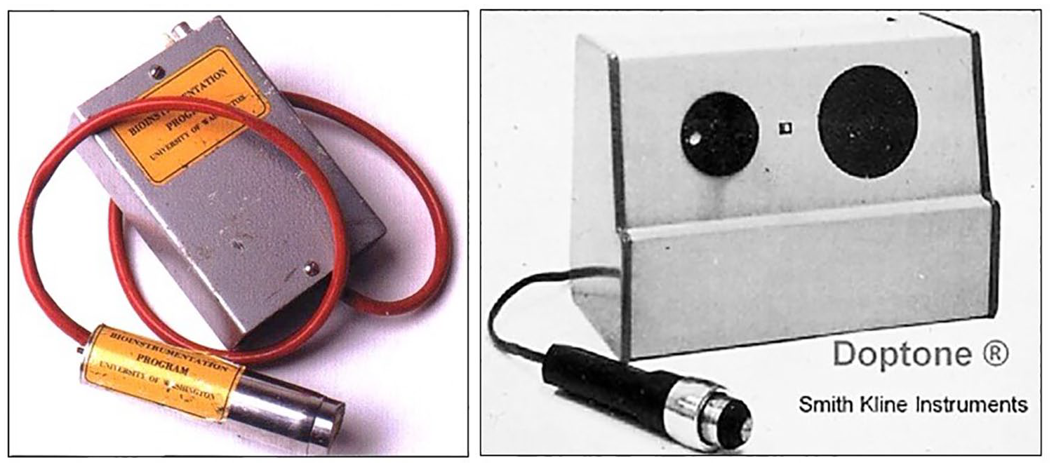
(Left) Prototype continuous wave Doppler system developed at the University of Washington in the 1960s. (Right) First commercially produced Doppler system based on this prototype made by the Smith Kline Instrument company and marketed as the ‘Doptone’, which sold for around $300 in 1965. From ref. 6, with permission from Elsevier. © 1967 Elsevier Inc.

The early continuous wave Doppler system showed promise as a noninvasive diagnostic tool, but it had three significant limitations. ⁷ First, it could not determine flow direction with respect to the ultrasound probe. Animal studies had shown that the pulse cycle in peripheral arteries consisted of forward and reverse flow components, and detection of reflux in veins would require the ability to distinguish between forward and reverse flow. The second limitation was the lack of a graphical method for recording and displaying the flow information. Although audible analysis was useful in the clinical setting, it was purely qualitative and made documentation difficult. Finally, the continuous wave Doppler detected flow along the entire path of the ultrasound beam, so there was no way to sample flow selectively at specific depths in tissue.

All these limitations would be overcome by incremental advances in ultrasound technology. Directional continuous wave Doppler systems were developed by separating the positive and negative Doppler shifts associated with forward and reverse flow components. The initial method for generating analog waveforms from the continuous wave Doppler-shifted signal used a zero-crossing detector. A better method for displaying the Doppler waveforms was spectral analysis, which separated the Doppler-shifted signal into component frequencies and showed the entire frequency and amplitude content over time. However, in the 1960s, spectral analysis was a complicated and slow process that required recording the Doppler signals on magnetic tape, sending them to Northrop Nortronics in Needham Heights, MA, and waiting several weeks to receive the processed tapes with the spectral waveforms. ⁶ The subsequent development of the Fast Fourier Transform (FFT) spectrum analyzer would provide a practical method for obtaining spectral waveforms in real-time. Lack of depth resolution was an inherent feature of continuous wave Doppler instruments. The ability to selectively sample flow along the ultrasound beam required the development of a pulsed Doppler system which was based on radar principles and the relatively constant speed of ultrasound in tissue. ⁸

Pulsed Doppler and ultrasonic arteriography

In 1971, D Eugene Hokanson, a physicist working with Dr Strandness at the Seattle VA Medical Center, designed and built a pulsed Doppler imaging system that could produce a ‘flow image’ of vascular structures.^9,10 This device used a 5 MHz directional pulsed Doppler with multiple sample volumes or range gates which could be moved along the Doppler beam to locate areas of flow. The pulsed Doppler transducer was mounted on a position-sensing mechanical arm, and by moving the transducer over the skin, and adjusting the depth of the sample volumes, a two-dimensional flow image of the vessels could be created on an oscilloscope screen (Figure 2). This approach was used to evaluate flow in the extracranial carotid arteries, as well as the common femoral, deep femoral, superficial femoral, and popliteal arteries. ¹¹ Although it was initially hoped that the pulsed Doppler imaging system might yield diagnostic information comparable to contrast arteriography, the anatomic accuracy of the flow images was relatively poor. In 1973, Mr Hokanson founded D. E. Hokanson, Inc. to develop and market his own instruments for vascular research and diagnosis, including the new ‘Ultrasonic Arteriograph’. This instrument was never a major commercial success, but it was an important technical step toward more sophisticated direct noninvasive vascular testing.

Figure 2.

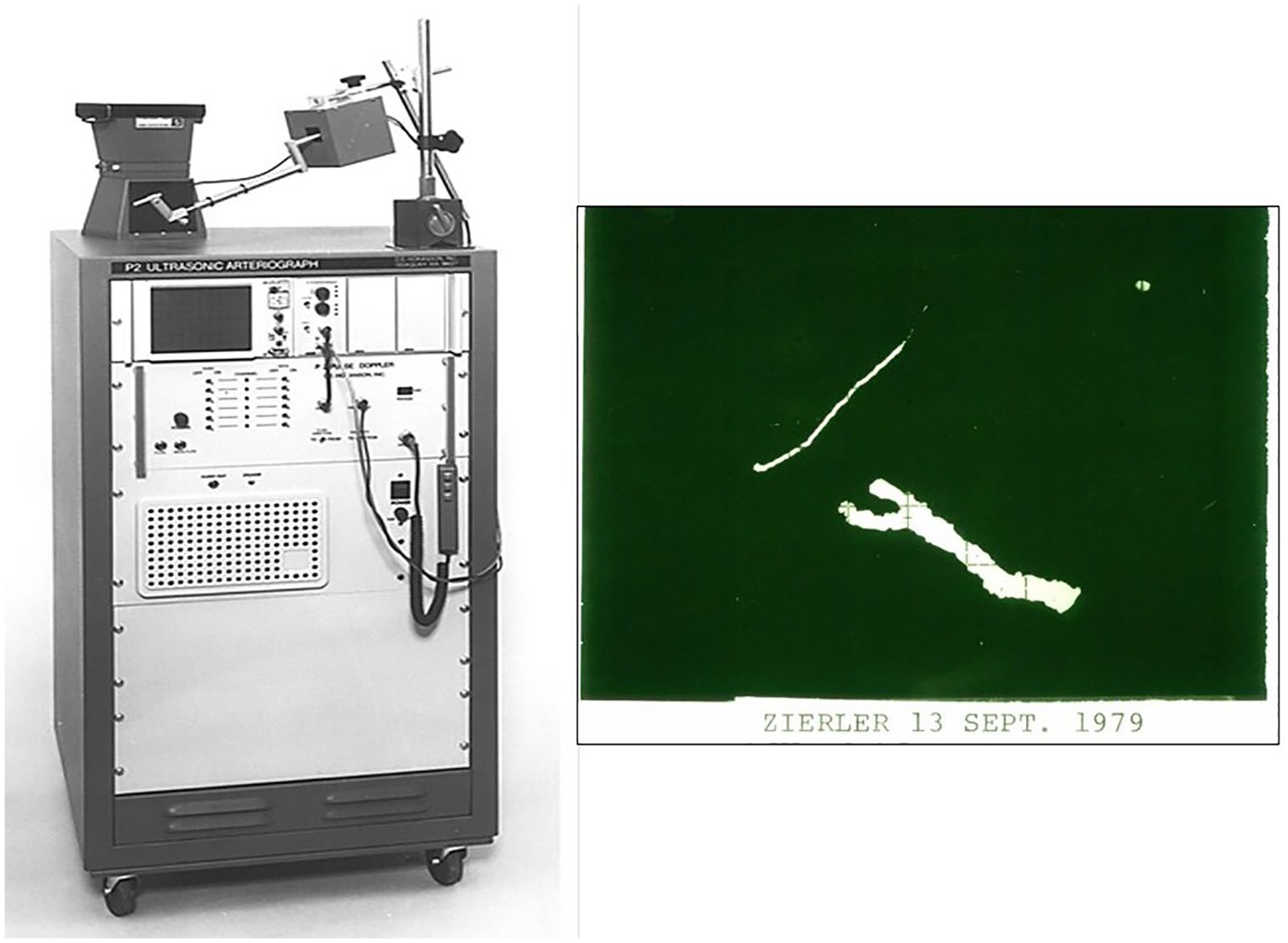
(Left) The Ultrasonic Arteriograph built and marketed by D. E. Hokanson, Inc. in the early 1970s. The position-sensing mechanical arm with the Doppler transducer and Polaroid camera for recording images are on top of the cabinet. Image reproduced courtesy of Kyra Gray, D. E. Hokanson, Inc. (Right) Flow image of the author’s right carotid bifurcation taken with the Ultrasonic Arteriograph on September 13, 1979. The diagonal line represents the lower border of the mandible. From Zierler RE. Carotid duplex criteria: What have we learned in 40 years? Semin Vasc Surg 2020; 33: 36–46, with permission from Elsevier. © 2020 Elsevier Inc.

Ultrasound and atherosclerosis

As more sophisticated Doppler techniques were being developed, Dr Strandness and his collaborators were investigating other ultrasound methods for visualizing blood vessels. It was recognized that atherosclerotic plaques contain calcium, and even microscopic calcium deposits produced significant attenuation of ultrasound. Based on some initial experiments using arterial segments removed at autopsy and a very crude scanning system, B-mode imaging showed some promise for characterizing arterial lesions. ¹²

In the mid-1970s, a prototype B-mode scanning system was built at the University of Washington that contained three 5 MHz fixed-focus ultrasound transducers mounted on a rotating wheel, with the focal point of each transducer located about 2 cm below the skin surface. The transducers pointed out radially, and each transducer would ‘sweep out’ a two-dimensional sector image of the underlying tissue as the wheel rotated. These serial images were combined electronically to create a real-time B-mode image. An image of a carotid bifurcation from one of the first patients evaluated with this device is shown in Figure 3. Although the image quality is poor by modern standards, the carotid bifurcation can be seen in a longitudinal view with the common carotid, internal carotid, and external carotid branches all visualized and apparently patent. Unexpectedly, when this patient had an arteriogram, the internal carotid artery was found to be occluded. This experience indicated that at least some thrombus and plaque had acoustic properties similar to those of flowing blood and therefore could not be reliably identified by B-mode imaging alone. Since the difficulty appeared to be in determining whether an artery was patent or occluded, it seemed logical to use a Doppler system to detect flow in the imaged vessels. It was this single case that led to the concept of combining real-time B-mode imaging and pulsed Doppler flow detection in a single instrument. ¹³ As Dr Strandness observed in 1996, ‘The term ‘duplex’ (B-mode and Doppler) was adopted and has remained to this day as the best means of describing the system itself and what it is capable of doing’. ⁷

Figure 3.

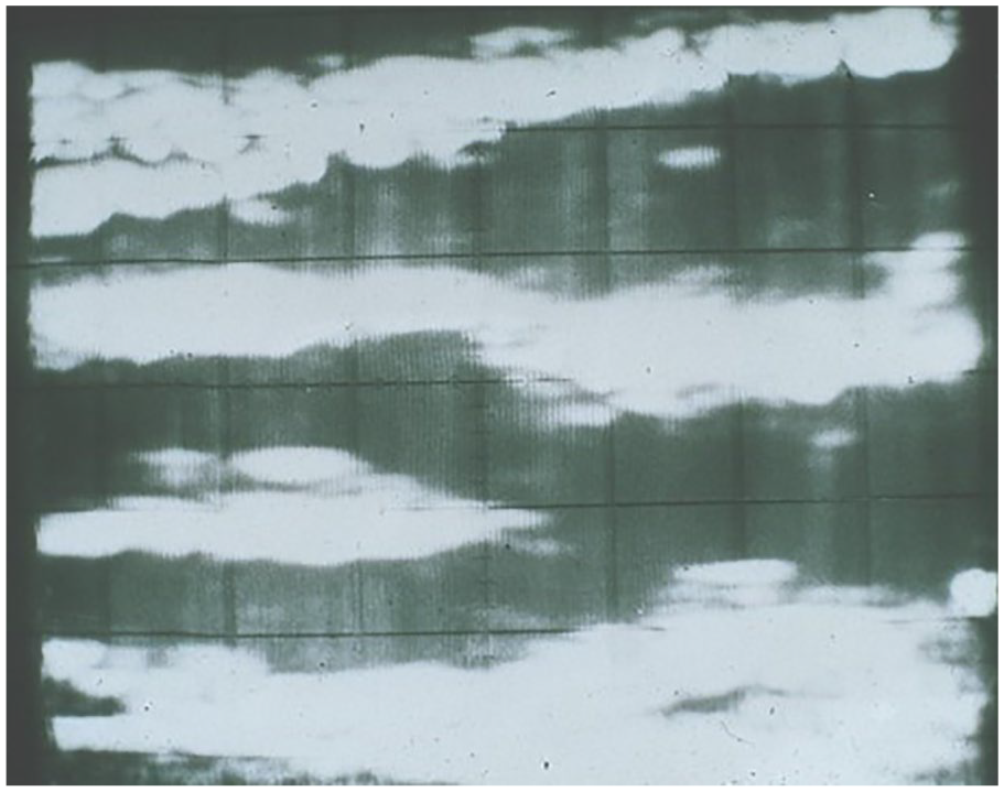
Real-time B-mode ultrasound image of a carotid bifurcation obtained with the prototype scanning system. The carotid bifurcation is displayed in longitudinal view with the common carotid on the right, the internal carotid on the bottom left, and the external carotid on the top left. From Zierler RE. Carotid duplex criteria: What have we learned in 40 years? Semin Vasc Surg 2020; 33: 36–46, adapted with permission from Elsevier. © 2020 Elsevier Inc.

The prototype duplex ultrasound scanner

The University of Washington prototype B-mode scanning system was modified to create the first duplex ultrasound scanner (Figure 4). One of the major engineering challenges in designing this instrument was to integrate the pulsed Doppler and B-mode functions in the scanhead. ¹³ A single range gate pulsed Doppler transducer was mounted on one side of the scanhead, and a water-filled rubber ‘boot’ was used for acoustic coupling between the B-mode and Doppler transducers and the skin surface. The Doppler transducer was aligned to detect flow in the plane of the B-mode image, and the position of the Doppler beam and the pulsed Doppler sample volume were indicated by a line and a dot, respectively, superimposed on the B-mode image (Figure 5).

Figure 4.

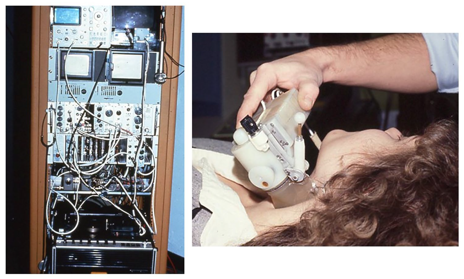
(Left) Instrument rack for the University of Washington prototype duplex scanner. The black and white television set used for viewing images is located in the upper right corner behind the scanhead. Images were stored on a Sony Betamax video recorder at the bottom of the rack. (Right) Close-up of the prototype scanhead containing three B-mode transducers on a rotating wheel and a single range gate pulsed Doppler mounted separately on the diagonal arm; a water-filled rubber ‘boot’ was used for acoustic coupling.

Figure 5.

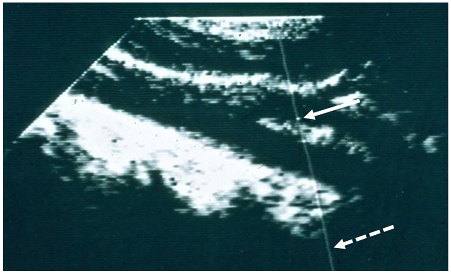
Image from the prototype duplex scanner. The position of the Doppler beam is indicated by a line (dashed arrow) and the location of the sample volume is indicated by a dot on that line (solid arrow). By moving the diagonal arm on the scanhead (Figure 4) and adjusting the depth of the sample volume, flow could be sampled at any site in the B-mode image. From Zierler RE. Carotid duplex criteria: What have we learned in 40 years? Semin Vasc Surg 2020; 33: 36–46, adapted with permission from Elsevier. © 2020 Elsevier Inc.

The prototype duplex scanner made it possible to directly visualize the extracranial carotid arteries and sample flow at selected sites within the vessels. A Honeywell FFT spectrum analyzer was used to process the pulsed Doppler signals and provide spectral waveforms. In the late 1970s, there was considerable interest in carotid artery atherosclerosis as a cause of stroke, and carotid endarterectomy was being done for patients who were found to have severe carotid stenosis with the expectation that strokes would be prevented. This was the state of the noninvasive vascular laboratory when I arrived at the University of Washington in 1978 and Dr Strandness showed me the prototype duplex ultrasound scanner.

Spectral waveforms, velocities, and flow patterns

I was one of several research fellows assigned to work on the duplex scanner project. Our job was to scan patients, collect the Doppler data, and figure out how to use the Doppler information to classify the severity of carotid disease. In those days, patients with carotid artery disease were likely to undergo catheter contrast arteriography, providing a ‘gold standard’ for assessing disease severity and correlation with the Doppler velocity parameters. The prototype scanhead was heavy and bulky, and the electric motor caused a very noticeable vibration, so it was referred to as the ‘trash masher’. The images were viewed on a small black and white television set that had been brought in by one of the bioengineers and modified for this purpose (Figure 4).

The spectral waveforms provided by the Honeywell spectrum analyzer displayed Doppler-shifted frequency in kilohertz (kHz) on the vertical axis and time on the horizontal axis, with the amplitude of the Doppler signal indicated by a gray-scale (Figure 6). The actual flow velocity (V) had to be calculated using the Doppler equation:

$$V=\frac{\mathrm{\Delta }fC}{2fcos\theta }$$

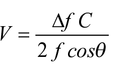
where ∆f is the Doppler-shifted frequency obtained from the spectral waveform, C is the constant speed of sound in tissue (1540 m/s), f is the frequency of the transmitted ultrasound (5 MHz), and θ is the Doppler angle. The true Doppler angle is the angle between the ultrasound beam and the direction of blood flow (or more specifically, the direction of the ultrasound reflectors which are mostly red blood cells); however, in a carotid duplex scan, the exact direction of blood flow is not known. In order to provide a clear and consistent reference for determining Doppler angle, the angle between the line of the ultrasound beam and the vessel wall, as seen in a long axis B-mode image, was used (this angle was measured by placing a plastic protractor directly on the television screen). Although it was recognized that flow is not always parallel to the vessel wall, it was believed that this approach would minimize the variability associated with Doppler velocity measurements. ¹⁴ We found that an angle of 60° was usually easy to achieve for the arteries examined in a carotid duplex scan. In addition, the cosine of 60° was 0.5, making it easy to remember. Since the velocity calculations were being done on my programmable calculator, knowing the value of the cosine was very important, so we started using a 60° Doppler angle for all carotid duplex examinations. Theoretically, it might have been better to use a somewhat smaller Doppler angle, but the 60° angle was convenient, and that is why we are now stuck with it.

Figure 6.

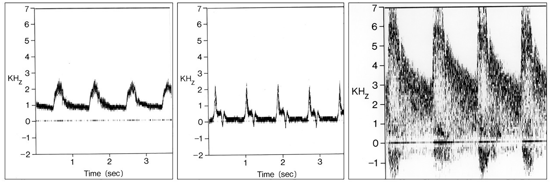
Spectral waveforms produced by the Honeywell spectrum analyzer used with the prototype duplex scanner. Doppler-shifted frequency (kHz) is on the vertical axis and time on the horizontal axis. (Left) Normal internal carotid artery waveform with forward flow throughout the cardiac cycle and a relatively narrow band of frequencies and a clear ‘window’ under the systolic peak. (Center) Waveform from a normal external carotid artery shows a ‘high resistive’ multiphasic flow pattern with a small reverse flow phase. (Right) Waveform from an internal carotid stenosis with increased peak systolic frequencies and extensive spectral broadening.

From our early experience with the prototype duplex scanning system, we learned that there were characteristic changes in velocities and flow patterns associated with arterial wall abnormalities and stenotic lesions. Wall irregularities and stenoses of less than 50% diameter reduction produced a nonlaminar or disordered flow pattern with a widening of the frequency band that was referred to as ‘spectral broadening’. Stenoses of 50% diameter reduction or more caused increases in peak systolic frequency or velocity at the site of the lesion with spectral broadening distally (Figure 6, Right). An important observation was that the high velocity jet associated with a significant stenosis was focal and tended to dissipate over only one or two vessel diameters downstream. This meant that identification of a stenosis required sampling of flow in close proximity to the lesion and led to the technique of ‘stepping through’ a stenosis by serially sampling flow patterns at closely spaced intervals along the course of the vessel.

The first carotid duplex criteria

Between 1978 and 1984, Dr Strandness and colleagues performed a series of ‘validation studies’ in which spectral waveform features were correlated with the findings on biplane carotid arteriography. For these studies, the carotid arteriograms were independently read and the maximum percent diameter reduction of the internal carotid artery was measured using calipers with the estimated normal diameter of the carotid bulb used as a reference. ¹⁵ The first threshold criterion to be established was for distinguishing between less than 50% and 50–99% internal carotid artery diameter reduction. Since it was expected that peak systolic frequency or calculated peak systolic velocity (PSV) would increase in a hemodynamically significant stenosis, the highest internal carotid PSV was determined in 135 patients (270 carotid bifurcations) having both duplex scanning and arteriography. ¹⁶ A peak systolic Doppler-shifted frequency of 4.0 kHz or greater was found to be predictive of a 50–99% internal carotid artery diameter reduction. This corresponds to a PSV threshold of 125 cm/s. Of the 103 internal carotid arteries with 50–99% diameter reduction by arteriography, 84 (81.5%) were correctly classified by the 4.0 kHz or 125 cm/s threshold, and none were classified as normal.

A spectral waveform feature that helped differentiate normal and minimally diseased internal carotid arteries was the presence or absence of ‘flow separation’ in the proximal internal carotid artery or carotid bulb.^17,18 The slight focal dilation normally present between the distal common carotid and proximal internal carotid arteries resulted in a characteristic flow pattern along the outer wall of the internal carotid (across from the apical flow divider) with low velocities and reversed or oscillating flow during each cardiac cycle. The absence of flow separation in an otherwise normal proximal internal carotid artery allowed separation of truly normal arteries from those with minimal plaque or wall thickening, features which defined the category of 1–15% diameter reduction. Internal carotid arteries with flow patterns showing no flow separation and extensive spectral broadening with peak frequencies below 4.0 kHz (or PSV < 125 cm/s) were classified as 16–49% diameter reduction.

In 1983, the University of Washington criteria for classification of internal carotid artery stenosis by duplex scanning included the following categories: normal, 1–15% diameter reduction, 16–49% diameter reduction, 50–99% diameter reduction, and occlusion. Although these categories were useful in the clinical setting, there was interest in finding a way to subdivide the 50–99% category. With the 5 MHz pulsed Doppler in the duplex scanner, the peak systolic Doppler-shifted frequencies associated with a carotid stenosis often exceeded the Nyquist limit and could not be measured accurately, but it was noted that the end-diastolic frequencies were increased with more severe degrees of stenosis. In a study of 98 internal carotid arteries with 50–99% stenosis as determined by arteriography, an end-diastolic frequency threshold of 4.5 kHz allowed separation of 50–79% stenosis and 80–99% stenosis with a positive predictive value of 70% and a negative predictive value of 94%. This end-diastolic frequency corresponds to an end-diastolic velocity of 140 cm/s. ¹⁹

As duplex scanning became more widely available in the 1980s, the University of Washington criteria for classification of internal carotid artery disease were adopted and modified by numerous vascular laboratories, and other criteria were developed independently. ²⁰ In a recent review of variation in diagnostic thresholds for carotid stenosis in 338 vascular testing centers, 60 distinct PSV thresholds were identified for degrees of stenosis ranging from ⩾ 50% to ⩾ 90%, including 15 PSV thresholds for ⩾ 50% stenosis. ²¹ So after more than four decades of carotid duplex scanning, efforts to truly standardize the criteria are ongoing. ²²

The beginnings of the modern vascular laboratory

Evaluation of the extracranial carotid arteries was the first application of the prototype and early commercial versions of the duplex scanner (Figure 7). In the mid to late 1980s, both B-mode imaging alone and duplex scanning were shown to be accurate for the diagnosis of deep vein thrombosis in the lower extremities and replaced the indirect tests for venous obstruction.^23,24 Techniques were also developed for assessing peripheral arteries with duplex scanning; however, in this testing area the indirect or physiologic tests have continued to play a significant clinical role.^25,26 Finally, the availability of low frequency convex linear array transducers made it possible to evaluate vessels in the abdomen with duplex scanning, including the renal^27,28 and mesenteric^29,30 arteries. This created a new ‘visceral vascular’ testing area for the vascular laboratory.

Figure 7.

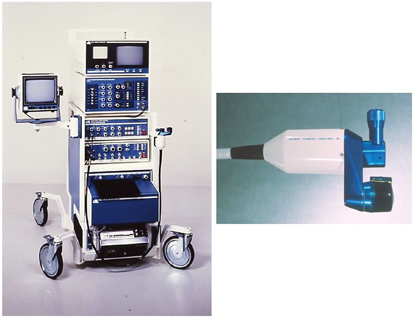
(Left) First commercial version of the duplex scanner made by Advanced Technology Laboratories (ATL) through a technology transfer agreement with the University of Washington and marketed as the ATL Mark V. ATL was acquired by Philips Electronics in 1998. (Right) Close-up of the Mark V scanhead.

These technological and clinical developments gave rise to the profession of vascular sonography. Most of the early ‘vascular technologists’ were nurses in vascular surgery practices who were asked to learn how to use the equipment and perform tests as part of their clinical duties. The American Registry for Diagnostic Medical Sonography (ARDMS) was incorporated in 1975 to provide certification examinations in medical sonography. Between 1975 and 1982, the ARDMS offered a certification examination in Peripheral Vascular Doppler, and the examination for the Registered Vascular Technologist (RVT) credential was first administered in 1983. ³¹ In 1989, I was asked to serve on the ARDMS committee responsible for the RVT examination, and over the next few years I noticed that a large number of physicians were obtaining the RVT credential. I found this perplexing, since the RVT examination evaluated the knowledge and skills required to perform vascular tests, not the interpretive or diagnostic skills used by physicians. The fact that physicians were voluntarily obtaining the RVT credential suggested that they perceived some value in formally documenting their vascular laboratory expertise.

After observing this trend, it occurred to me that there could be a role for a credential designed to evaluate what physicians actually do in the vascular laboratory. In February 2002, I wrote a letter to the ARDMS requesting that they ‘consider the feasibility of creating a new physician credential in vascular laboratory interpretation’. After a survey showed substantial interest in this concept, I was asked to chair an ARDMS committee to create the examination for this new physician credential. The credential was called the Registered Physician in Vascular Interpretation (RPVI), and the corresponding examination was the Physicians’ Vascular Interpretation (PVI). The first PVI examination was piloted in 2005, and 44 physicians earned the RPVI credential. As of January 2021, the RPVI credential has been obtained by more than 4900 physicians.

Lessons learned

In 1979, after my initial research year in Seattle, I returned to the University of British Columbia to finish my general surgery residency, but I kept in touch with the laboratory group in Seattle and continued to work on various projects. When I finished my general surgery residency in 1981, I went back to Seattle to continue my work in the Strandness laboratory and pursue further training in vascular surgery at the University of Washington. In those days there were no accredited fellowships in vascular surgery, and recognition of vascular surgery as a distinct surgical specialty was still a few years away, so a ‘fellowship’ was whatever you could arrange at an institution where there was expertise and a willingness to teach.

I finished my vascular surgery training in 1983 and accepted a position at the Wadsworth (West Los Angeles) VA Medical Center at UCLA where I had the opportunity to establish my own vascular laboratory and was the only formally trained vascular surgeon. However, shortly after I left Seattle, Dr Strandness offered me the position of Chief of the Vascular Surgery Section at the Seattle VA Medical Center, which I gladly accepted. So, in 1984, I moved to Seattle for the third time, and I have been on the University of Washington faculty continuously ever since. In 1992, I moved my primary site of practice from the Seattle VA Medical Center to the University of Washington Medical Center.

Dr Strandness died in 2002 at the age of 73. He was head of the Vascular Surgery Division at the University of Washington until 1995 and, although he retired with emeritus status at that time, he continued to run a research laboratory and see patients until a few weeks before his death. I succeeded Dr Strandness as Medical Director of the vascular laboratory at the University of Washington Medical Center, which was officially named in his honor in 2007. In retrospect, I have been fortunate to be in the right place at the right time to participate in many important developments in the vascular laboratory, and I have tried to take full advantage of those opportunities. Dr Strandness had a special proclivity for asking important clinical questions and assembling a team of trainees and colleagues to answer them. He was a steady guiding force but gave us space to express our own views and creativity. With that approach, the contributions of the University of Washington group have helped to make the noninvasive vascular laboratory the essential clinical resource that it is today. I believe that the reasons for this success are embodied in the four ‘lessons’ that Dr Strandness presented in his Presidential Address to the Society for Vascular Surgery in 1989: ¹

• Lesson 1. Do not give up too soon, cast your net widely, look outside your own field.

• Lesson 2. Do not be afraid to get some extra training, it always helps.

• Lesson 3. Take advantage of unique situations when they are presented to you. Serendipity is marvelous – take advantage of it.

• Lesson 4. There are people in this world who are not threatened by new ideas and are supportive of the work of young investigators.