Sage Journals: Discover world-class research

Abstract

Magnetic resonance imaging (MRI) has advanced significantly in the past decade and provides a safe and non-invasive method of evaluating peripheral artery disease (PAD), with and without using exogenous contrast agents. MRI offers a promising alternative for imaging patients but the complexity of MRI can make it less accessible for physicians to understand or use. This article provides a brief introduction to the technical principles of MRI for physicians who manage PAD patients. We discuss the basic principles of how MRI works and tailor the discussion to how MRI can evaluate anatomic characteristics of peripheral arterial lesions.

Keywords

angiography magnetic resonance angiography (MRA)magnetic resonance imaging (MRI)medical education vascular imaging peripheral artery disease (PAD)

Introduction

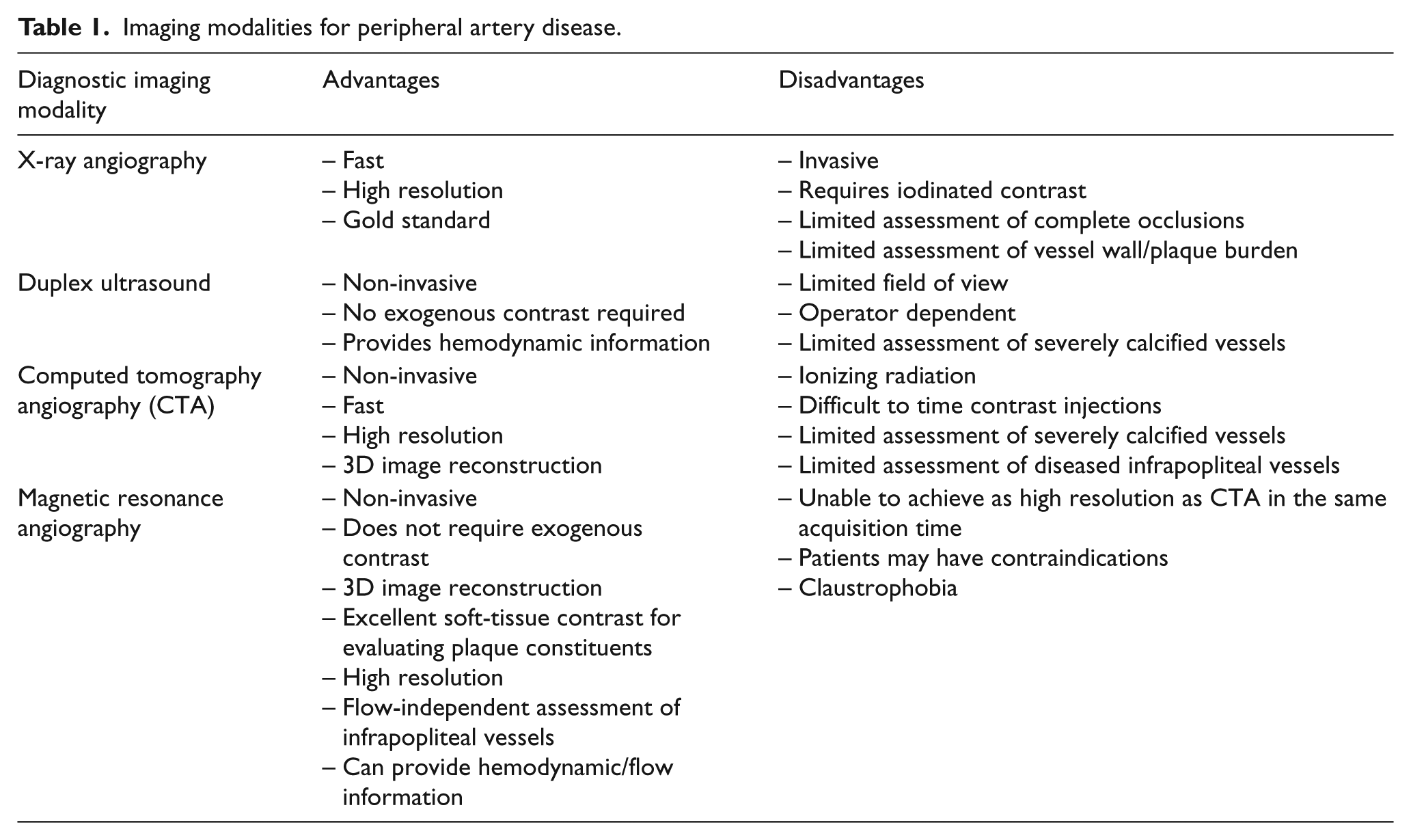
Vascular specialists rely on imaging to make treatment decisions for peripheral artery disease (PAD) patients. Anatomic characteristics of target lesions affect the durability and outcome of endovascular and surgical revascularization procedures.^1,2 According to the 2016 American Heart Association (AHA)/American College of Cardiology (ACC)³ lower extremity PAD guidelines, duplex ultrasound (DUS), computed tomography angiography (CTA), digital subtraction angiography (DSA) and magnetic resonance angiography (MRA) are all reasonable diagnostic imaging modalities to assess PAD anatomic characteristics. Each modality has advantages and limitations (Table 1) and X-ray angiography/DSA remains the gold standard for peripheral arterial imaging. Emerging magnetic resonance imaging (MRI) methods encompass many of the advantages of DUS, CTA and X-ray angiography, while addressing their limitations. MRI techniques for assessing PAD have advanced significantly in the past decade. State-of-the-art MRI techniques enable flow-independent imaging without the use of exogenous contrast agents to assess occlusive tibial vessels. New techniques can also assess peripheral arterial plaque morphology and even visualize calcium burden and morphology.

Table 1.

Imaging modalities for peripheral artery disease.

Diagnostic imaging modality	Advantages	Disadvantages
X-ray angiography	− Fast – High resolution – Gold standard	− Invasive – Requires iodinated contrast – Limited assessment of complete occlusions – Limited assessment of vessel wall/plaque burden
Duplex ultrasound	− Non-invasive – No exogenous contrast required – Provides hemodynamic information	− Limited field of view – Operator dependent – Limited assessment of severely calcified vessels
Computed tomography angiography (CTA)	− Non-invasive – Fast – High resolution – 3D image reconstruction	− Ionizing radiation – Difficult to time contrast injections – Limited assessment of severely calcified vessels – Limited assessment of diseased infrapopliteal vessels
Magnetic resonance angiography	− Non-invasive – Does not require exogenous contrast – 3D image reconstruction – Excellent soft-tissue contrast for evaluating plaque constituents – High resolution – Flow-independent assessment of infrapopliteal vessels – Can provide hemodynamic/flow information	− Unable to achieve as high resolution as CTA in the same acquisition time – Patients may have contraindications – Claustrophobia

The Society for Vascular Surgery (SVS) recently updated their anatomic lesion reporting standards¹ to include: (1) lesion length, (2) degree of stenosis/plaque burden, (3) run-off, and (4) degree of calcification. These anatomic features are important to characterize to make informed treatment decisions. In this article, we will provide an introduction to MRI physics specifically for vascular physicians by discussing how MRI can be used to evaluate these peripheral arterial lesion characteristics. We will also discuss the mechanisms behind contrast and common artifacts in images, as well as other limitations that may affect image interpretation.

MRI basic principles

Signal generation for image construction in MRI

To adequately visualize blood flowing in patent arteries, there must be signal contrast between blood in the arteries and surrounding muscle in the leg. When a patient’s leg is placed into an MRI magnet, the ‘spin’ (a quantum mechanical concept) of the protons within the leg tend to align with the magnetic field. The magnetization associated with the protons ‘precesses’ with the same motion of a wobbling spinning top. The rate or frequency (Larmor frequency) of the wobbling/precession is proportional to the MRI magnet’s field strength. Precession is depicted in Figure 1. Magnetic resonance is a quantum mechanical phenomenon but some intuition can be gained by using analogies in classical physics. When the electrically charged proton ‘spins’, it can be thought of as constituting a moving electrical charge and this generates a magnetic field, similar to that of a bar magnet at a minuscule scale. Outside the MRI, these mini-magnets are randomly oriented. However, when the patient enters the magnetic field of the bore of the scanner, these mini-magnets align in two directions: parallel and antiparallel to the main magnetic field.

Figure 1.

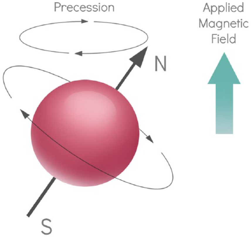
Precession. The alignment of nuclei with an applied magnetic field is not stagnant. Nuclei wobble or ‘precess’ around the direction of the magnetic field. This motion is similar to how a spinning top would wobble/precess around the vertical gravitational field. (N = North, S = South.)

The magnetic field of the protons that are in parallel alignment with the main magnetic field is canceled by the almost equal number of protons that are in antiparallel alignment. At thermal equilibrium, there is always a small excess of protons that are in parallel alignment. The collective magnetic strength (called M₀) of this small excess of protons forms the basis for signal generation.

Precessing protons can receive and exchange energy. To get signal from the leg, a transmit coil generates a radio frequency (RF) ‘excitation’ pulse that delivers energy to the protons. The energy can only be transferred if the RF pulse is tuned to the same frequency as the proton magnetization’s precession frequency (‘resonance’). At thermal equilibrium, the M₀ is aligned in the direction of the main magnetic field in the MRI scanner (i.e. the axis from head to foot). As protons absorb energy, M₀ is shifted away from that direction into a transverse plane creating a M_xy. This M_xy continues to precess and this wobbling magnetization produces a voltage in a wire that can be measured.

This process of generating signal is summarized in Figure 2.

Figure 2.

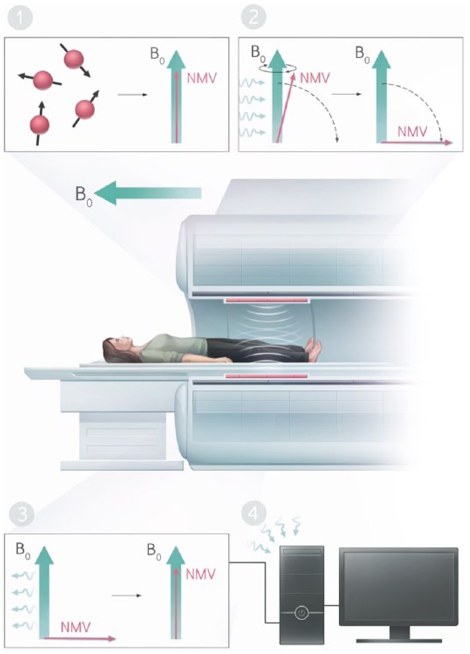
Generating signal. (1) The ‘spins’ associated with protons of the body have random orientations at baseline and their orientation will align with the main magnetic field (B₀) when the body enters the field, summing to a net magnetization vector (NMV) aligned with the field. At equilibrium, the amplitude of this magnetization is M₀. (2) A radio frequency pulse delivers energy to the spins which tips the direction of magnetization away from the main magnetic field. (3) The oscillation of the transverse magnetization induces a voltage signal in a receive coil, modulated at the same radio frequency. (4) The computer processes the radio frequency signals from the coil to create an image.

T1 and T2

The energy gained by the protons is slowly lost and the protons gradually relax back to their thermal equilibrium. This relaxation happens via two mostly independent processes dictated by T1 and T2 values. Consider the contributions from all of the imaged protons in a volume to be described by a single net magnetization vector. With RF excitation, the magnetization vector went from aligned with the main field of the magnet (longitudinal), and was tipped to the transverse plane (perpendicular to the main field), and then the vector relaxes back to its original alignment. T1 is a time constant associated with the regrowth of the longitudinal component of the vector (M_z) along the original alignment, associated with return to ‘thermal equilibrium’ (Figure 3).

Figure 3.

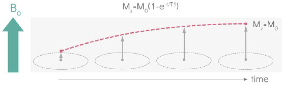
T1 recovery. With radio frequency excitation, the magnetization vector goes from aligned with the main field of the magnet (B₀), and is tipped to the transverse plane (perpendicular to the main field). When the magnetization vector is tipped in the transverse plane, the longitudinal component of the vector (M_z) is 0. When the radio frequency pulse is turned off, the net magnetization vector relaxes back to its original alignment. T1 is a time constant associated with the regrowth of the longitudinal component of the vector (M_z) along the original alignment, associated with return to ‘thermal equilibrium’. At equilibrium, the amplitude of this magnetization is M₀.

The transverse component of the magnetization vectors of all protons precess ‘in phase’ or ‘coherently’. The coherently precessing protons experience slightly different local magnetic fields due to their environment (including from neighboring protons). Their rates of precession vary, leading to accumulation of differences in phase. The resulting loss of coherence leads to decay in the net transverse magnetization (M_xy). The time constant associated with the decay of the transverse component of the magnetization vector is T2 (Figure 4).

Figure 4.

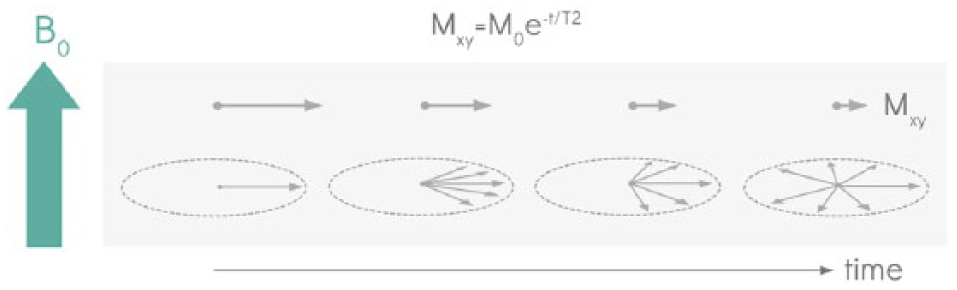
T2 decay. The transverse component of the magnetization vectors of all the protons (which by definition is perpendicular to the main ‘static’ magnetic field (B₀)), precesses ‘in phase’ or ‘coherently’ about that static field at a rate proportional to the strength of the field. Small variations in the field seen by different protons cause their rates of precession to vary, leading to accumulation of differences in phase. The resulting loss of coherence leads to decay in the net transverse magnetization (M_xy). The time constant associated with the decay of the transverse component of the magnetization vector is T2.

Blood and muscle have different T1 and T2 time constants. The image can be acquired at a specific time after the RF pulse to maximize the contrast between tissues based on their different T2s. The time between the RF excitation pulse and the data acquisition is called the ‘echo time’ (TE). The time between RF pulses can also be selected to manipulate how much T1 contrast the image shows. The time between RF pulses is called the repetition time (TR). With the appropriate timing parameters, images from any sequence can be T1-weighted (optimum TR selected for maximum T1 contrast; Figure 5) or T2-weighted (optimum TE selected for maximum T2 contrast; Figure 6).

Figure 5.

Repetition time selection for optimal T1 contrast. Repetition time (TR) refers to the time between successive radio frequency excitation pulses. When the TR is short, the longitudinal component of the magnetic vector (M_z) cannot fully recover to equilibrium (M₀); tissues with short T1 will recover more of M_z compared to tissues with long T1. If the TR is long enough, M_z for all tissues will fully recover, and therefore the contrast between the tissues will be minimal. The TR can be selected to optimize T1 contrast to produce T1-weighted images.

Figure 6.

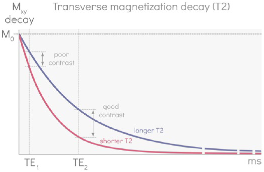
Echo time selection for optimal T2-weighted contrast. The echo time (TE) refers to the time between a radio frequency pulse and when the data are acquired. If the data are acquired too soon after the RF pulse, magnetization from different tissues will not have much time to lose coherence and the transverse component of the magnetization vector (M_xy) remains high. By waiting to acquire the data (longer TE), transverse magnetization for tissues with short T2 will decay faster and therefore M_xy will be lower than tissues with longer T2. The TE can be selected to optimize T2 contrast to produce T2-weighted images.

Impact of exogenous contrast agents

Exogenous contrast used in CT/X-ray imaging involves imaging contrast agents with high atomic numbers (typically iodine and barium) to better absorb X-rays and thus attenuate the signal. MRI, on the other hand, does not image the contrast agent itself but instead uses it to manipulate the relaxation times of structures. The most commonly used MRI contrast agents are gadolinium based. Gadolinium has a unique structure with unpaired electrons such that if it is injected intravenously and comes in close proximity (< 3 angstroms) to the protons of the blood, a quantum mechanical interaction will occur. During this interaction, energy from the fluctuation in local magnetic fields associated with the motion of gadolinium alters the magnetization associated with the proton, accelerating the proton T1 relaxation and making T1 much shorter. Regions of high gadolinium concentration appear very bright on T1-weighted images because there is more contrast between the T1s of the muscle and gadolinium-enhanced blood. While gadolinium based agents continue to play the main role, ferumoxytol has also been studied but is currently not approved by the US Food and Drug Administration for use as a contrast agent.⁴

Acquisition pulse sequences

As stated earlier, the frequency describing how quickly the magnetization in the transverse plane precesses is proportional to the magnetic field. An additional magnetic gradient (G_z) can be applied to change the frequency of how fast the magnetization precesses at specific locations along an axis. Since the RF pulse will only deliver energy to protons that are precessing at the same frequency, the RF pulse can be tuned to ‘select’ a specific location/slice (Figure 7). Only those protons will generate signal.

Figure 7.

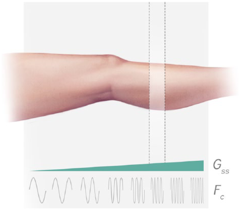
Slice selection. An additional magnetic gradient (G_ss = slice selective gradient) can be applied to change the frequency (F_c) of how fast the magnetization precesses at specific locations along an axis. Since the radio frequency pulse will only deliver energy to protons that are precessing at the same frequencies as the oscillations of the magnetic field in the pulse, the radio frequency pulse can be tuned to ‘select’ a specific location/slice.

Magnetic gradients are applied in the other two axes (G_x and G_y) to similarly spatially encode the signal based on differences in signal modulation frequencies corresponding to different spatial locations. For a more in-depth discussion of spatial encoding, see McRobbie et al.⁵ A basic pulse sequence involves three steps (Figure 8):

Step 1: RF pulse tuned to select a specific slice (z-direction)

Step 2: Magnetic gradient applied in the y-direction (‘phase encoding’)

Step 3: Magnetic gradient applied in the x-direction (‘frequency encoding’) and acquiring a single line of data.

Figure 8.

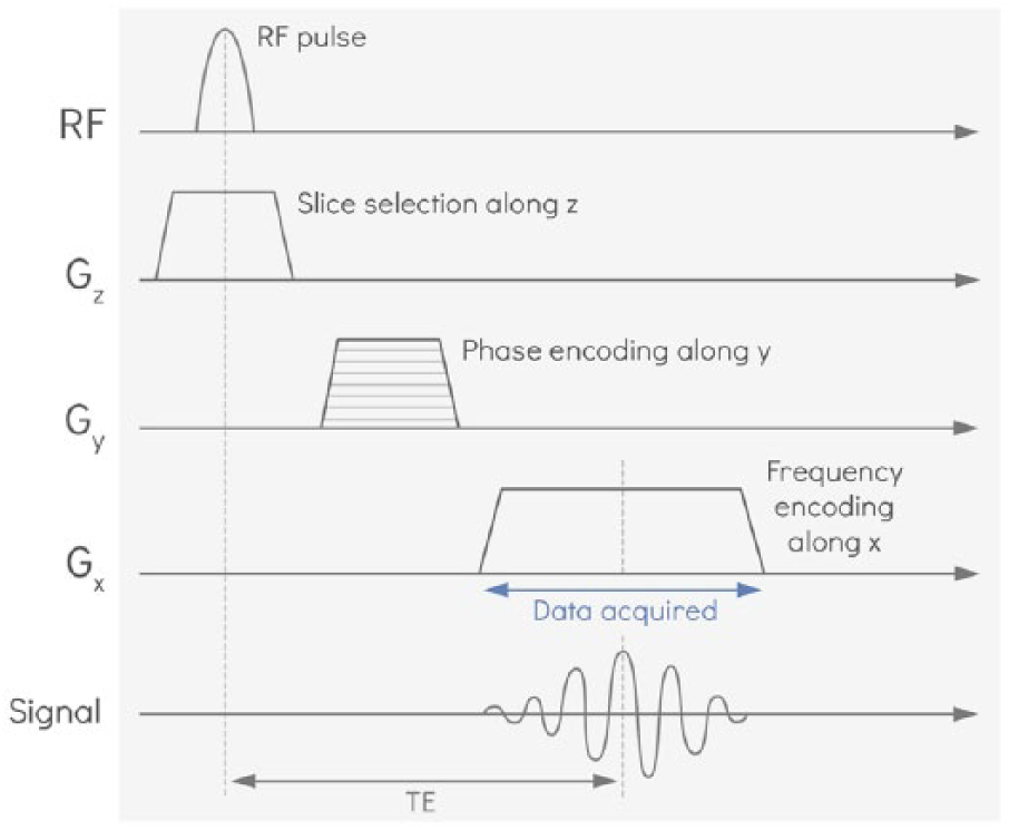
Anatomy of a basic pulse sequence. A radio frequency pulse is tuned to select a specific slice (z-direction). For encoding spatial position within the resulting image plane, a magnetic gradient is applied in the y-direction (‘phase encoding’) and then a magnetic gradient is applied in the x-direction (‘frequency encoding’) while a single line of data is acquired. The echo time (TE) is the time between the radio frequency pulse and when the data are acquired. In subsequent acquisitions, the phase encoding gradient is incremented until enough lines of data (typically around 200 lines) have been acquired to fully map the 2D plane. With an additional nested loop of phase encoding in z, this can be extended to a 3D volume.

This process repeats over again until the entire image slice is acquired.

Using MRI pulse sequences to evaluate peripheral arterial lesion characteristics

Lesion length: Lumen assessment with bright blood imaging

Lesion length can be evaluated with bright blood MRI sequences, which are generated with a specific class of MRI pulse sequences called ‘gradient echo’ sequences. Gradient echo sequences can produce bright blood angiograms both with and without the use of exogenous contrast agents. When a magnetic gradient is applied, protons at different spatial locations will precess at different frequencies. When the magnetic field experienced by a proton fluctuates due to the effects of neighboring protons, it modulates the precession frequency introducing phase shifts among a group of protons, leading to loss of coherence in associated magnetization vectors, causing signal to decay (T2 relaxation; Figure 4). In addition, signal decays due to protons experiencing varying magnetic fields associated with the imposed gradient. To generate a gradient echo, equal and opposite gradients in magnetic fields are applied for the same period of time to reverse the gradient-driven signal decay. First, a negative gradient is applied so that the protons’ magnetization vectors precess at different frequencies, lose coherence and the signal decays. When an equal and opposite gradient is applied, the magnetization vectors’ relative precession direction will be reversed so that their relative phases re-align and they add constructively, recovering the associated signal. A pictoral representation of this process is provided in Figure 9. The recovered signal is referred to as an ‘echo’ and the image is acquired at the peak of this ‘echo’.

Figure 9.

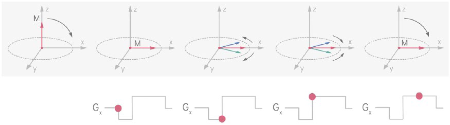
Gradient echo formation. A negative gradient (G_x) is applied so that the protons’ magnetization vectors at different spatial locations precess at different frequencies and lose coherence so that the net signal decays. An equal and opposite gradient is applied to reverse the magnetization vectors’ relative precession direction. Their relative phases re-align and they add constructively, recovering the associated signal. The recovered signal is referred to as a ‘gradient echo’.

Non-contrast-enhanced MRA

The ‘2D time-of-flight’ sequence has traditionally been used to generate bright blood MR angiograms without the use of exogenous contrast agents. It is a type of gradient echo sequence but uses ‘magnetic saturation’ to establish contrast between static and flowing protons. Before the image is actually acquired, a series of repetitive RF pulses are applied to a specific slice, such that the longitudinal magnetization does not recover before the next RF pulse. This ‘saturates’ the stationary tissue and decreases the signal from it. When the image is acquired, fresh blood that subsequently flows into that imaging slice has not been subjected to the magnetic saturation, and thus has higher signal compared to the stationary tissue. This effect is known as ‘flow-related enhancement’ and produces bright blood angiograms. This technique can be used to locate peripheral arterial lesions as darker regions within the blood vessels are associated with a lack of flowing blood, and facilitate measurement of the length of lesions. Time-of-flight sequences can image slower flowing blood than DSA and up to 20% of tibial vessels seen with time-of-flight sequences are not detected with DSA.⁶

Pitfalls and limitations – Time-of-flight imaging for PAD is no longer routinely used in clinical practice because it has several limitations.⁷ The saturation of flowing blood depends on multiple parameters including blood flow velocity, blood flow direction, slice thickness, and repetition time. Blood flow with optimal velocity, perpendicular to the imaging slice, imaged with multiple thin slices and long repetition times, will produce the most signal. These requirements introduce multiple challenges. In large vessels with high-velocity blood, the frequency of the flowing spins is altered as the spatial-encoding gradients are applied. As a result, spins within the same voxel become out of phase with each other and the total signal from that voxel is diminished. This phenomenon is referred to as ‘intra-voxel dephasing’. Small vessels with slow flow also pose challenges. When slow-flowing blood gets partially saturated, its signal diminishes and vessels can appear to have ‘pseudostenoses’⁷ (Figure 10). This is a particular problem in occlusive tibial vessels with slow blood flow that varies with different phases of the cardiac cycle. Thinner slices improve sensitivity to slow-flowing blood but increase scan time to cover the same volume (more slices per volume). Longer acquisition times also mean that patients are more likely to move within the scan time and patient motion significantly compromises image quality. The 2D time-of-flight techniques have limited spatial resolution compared with 3D techniques, but 3D techniques are more prone to problems with blood vessel saturation within an imaging section. The 3D techniques also have much longer acquisition times and are considered to be impractical for lower extremity imaging due to the large area of anatomic coverage required. Also, they are all flow-dependent techniques that make it challenging to evaluate distal occlusive tibial vessels with very slow flow. Many newer sequences address some of these challenges and are further detailed in other reviews.⁸

Figure 10.

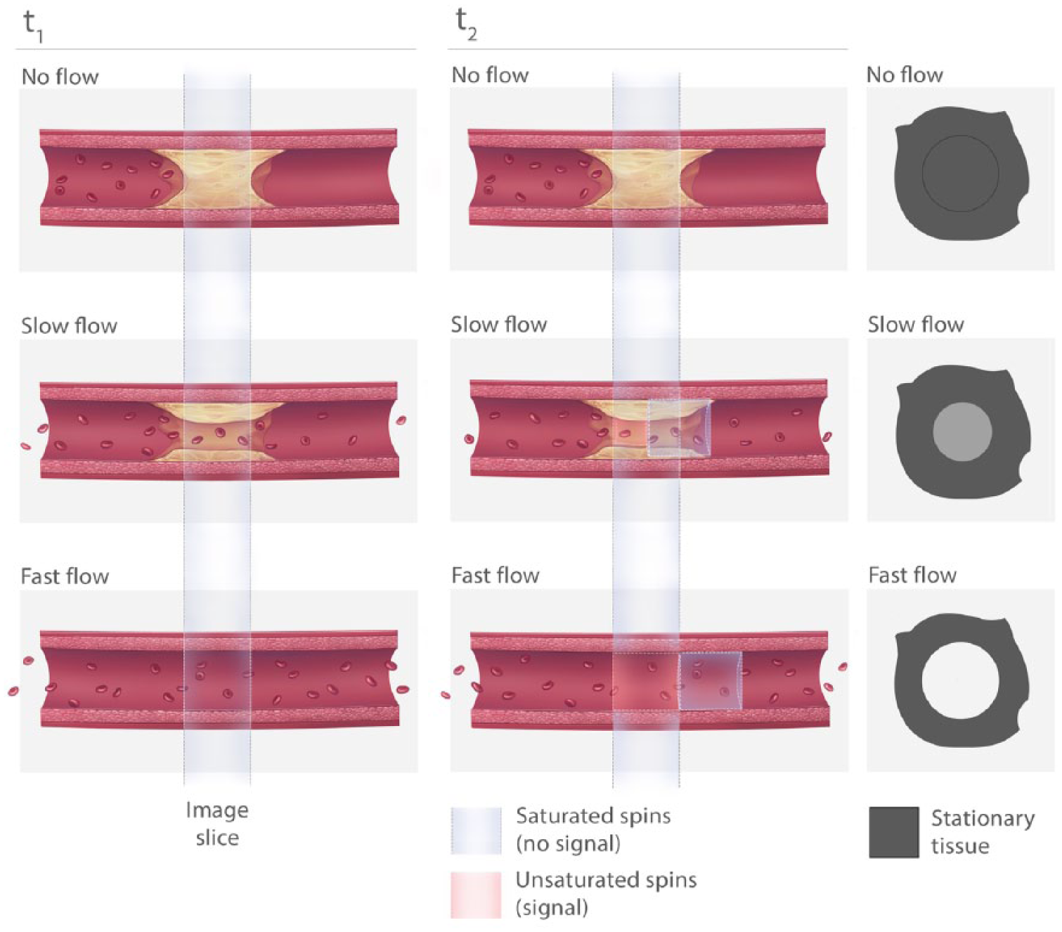
Flow enhancement in time-of-flight sequences. When there is a complete occlusion, both the lesion and the vessel wall are stationary. Their signals are saturated by a series of repetitive RF pulses, limiting recovery between pulses. When there is slow flow, some of the blood (that is in the slice for a long enough time to experience multiple radio frequency pulses) may get partially saturated, which diminishes the signal intensity of blood in the imaging slice. To get the most signal from blood, the flow must be fast enough such that the saturated spins wash out of the imaging slice and fresh blood that was not subjected to magnetic saturation by multiple radio frequency pulses washes into the imaging slice.

Contrast-enhanced MRA

Contrast-enhanced MRA sequences remain the mainstay of clinical peripheral MRA. Contrast-enhanced sequences typically result in higher quality images with a better signal-to-noise ratio in a shorter scan time compared with non-contrast-enhanced methods. MR imaging always involves a compromise between signal-to-noise ratio, spatial resolution and scan time. Contrast-enhanced time-resolved MRA techniques are particularly well-suited and use the improved signal-to-noise ratio to address the inherent trade-offs between spatial and temporal resolution.

When MR signals are acquired, the raw data are stored as an array of numbers that represent spatial frequencies in the MR image (‘k-space’). The center of k-space contains information about image contrast and the edges of k-space encode edge definition. Typically, increasing spatial resolution requires sampling more points, which necessitates longer acquisition times. Time-resolved MRA uses ‘view-sharing’ to address these competing constraints. First, an unenhanced image is acquired at full resolution. Then, a contrast bolus is injected and the center of k-space (which contains contrast information) is sampled more often than the periphery. By combining the data from different partial k-space sampling patterns, it is possible to generate a series of time-resolved images at rates of one to two frames per second, while still maintaining adequate spatial resolution.⁹ Time-resolved MRA has a reported specificity of 99% and sensitivity of 85% for evaluating PAD.⁹

Pitfalls and limitations – Contrast-enhanced methods are contraindicated in many PAD patients with renal impairment. Most contrast agents are gadolinium based and are contraindicated in patients with glomerular infiltration rates (GFR) less than 30 mL/min and should be used with caution in patients with a GFR under 60 mL/min.¹⁰ Other agents may be better suited for PAD imaging in the future. Ferumoxytol can be used in patients with renal impairment and is a blood-pool agent with an extended plateau of increased vascular signal compared to extracellular gadolinium based contrast agents.⁴ Contrast-administration timing can be challenging in distal occlusive vessels and the extended plateau of ferumoxytol may be particularly beneficial for these vessel beds.

Degree of stenosis: Wall assessment with black blood imaging

Black blood sequences are well suited to evaluate the vessel wall because they attenuate the signal from blood (again using time-of-flight effects). This enables better visualization of the plaque burden, luminal surface and the lesion causing the stenosis.¹¹ A class of MRI pulse sequences called ‘spin-echo’ sequences produces images with intrinsic black blood contrast. Spin-echoes are created by two successive RF pulses. First, a 90 degree pulse is used to tip the net magnetization vector into the transverse plane for a target slice as discussed earlier. After a period of time, the spins will lose coherence and signal starts to decay. A 180 degree refocusing pulse is then applied, which flips the spins in the same slice such that their associated magnetization vectors come back together forming an ‘echo’ and the signal is acquired at this point. A pictorial representation of this process is shown in Figure 11. Eventually the spins will de-phase once again. Spin-echo sequences produce black blood images because all of the blood that received the first 90 degree pulse washes out of the slice before the 180 degree refocusing pulse and the resulting image has a signal void where the originally excited blood has washed out. Plaque burden measurements with black blood MRI sequences have high reproducibility and reliability (intra-observer intraclass correlation R = 0.997, inter-observer R = 0.987, and test-retest reproducibility R = 0.996).¹² Plaque burden measurements have also been highly correlated with clinical signs and symptoms, including ankle–brachial indices and walking impairment.¹³

Figure 11.

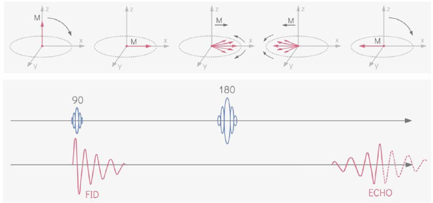
Spin-echo formation. A 90 degree radio frequency pulse tips the net magnetization vector into the transverse plane. The spins will lose coherence and signal starts to decay (free-induction decay; FID). A 180 degree refocusing pulse flips the spins in the same slice such that their associated magnetization vectors come back together. The recovered signal is referred to as a ‘spin-echo’.

Pitfalls and limitations – Similar to bright blood time-of-flight gradient echo sequences, imaging slow-flowing blood with this technique can be challenging because of incomplete washout of the blood through the slice. Spin-echo sequences also suffer from long acquisition times, which limit anatomic coverage and spatial resolution, and exacerbate artifacts from patient motion.

Run-off assessment: Flow-independent imaging with steady state free precession sequences

The success of PAD revascularization procedures depends on adequate run-off.^1,14,15 It is challenging to image run-off vessels with current methods because there must be sufficient flow to detect blood within vessels (e.g. duplex ultrasound or most non-contrast-enhanced MRA) or there must be sufficient flow to opacify vessels with contrast media (e.g. digital subtraction angiography, CTA or contrast-enhanced MRA). MRI has a unique advantage because it can image slow-flowing or even stagnant blood and produce flow-independent bright blood angiograms using steady state free precession (SSFP) sequences. These sequences use the intrinsic T2/T1 contrast between blood and surrounding tissues and therefore do not rely on flow-enhancement required with bright blood time-of-flight gradient echo sequences and black blood spin-echo sequences. This may prove to be particularly advantageous to evaluate run-off vessels that can be occult with DSA,⁶ CT angiography¹⁶ and other MRI methods.

Thus far we have discussed RF pulses that tip the net magnetic vector into the transverse plane. In SSFP sequences, the net magnetic vector is tipped with a smaller flip angle (typically 45 degrees) and the TR is selected to be much shorter than T2. The shortened TR not only decreases the total acquisition time of the scan, but also means that the signal does not fully decay and the transverse components of magnetization never fully dephase before the next RF pulse is transmitted. Rapid repetition of RF pulses where all gradient based dephasing is corrected before each pulse, results in recycling transverse magnetization and mixing it with contributions from recovered longitudinal magnetization (M_z) in subsequent acquisitions. This yields a generally stronger signal with contrast affected by both T2 decay and T1 recovery.

The train of repeated RF pulses is transmitted until a ‘steady state’ is achieved where the net magnetization vector remains consistent.

Steady state can only be achieved if:

TR is much shorter than T2 and the remnant transverse magnetization component is either spoiled (i.e. incoherent SSFP) or refocused into the next excitation (i.e. coherent or balanced SSFP).

The phase shifts caused by the gradients in the x, y and z directions must remain constant from cycle to cycle. They are ‘rewound’ in between RF pulses in balanced SSFP sequences.

Field inhomogeneities must be static.

The signal intensity of tissues in SSFP sequences are directly related to the T2/T1 ratio. Solids typically have low T2/T1 (e.g. skeletal muscle = 0.03 at 3T) and liquids have high T2/T1 (e.g. blood = 0.14 at 3T).^17,18 Therefore, blood appears very bright and may even be seen in veins in addition to arteries. Other preparatory pulses are typically used for venous suppression.

Pitfalls and limitations – SSFP sequences for peripheral artery imaging are still under investigation. Recent research is promising and the sensitivity, specificity, negative predictive value, and positive predictive value of SSFP MRA for run-off vessels has been reported (96.4%, 93.0%, 98.5%, and 84.1%, respectively).¹⁹ The safety of SSFP sequences may be a limitation to widespread clinical use. These sequences rely on RF pulses repeated with short TR before the transverse magnetization disappears. The repeated RF pulses can deposit substantial energy, which can heat the tissue and raise safety concerns. Also, since the transverse magnetization is ‘recycled’, any inhomogeneities or variations in the static magnetic field will cause unequal phase accumulation between the RF pulses. Under such circumstances, the refocusing mechanism fails and can result in banding or stripes in the image.

Calcium scoring: Ultrashort echo time sequences

Conventional MRI sequences cannot visualize calcium and this has been a key limitation to using MRI for imaging PAD. Calcium has very short T2 decay times and the signal decays before the data are acquired at conventional TEs. Calcium therefore appears as signal voids on the final image. With improvements in sequence design, magnetic gradient performance and reconstruction techniques, it is now possible to image tissues with ultrashort TE (UTE; typically 0.1–1 ms).^20,21 UTE imaging has the additional advantage of visualizing dense collagen, which cannot be seen on X-ray angiography or clinical CTA. Lesions composed of dense collagen are also difficult to treat percutaneously^20,22,23 and are important to identify. Ultrashort echo time sequences sample data immediately after the RF pulse, before the signal from calcium and collagen decays. Data are acquired while the readout gradient ramps up using non-Cartesian sampling (e.g. radial, spiral or cone trajectories in the data acquisition space called k-space) to enable faster data acquisition to minimize the TE.²⁴ UTE acquisition has primarily been used in musculoskeletal imaging²¹ but cardiovascular applications are being investigated. Figure 12 shows a popliteal chronic total occlusion imaged with both a conventional MRI sequence (fast spin-echo) and UTE imaging, and compares it with high-resolution CT (10 µm × 10 µm × 10 µm). This figure shows high-resolution ex vivo UTE imaging, but it is also feasible to image peripheral vessels in vivo using clinical scanners. Edelman et al. conducted a pilot study using UTE to detect PAD calcifications in iliofemoral arteries²⁵ in seven patients with known calcifications. This group achieved a UTE of 0.07 ms using a clinical scanner and a clinically feasible protocol and validated their technique with CT.²⁵ In a more recent pilot study of 14 PAD patients undergoing infrainguinal endovascular treatment, UTE imaging was used to identify calcified and non-calcified hard lesions that required longer guidewire crossing time and required stenting more often.²⁶ MRI plaque characterization for PAD is still in the early stages of research but may assist in the clinical management of patients in the future.

Figure 12.

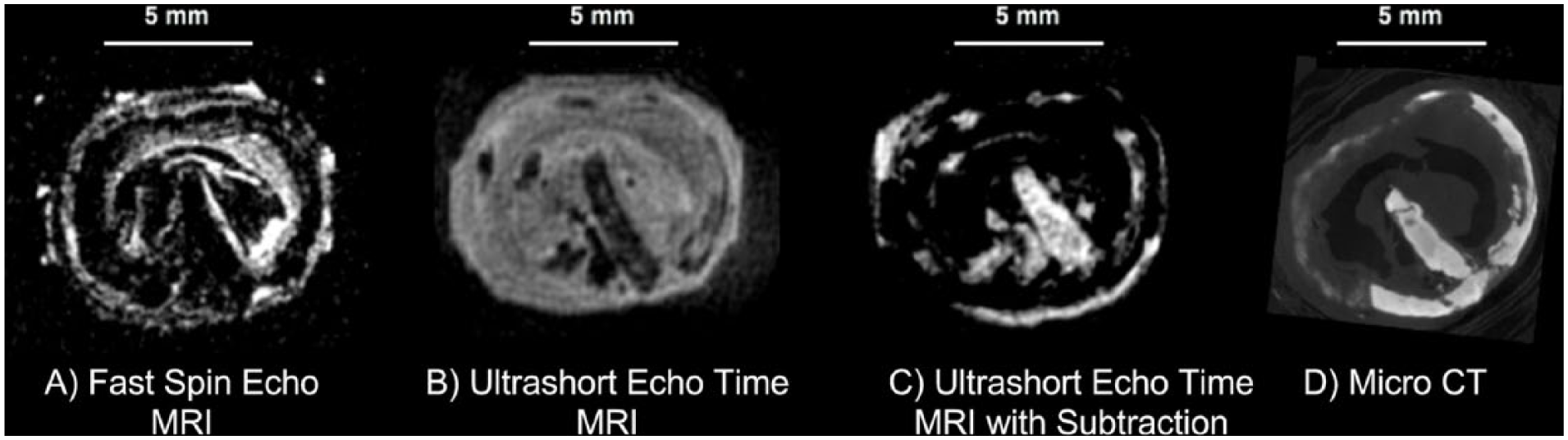
Ex vivo popliteal chronic total occlusion imaged with 7T MRI and microCT. (A) Fast spin-echo sequences and all other conventional sequences cannot visualize calcium or dense collagen because their signals decay too quickly. Areas of the calcium ring and the central calcium nodule appear as signal voids. (B) Ultrashort echo time MRI can visualize tissues with short T2 decay times including calcium and collagen. (C) To highlight tissues with short T2 decay times, images acquired at later echo times can be subtracted from ultrashort echo time images. The popliteal calcium nodule, calcium ring and dense collagen surrounding the nodule appear much more obvious in subtracted images. (D) The microCT image shows calcium but does not visualize dense collagen.

Pitfalls and limitations – Imaging tissues like calcium and collagen is challenging because their signal decays in such a short period of time. The T2 decay rate of most tissues is much longer than the RF excitation pulse duration and the amount of signal decay during the excitation pulse is minimal. However, when the T2-decay rate is very fast, the tissue decays significantly during the RF excitation pulse itself. In such circumstances, the process of the RF pulse tipping the net magnetization vector into the transverse plane will compete with the fast T2-decay, which decreases the magnetization in the transverse plane, making it challenging to acquire the signal. Gradients associated with excitation also extend the delay between excitation and acquisition (increasing TE), so many UTE sequences will avoid using slice-selective gradients (discussed earlier, see Figure 8). Instead, these UTE sequences excite and acquire signal from a large volume, but then must spatially encode that whole volume, which requires long acquisition times. The long acquisition time and quickly decaying signal also make it challenging to image fine detail with high spatial resolution.

Conclusion

PAD is a complex disease process with heterogeneous lesions and challenging anatomic patterns. The vessel wall and complex flow dynamics are key features of this disease process but are difficult to visualize with current imaging. MRI is a powerful imaging modality because the signal and contrast in MR images can be manipulated in countless ways. This review introduced only a few ways that MRI can be used to visualize specific features of PAD. MRI is an incredibly diverse tool that may be useful for clinicians who manage and study PAD. With a basic understanding of how MRI works, clinicians may start to envision the many possibilities of how MRI might improve the management of this growing patient population.

Key points to remember

With the appropriate timing parameters, images from any sequence can be T1-weighted (optimum TR selected for maximum T1 contrast; Figure 5) or T2-weighted (optimum TE selected for maximum T2 contrast; Figure 6).

Unlike CT and X-ray imaging, contrast-enhanced MRI does not involve imaging the contrast agent itself. Contrast agents are used to manipulate the relaxation times of water in tissues. Contrast-enhanced MRA remains the mainstay of MR imaging of peripheral artery disease.

MRI can evaluate lesion length without the use of exogenous contrast using bright blood (gradient-echo) pulse sequences.

Black blood (spin-echo) sequences attenuate blood and can provide cross-sectional images of the vessel wall to facilitate plaque burden and stenosis measurements.

MRI can evaluate slow-flowing or even stagnant blood without exogenous contrast agents with flow-independent SSFP sequences. This may be useful for evaluating distal run-off vessels.

While most MRI sequences cannot visualize calcium, UTE MRI can be used to visualize calcium. This may be useful in calcium scoring and cross-sectional morphology assessment in the future.

MRI offers many benefits and is used clinically for peripheral artery disease imaging. However, in comparison to CT angiography, MRI is limited by long acquisition times, which restricts spatial resolution and anatomic coverage.

Footnotes

Acknowledgements

We thank Hang Yu Lin for illustrating all the figures in this article.

Declaration of conflicting interests

The authors declared no potential conflicts of interest with respect to the research, authorship, and/or publication of this article.

Funding

The authors disclosed receipt of the following financial support for the research, authorship, and/or publication of this article: this work was supported by the Canadian Institutes of Health Research (grant: MOP-126169).

ORCID iD

Trisha L Roy

References

Stoner

Calligaro

Chaer

et al . Reporting standards of the Society for Vascular Surgery for endovascular treatment of chronic lower extremity peripheral artery disease. J Vasc Surg 2016; 64: e1–e21.

Roy

Dueck

Wright

GA.

Peripheral endovascular interventions in the era of precision medicine: Tying wire, drug, and device selection to plaque morphology. J Endovasc Ther 2016; 23: 751–761.

Gerhard-Herman

Member

Gornik

et al . 2016 AHA/ACC Guideline on the management of patients with lower extremity peripheral artery disease: A Report of the American College of Cardiology/American Heart Association Task Force on Clinical Practice Guidelines. J Am Coll Cardiol 2017; 69: e71–e126

Hope

Zhu

et al . Vascular imaging with ferumoxytol as a contrast agent. Am J Roentgenol 2015; 205: W366–W373.

McRobbie

Moore

Graves

et al . Spaced out: Spatial encoding. In: MRI from picture to proton, 3rd edition. Cambridge: Cambridge University Press, 2007, pp.108–136.

Owen

Carpenter

Baum

et al . Magnetic resonance imaging of angiographically occult runoff vessels in peripheral arterial occlusive disease. N Engl J Med 1992; 326: 1577–1581.

Miyazaki

Lee

VS.

Nonenhanced MR angiography. Radiology 2008; 248: 20–43.

Pollak

Kramer

CM.

MRI in lower extremity peripheral artery disease: Recent advancements. Curr Cardiovasc Imaging Rep 2013; 6: 55–60.

Mell

Tefera

Thornton

et al . Clinical utility of time-resolved imaging of contrast kinetics (TRICKS) magnetic resonance angiography for infrageniculate arterial occlusive disease. J Vasc Surg 2007; 45: 543–548.

10.

Hoey

ETD

Ganeshan

Puni

et al . Fresh blood imaging of the peripheral vasculature: An emerging unenhanced MR technique. Am J Roentgenol 2010; 195: 1444–1448.

11.

Balu

Wang

Dong

et al . Current techniques for MR imaging of atherosclerosis. Top Magn Reson Imaging 2009; 20: 203–215.

12.

Isbell

Meyer

Rogers

et al . Reproducibility and reliability of atherosclerotic plaque volume measurements in peripheral artery disease with cardiovascular magnetic resonance. J Cardiovasc Magn Reson 2007; 9: 71–76.

13.

McDermott

Liu

Carr

et al . Superficial femoral artery plaque, the ankle-brachial index, and leg symptoms in peripheral artery disease: The Walking and Leg Circulation Study (WALCS) III. Circ Cardiovasc Imaging 2011; 4: 246–252.

14.

Hiramori

Soga

Tomoi

et al . Impact of runoff grade after endovascular therapy for femoropopliteal lesions. J Vasc Surg 2014; 59: 720–727.

15.

Carpenter

Golden

Barker

et al . The fate of bypass grafts to angiographically occult runoff vessels detected by magnetic resonance angiography. J Vasc Surg 1996; 23: 483–489.

16.

Werncke

Ringe

Von Falck

et al . Diagnostic confidence of run-off CT-angiography as the primary diagnostic imaging modality in patients presenting with acute or chronic peripheral artery disease. PLoS One 2015; 10: 1–17.

17.

Huang

Chen

et al . Are trueFISP images T2/T1-weighted? Magn Reson Med 2002; 48: 684–688.

18.

Stanisz

Odrobina

Pun

et al . T1, T2 relaxation and magnetization transfer in tissue at 3T. Magn Reson Med 2005; 54: 507–512.

19.

Zhang

Fan

Luo

et al . Noncontrast MR angiography (MRA) of infragenual arteries using flow-sensitive dephasing (FSD)-prepared steady-state free precession (SSFP) at 3.0 Tesla: Comparison with contrast-enhanced MRA. J Magn Reson Imaging 2016; 43: 364–372.

20.

Roy

Liu

Shaikh

et al . Puncturing plaques: Relating MRI characteristics of peripheral artery lesions to guidewire puncture forces. J Endovasc Ther 2017; 24: 35–46.

21.

Chang

Chung

CB.

UTE imaging in the musculoskeletal system. J Magn Reson Imaging 2015; 41: 870–883.

22.

Strauss

Osherov

Radhakrishnan

et al . Collagenase total occlusion-1 (CTO-1) trial: A phase I, dose-escalation, safety study. Circulation 2012; 125: 522–528.

23.

Thind

Strauss

BH.

A novel method for the measurement of proximal fibrous cap puncture force in chronic total occlusions: The effect of increasing age. EuroIntervention 2011; 6: 997–1002.

24.

Tyler

Robson

Henkelman

et al . Magnetic resonance imaging with ultrashort TE (UTE) PULSE sequences: Technical considerations. J Magn Reson Imaging 2007; 25: 279–289.

25.

Edelman

Flanagan

Grodzki

et al . Projection MR imaging of peripheral arterial calcifications. Magn Reson Med 2015; 73: 1939–1945.

26.

Roy