Sage Journals: Discover world-class research

Abstract

This study examines the impact of ski tourism on Colorado’s retail marijuana (RMJ) sales, leveraging county-level sales data and ski resort characteristics. Using a two-way fixed effects model, we analyze seasonal variations in RMJ sales across counties with differing ski resort acreages. Our findings indicate that ski resort counties experience significant increases in RMJ sales during peak ski months (December–March), with the most prominent effects observed in counties with the largest ski resorts. The largest ski resort county – Summit County – sees an estimated seasonal increase of $4.35 million in RMJ sales. We estimate the isolated extra-state ski tourism effects and find that while some sales may shift from non-ski counties, the net increase in RMJ sales for the top ski resort counties remains economically significant. Our set of results suggest ski tourism increases Colorado’s retail marijuana sales between $4.5 M and $9.4 M per year.

Keywords

ski resorts Colorado cannabis Z32 L83 R11

Introduction

The landscape of cannabis regulation is changing rapidly across the world. Thailand has reversed earlier liberalization, reinstating strict controls amid concerns about unregulated markets and tourism-driven demand, while Ecuador has recently reduced its tolerance for recreational use. In contrast, Germany and the Czech Republic have introduced controlled legalization or decriminalization measures, and Spain has advanced a regulated framework for medical cannabis. In the United States, cannabis remains illegal at the federal level, but an increasing number of states have enacted or considered liberalization policies. In fact, the US’s tourism leader—Florida, with an estimated 142.9 million visitors in 2024 (VISIT FLORIDA Research, 2025) and travel and tourism accounting for 10% of its 2023 Gross State Product (VISIT FLORIDA Research, 2024)—received 56% approval (it needed 60% to pass) for Florida Amendment 3 which would have legalized the retail sale of cannabis (Smart & Safe Florida, 2022).

Recent work in this journal shows that changes in visitor flows can lead to sectoral shocks (Ortega and Alector Ribeiro, 2025; Sayan and Alkan, 2023) in tourism-related sectors (Abdelsalam et al., 2023), non-tourism industries (Mariolis et al., 2021), and even the shadow economy Kahyalar et al. (2024). Moreover, it has been demonstrated the tourism is linked to vice-related sectors like alcohol (Francioni Kraftchick et al., 2014), sex work (Hall and Ryan, 2005), and gambling (Przybylski et al., 1998; Xu et al., 2025). Yet, to our knowledge, there are no empirical works on the connection between tourism and cannabis consumption.

Though there is a paucity of data on cannabis sales internationally, the US state of Colorado – the first US state to allow retail marijuana sales – has made its sales public data. Moreover, Colorado has a thriving ski resort industry that is, to quote University of Colorado professor Rich Wobbekind, “very much a part of the Colorado brand” (Blevins, 2015). In 2022, Colorado experienced a total of 90 million visits, with tourism accounting for 48% of these trips. The state’s well-documented retail cannabis market and a well-established seasonal tourism industry makes it an ideal setting to study how temporary population inflows influence consumption in regulated leisure markets. While the analysis focuses on Colorado, the mechanisms it reveals—tourism-induced demand shocks, cross-sector spillovers, and seasonal consumption dynamics—are broadly applicable to other regions where tourism and emerging vice industries intersect.

We model Colorado as being “treated” by ski tourists during the ski season (December–March). The influx of visitors represents an exogenous increase in the number of buyers, which increases the demand for retail cannabis (Kang and Lee, 2018; Meehan et al., 2020; Taylor, 2016). We assume supply to be effectively perfectly elastic, as Colorado’s cannabis retail market is highly competitive, with a Herfindahl–Hirschman Index (HHI) of 97.5 (CODOR MED, 2020). Consequently, increases in sales revenue reflect changes in the quantity sold rather than price movements. Because county-level data on tourist arrivals are unavailable, we proxy tourism intensity using the number of ski resort acres. We then employ a two-way fixed-effects event-study model to estimate the effect of ski tourism on cannabis sales during the ski season. Many ski resort employees are local residents who work in other sectors during the off-season (e.g., lift operators who become whitewater rafting guides), suggesting that the primary source of seasonal variation in sales is visitor demand. To address potential bias from within-state tourists, we conduct additional robustness exercises. Our results reveal significant spillovers from ski tourism into a non-tourism sector, consistent with the cross-sectoral linkages identified by Mariolis et al. (2021).

Data

The Colorado Department of Revenue (CODOR) tracks county-level, monthly retail and medical sales and state taxes. This data is publicly available on their website. It would not be surprising if some months, for example February, have lower revenues than others simply because they contain fewer days. Consequently, we analyze the monthly sales divided by the number of days in the month. This panel data set is unbalanced for two reasons. First, the openings and closings of dispensaries are non-uniform so that RMJ sales are initiated in different months, and counties may report zero sales for a month if no dispensary was open. Second, to protect taxpayer privacy under Section 39-21-113 of the Colorado Revised Statues,¹ CODOR does not release (‘NR’) county data unless there are three taxpayers and none represent more than 80% of the total sales. Instead, CODOR releases the sum of all ‘NR’ counties.

County population and the fraction of the population between the ages of 19 and 24 comes from the US Census Bureau’s Population Estimates Program (PEP), which provides annual demographic updates between decennial censuses.

Cannabis consumption patterns may follow tobacco smoking patterns which are influenced by temperature (Chandra and Chaloupka, 2003; Momperousse et al., 2007). So, we include controls for county temperature. This data comes from the National Centers for Environmental Information (NCEI), a division of the National Oceanic and Atmospheric Administration (NOAA). NCEI serves as the US’s official archive for environmental data, managing vast collections of climate, weather, ocean, and geophysical information. We collect average monthly temperature for each county in Colorado using the NCEI’s Climate at a Glance County Mapping system.

To our knowledge, ski resort fundamentals—size, number of lifts, snowfall, etc.—are not reported in a centralized or systematically archived dataset. We therefore scrape these variables from publicly available comparison tables, using current and historical versions to recover a dataset with time-varying resort characteristics. The scraping code and data can be made available upon request.

We remove observations from November 2019 to November 2021 (inclusive) from the data as contaminated by COVID-19 mitigation policy. The 2019-2020 ski season was cut short by Governor Jared Polis’s executive order. During the 2020–2021 ski season, Colorado ski resorts operated under various capacity restrictions to mitigate the spread of COVID-19. These measures included limiting lodging capacity to 25–50% and reducing the number of visitors. By the 2021–2022 season, most outdoor capacity limits had been lifted, allowing normal operations on slopes, chairlifts, and gondolas.

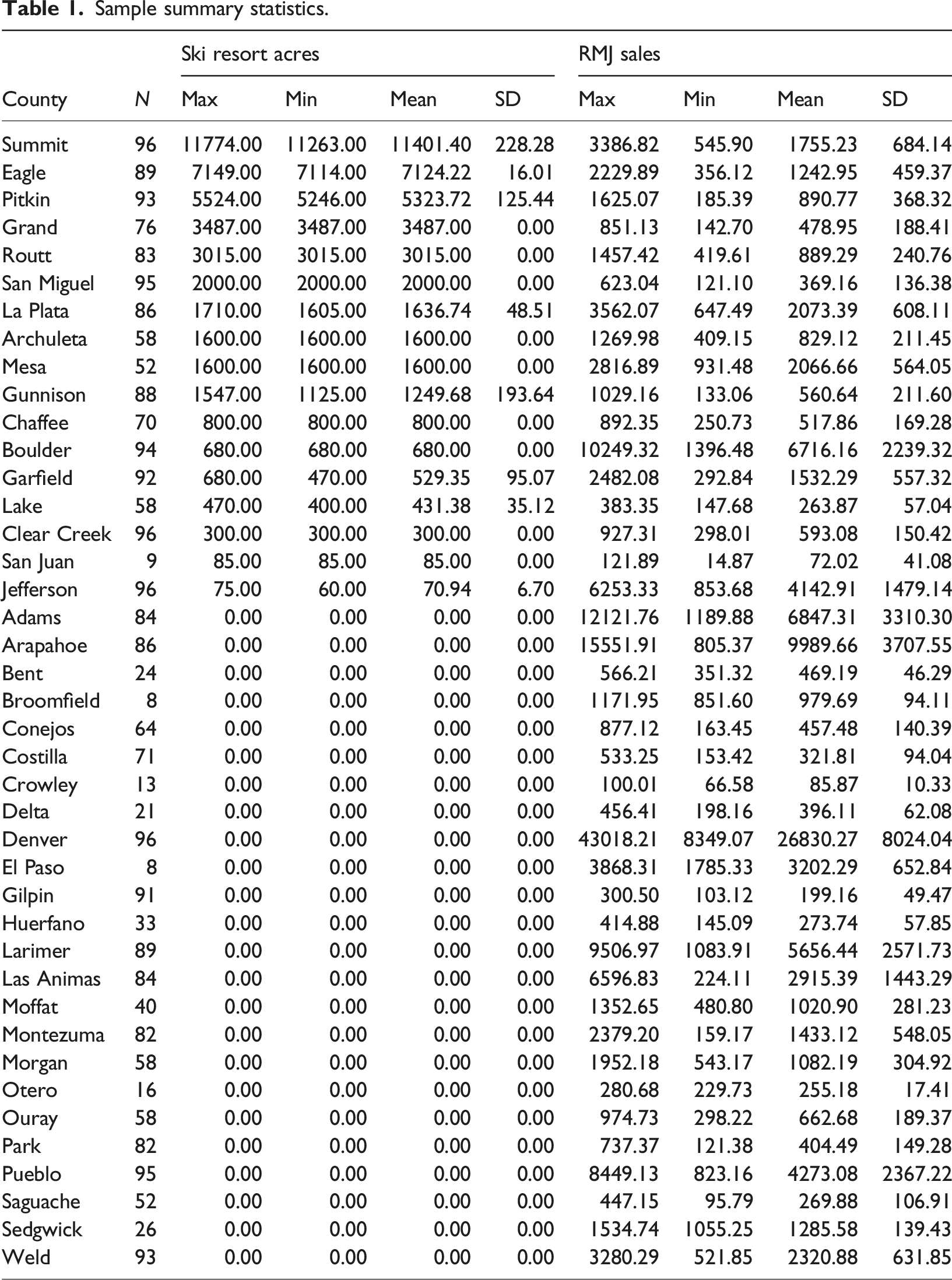
The final sample has 41 of the 64 counties in Colorado. 17 counties have non-zero ski resort acres. The median number of months observed across counties is 82 (mean is 65.9). We observe the maximum value, 96 months, for four counties including Summit (which has five resorts and 11,263 acres, Clear Creek (one resort and 300 acres), Jefferson (one resort and 75 acres), and Denver (no resorts). Summary statistics for ski resort acres and RMJ sales are shown in Table 1.

Table 1.

Sample summary statistics.

		Ski resort acres				RMJ sales
County	N	Max	Min	Mean	SD	Max	Min	Mean	SD
Summit	96	11774.00	11263.00	11401.40	228.28	3386.82	545.90	1755.23	684.14
Eagle	89	7149.00	7114.00	7124.22	16.01	2229.89	356.12	1242.95	459.37
Pitkin	93	5524.00	5246.00	5323.72	125.44	1625.07	185.39	890.77	368.32
Grand	76	3487.00	3487.00	3487.00	0.00	851.13	142.70	478.95	188.41
Routt	83	3015.00	3015.00	3015.00	0.00	1457.42	419.61	889.29	240.76
San Miguel	95	2000.00	2000.00	2000.00	0.00	623.04	121.10	369.16	136.38
La Plata	86	1710.00	1605.00	1636.74	48.51	3562.07	647.49	2073.39	608.11
Archuleta	58	1600.00	1600.00	1600.00	0.00	1269.98	409.15	829.12	211.45
Mesa	52	1600.00	1600.00	1600.00	0.00	2816.89	931.48	2066.66	564.05
Gunnison	88	1547.00	1125.00	1249.68	193.64	1029.16	133.06	560.64	211.60
Chaffee	70	800.00	800.00	800.00	0.00	892.35	250.73	517.86	169.28
Boulder	94	680.00	680.00	680.00	0.00	10249.32	1396.48	6716.16	2239.32
Garfield	92	680.00	470.00	529.35	95.07	2482.08	292.84	1532.29	557.32
Lake	58	470.00	400.00	431.38	35.12	383.35	147.68	263.87	57.04
Clear Creek	96	300.00	300.00	300.00	0.00	927.31	298.01	593.08	150.42
San Juan	9	85.00	85.00	85.00	0.00	121.89	14.87	72.02	41.08
Jefferson	96	75.00	60.00	70.94	6.70	6253.33	853.68	4142.91	1479.14
Adams	84	0.00	0.00	0.00	0.00	12121.76	1189.88	6847.31	3310.30
Arapahoe	86	0.00	0.00	0.00	0.00	15551.91	805.37	9989.66	3707.55
Bent	24	0.00	0.00	0.00	0.00	566.21	351.32	469.19	46.29
Broomfield	8	0.00	0.00	0.00	0.00	1171.95	851.60	979.69	94.11
Conejos	64	0.00	0.00	0.00	0.00	877.12	163.45	457.48	140.39
Costilla	71	0.00	0.00	0.00	0.00	533.25	153.42	321.81	94.04
Crowley	13	0.00	0.00	0.00	0.00	100.01	66.58	85.87	10.33
Delta	21	0.00	0.00	0.00	0.00	456.41	198.16	396.11	62.08
Denver	96	0.00	0.00	0.00	0.00	43018.21	8349.07	26830.27	8024.04
El Paso	8	0.00	0.00	0.00	0.00	3868.31	1785.33	3202.29	652.84
Gilpin	91	0.00	0.00	0.00	0.00	300.50	103.12	199.16	49.47
Huerfano	33	0.00	0.00	0.00	0.00	414.88	145.09	273.74	57.85
Larimer	89	0.00	0.00	0.00	0.00	9506.97	1083.91	5656.44	2571.73
Las Animas	84	0.00	0.00	0.00	0.00	6596.83	224.11	2915.39	1443.29
Moffat	40	0.00	0.00	0.00	0.00	1352.65	480.80	1020.90	281.23
Montezuma	82	0.00	0.00	0.00	0.00	2379.20	159.17	1433.12	548.05
Morgan	58	0.00	0.00	0.00	0.00	1952.18	543.17	1082.19	304.92
Otero	16	0.00	0.00	0.00	0.00	280.68	229.73	255.18	17.41
Ouray	58	0.00	0.00	0.00	0.00	974.73	298.22	662.68	189.37
Park	82	0.00	0.00	0.00	0.00	737.37	121.38	404.49	149.28
Pueblo	95	0.00	0.00	0.00	0.00	8449.13	823.16	4273.08	2367.22
Saguache	52	0.00	0.00	0.00	0.00	447.15	95.79	269.88	106.91
Sedgwick	26	0.00	0.00	0.00	0.00	1534.74	1055.25	1285.58	139.43
Weld	93	0.00	0.00	0.00	0.00	3280.29	521.85	2320.88	631.85

The geospatial overlap between ski resorts and changes in sales is fundamental to the research question. We investigate whether seasonal changes in county sales are attributable to ski tourists. Though the number of ski tourists is unobservable we proxy for it with the number of acres of ski resorts within a county with good reason as over 30% of Colorado’s ski tourists go to the county with the most ski acres – Summit county (Goldsmith et al., 2001). We show the geospatial distribution of ski resort acres and the deviation of ski season RMJ sales from the mean in Figure 1.

Figure 1.

2023 Ski resort acres and changes from mean of RMJ sales.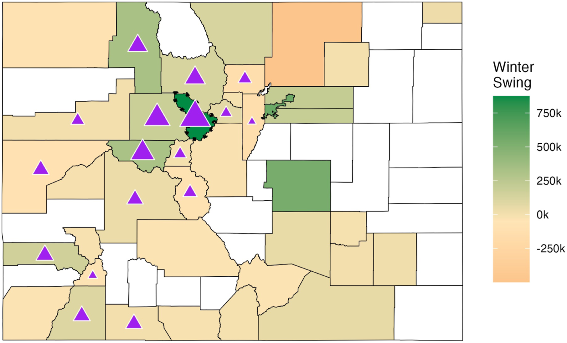

Summit County is in the upper left quadrant of Figure 1 and outlined with a bold dotted line. It has the most ski resort acres in Colorado (as indicated with the largest purple triangle, and also has the largest change in monthly sales in the winter at $873 per day. Eagle County, just west of Summit, is home to the largest ski area in Colorado, Vail, and swings by $183 per day. Just south of Eagle is Pitkin County, home of Aspen ski areas, with a swing of $318 per day.

Empirical approach

Our empirical approach is a reduced-form, two-way fixed effects (TWFE) event study, conceptually related to the canonical difference-in-differences framework. However, we do not aim to identify causal effects. Instead, we make four working assumptions: (1) Colorado counties receive tourists in December–March, (2) the amount of tourists is positively (or at least not inversely) related to the amount of ski resort acres,² (3) RMJ prices do not increase and exhibit limited geographic dispersion (CODOR MED, 2020) so that increases in sales are driven by increases in quantities. Essentially, we assume a basic supply and demand framework for retail cannabis, with very elastic supply, so that changes in sales are driven by changes in demand. We proxy for changes in the (ski season) number of consumers with ski resort acres and allow other potential demand shifters to be absorbed by fixed effects. Under these assumptions, we formulate a reduced-form event study specification to estimate how monthly RMJ sales deviate from annual means across counties with different levels of ski resort intensity. The TWFE design allows us to net out permanent county characteristics and statewide time trends, attributing remaining seasonal variation to localized shifts in consumer volume—primarily driven by tourism. Rather than recovering a structural parameter, our goal is to flexibly characterize the seasonal profile of cannabis demand and how it varies with exposure to ski-driven tourism. The estimating equation follows directly from a simple consumer demand framework, which we outline formally in Appendix A.

A potential concern is that counties with major ski resorts may differ systematically from other counties in ways that also affect RMJ sales, such as population, income, or attitudes toward cannabis. We address this by including county fixed effects, which absorb all time-invariant differences across counties, and time fixed effects, which absorb statewide shocks and common seasonal trends. Our identifying variation therefore comes from within-county changes in sales over time, specifically the interaction between calendar month indicators and cross-sectional differences in ski resort infrastructure. By relying on the event-study form of the TWFE model, we avoid imposing a binary treatment assumption and instead estimate the full monthly sales trajectory across counties with differing levels of ski activity.

Our model is as follows:

Y_{imy} = μ_{i} + ν_{y} + ϵ_{imy} + \sum_{m \in A p r - O c t} α_{m} \cdot D_{m} \cdot S_{imy} + \sum_{m \in D e c - M a r} α_{m} \cdot D_{m} \cdot S_{i m} + X β

(1)where Y_imy is daily average RMJ sales – month sales divided by the number of days in the month – for county i in month m and year y. μ_i and ν_y are county- and year-fixed effects; the clustered standard error is ϵ_imy. D_m indicates whether the observation is in calendar month m. X is a matrix of controls including population, the fraction of the population between 18 and 24, the number of weekend days in month m, monthly temperature, and other covariates on ski resorts (reported average snow, number of runs, vertical feet, number of lifts, peak elevation, and base elevation).³

S_imy is first the amount of ski resort acres in county i in month m and year y. We interpret α_m as the change in per acre daily average sales for a month relative to November. We then subset to counties with ski acres and use S_imy to indicate membership in the Top 1, Top 3, Top 7, or Top 17 (all) counties by number of ski resort acres. This collapses S_imy to S_i as rank does not change. In this specification, we interpret α_m as the change in daily average sales for a month relative to November relative to ski counties that are not the top ranking.

We use the levels of daily RMJ sales, rather than logarithms, for three reasons. First, residents and policymakers are likely more interested in the dollar value which is straightforward in the level specification. Second, tourism-driven shocks to RMJ are not necessarily proportional to county population, which is the main driver of baseline sales. Third, a logged dependent variable may allay concerns of heteroskedasticity; however, county fixed effects absorb persistent differences in scale, and we report robust standard errors clustered at the county level, which are valid under arbitrary forms of heteroskedasticity and serial correlation. Fourth, recent work shows that log-transforming the dependent variable in a difference-in-differences framework can yield treatment effects that differ—even in sign—from those estimated in levels, particularly when baseline outcomes differ across groups (McConnell, 2024).

County ski resort rank is time-invariant and ski resort acres is effectively time-invariant (see Table 1) within counties over our sample period. As standalone regressors, both these variables would be subsumed by county fixed-effects while estimating equation (1). However, these variables are interacted with calendar month dummies and these interaction are time-varying. This allows us to estimate how seasonal variation in RMJ sales differs across counties with different levels of ski resort intensity and group membership. Therefore, all included covariates are identifiable within the fixed effects framework and our coefficients capture seasonal heterogeneity rather than static differences across counties.

Computations were performed in the R environment (R Core Team, 2024) using the fixest (Bergé, 2018) and boot (Canty and Ripley, 2024) packages. The tidyverse (Wickham et al., 2019) package was used for data wrangling and also, with the tigris package (Walker, 2024), for producing figures. The reproducibility file relies on the here package (Müller, 2020).

Results

We begin with the estimation results of equation (1) with S_imy as the amount of ski resort acres in county i in month m and year y. We interpret α_m as the change in per acre daily average sales for a month relative to November and show the estimates in Figure 2. Counties with zero ski resort acres are the comparison group.

Figure 2.

Effect of ski resort acres on RMJ sales.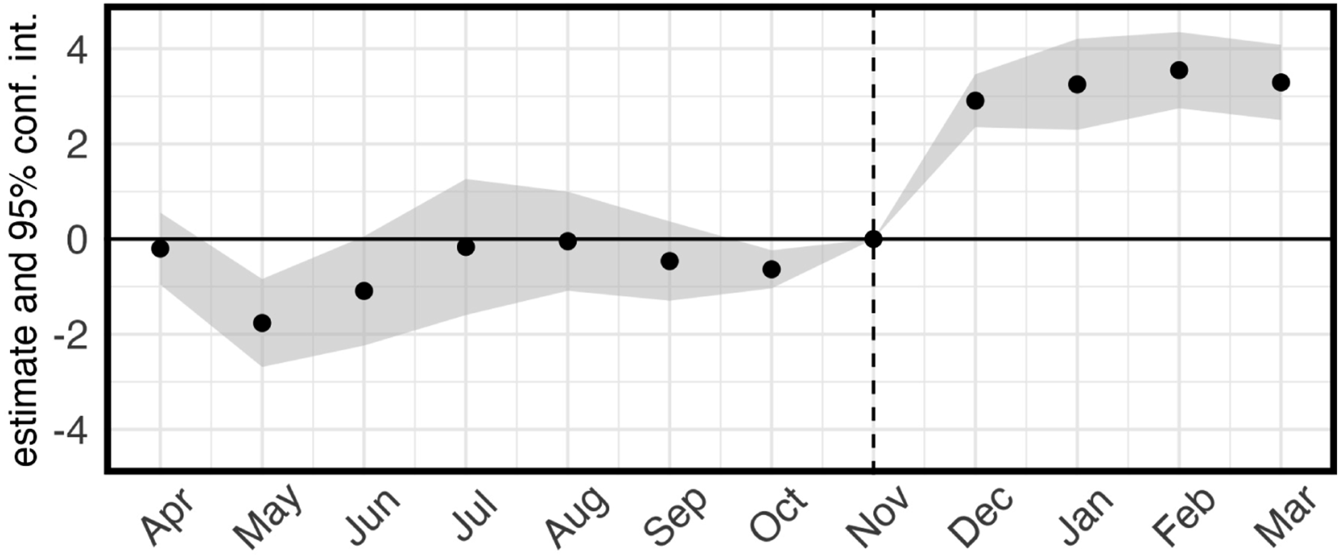

Most, but not all, of the coefficient estimates for the non-ski season months are not statically different than zero. That is, there does not appear to be significant differences in RMJ sales in ski counties versus non-ski counties outside of ski season. There is good evidence of increases in RMJ sales in ski areas during ski season. The estimated effects are: $2.91 \frac{$}{a c r e s \cdot d a y}$ in December, $3.25 \frac{$}{a c r e s \cdot d a y}$ in January, $3.55 \frac{$}{a c r e s \cdot d a y}$ in February, $3.29 \frac{$}{a c r e s \cdot d a y}$ in March; and all are significant at the 99.9% level.

We contextualize this by first multiplying the estimated coefficients against the number of days in each month (ignoring leap years) and summing. This gives $392.38 \frac{$}{a c r e s}$ . Then, we multiply by the number of ski resort acres in the sample: $392.38 \frac{$}{a c r e s} \times 42496 a c r e s = $ 16,674,580$ .

Now, not all ski acres are equally attractive to tourists. For example, Garfield County which has a border on the western edge of Colorado and is the third county down from the northern border in Figure 1, has one ski resort area that is a ‘local’ mountain. It is unlikely that a ski resort acre in Garfield attracts the same amount of tourists as a ski resort acre in Summit County (outlined in Figure 1). Therefore, we suggest the imputed value of $160,634 \frac{$}{d a y}$ is an upper bound of the effect of ski tourists on RMJ sales.

Following the logic that not all ski resort acres are equally attractive, we reconfigure S_imy as an indicator of whether a county is in the Top 1, Top 3, Top 7, or Top 17 (all) by total ski resort acres. As rank does not change over time, S_imy collapse to S_i. We subset to just counties with ski resort acres and and estimate equation (1). The results are shown in Figure 3.

Figure 3.

Effect on RMJ sales by ski resort acres rank.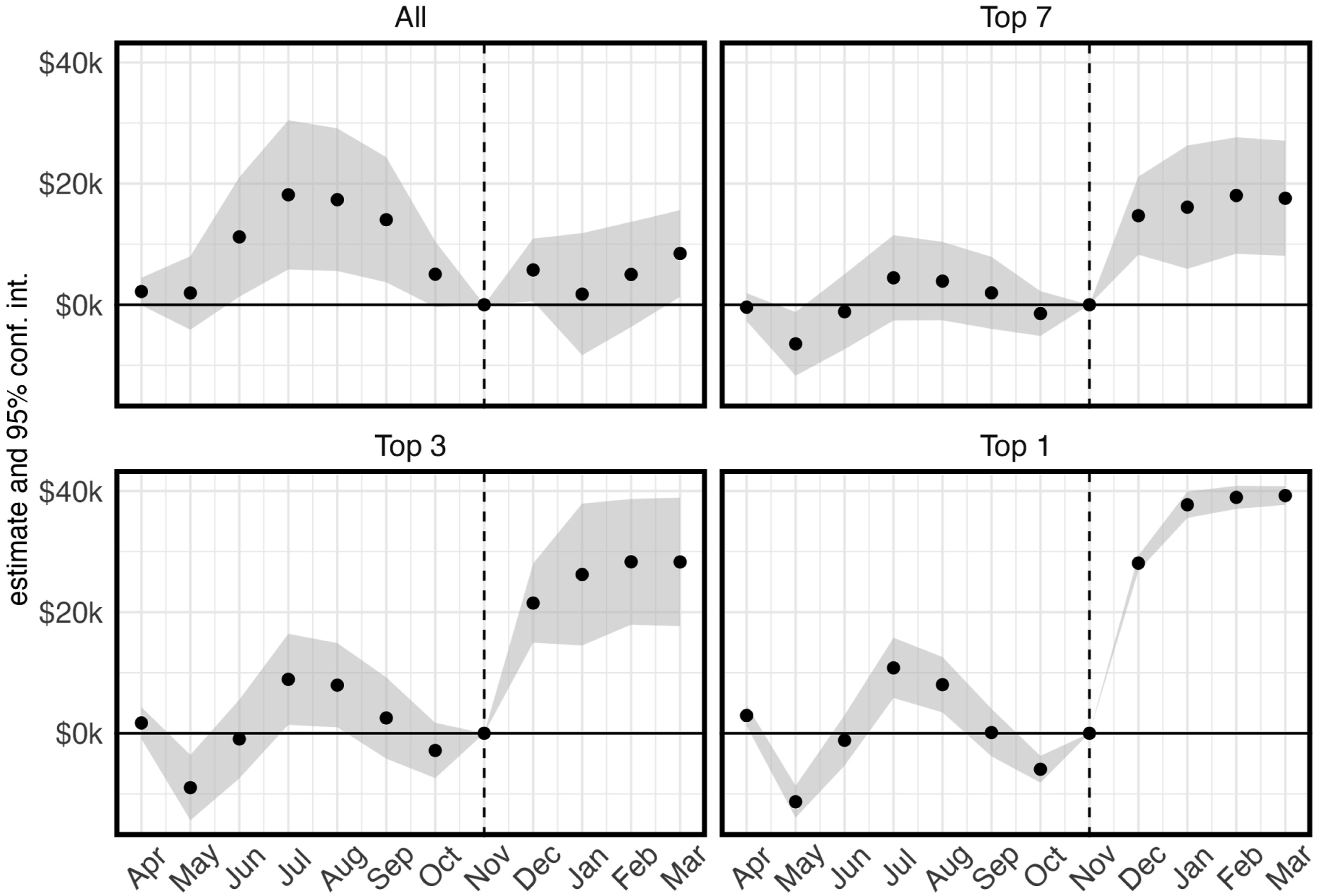

Figure 3 shows the effect of being a top ski resort county in comparison to not top ski resort counties. The upper left panel shows the seasonal pattern of RMJ sales for all ski resort counties with no comparison group. These counties appear to get a statistically significant increase in sales for most of the most of the months (except May) outside of ski season. There no statistically significant effect at the 95% confidence level during ski season.

The upper right panel of Figure 3 shows the estimated effects of the Top 7 ski counties in comparison to counties with less, but still non-zero, ski resort acres. These counties have a different pattern than the full sample of ski resort counties in the upper left panel. With the exception of May, there are no statistically significant effects outside the ski season. This indicates that the control group, counties with less than Top 7 level ski resort acres, is similar to Top 7 counties outside the ski season. However, the Top 7 ski resort counties show statistically significant increases in RMJ sales during the ski season. RMJ sales increase by: $14,704 \frac{$}{d a y}$ in December, $16,105 \frac{$}{d a y}$ in January, $18,306 \frac{$}{d a y}$ in February, and $17,576 \frac{$}{d a y}$ in March. We, again, contextualize this to seasonal effects and find $2,004,974 per Top 7 county, on average. This amounts to a total increase of $14,034,818.

The bottom two panels of Figure 3 show the effect of ski tourism on counties within the Top 3 and Top 1 (Summit) amount of ski resort acres. Both panels show considerable, and statistically significant, non-zero trends outside of ski season. However, the ups and downs are fairly evenly split so that the net pre-trend is zero. Even so, both panels show stronger effects for higher rankings. The lower left panel shows estimated coefficients of: $21,502 \frac{$}{d a y}$ in December, $26,219 \frac{$}{d a y}$ in January, $28,316 \frac{$}{d a y}$ in February, and $28,294 \frac{$}{d a y}$ in March. This is $3,149,368 on average to each Top 3 county for a total increase of $9,448,104. The lower right panel shows estimated coefficients of: $28,093 \frac{$}{d a y}$ in December, $37,733 \frac{$}{d a y}$ in January, $38,956 \frac{$}{d a y}$ in February, and $39,253 \frac{$}{d a y}$ in March. This is $4,348,294 to the Top 1 county – Summit County.

It is likely that some of the increase in sales in ski resort counties is due to Coloradans traveling to those counties and making RMJ purchases there. As seen in the upper row of Figure 3, the ski season increase in RMJ sales is not statistically significant for the full sample though it is for the Top 7. We take this to suggest the Top 7 counties are ‘treated’ by ski tourism and the other counties are not. That is, counties with ‘local mountains’ are not treated alongside counties with no ski areas. We implement this empirically by reconfiguring S_imy to indicate whether a county is in the Top 7 of ski resort acres, again collapsing it to S_i. We then estimate equation (1) with this specification and with the full sample rather than the previously restricted (non-zero ski resort acres) sample. The results are shown in Figure 4.

Figure 4.

Effect on ski resort acres.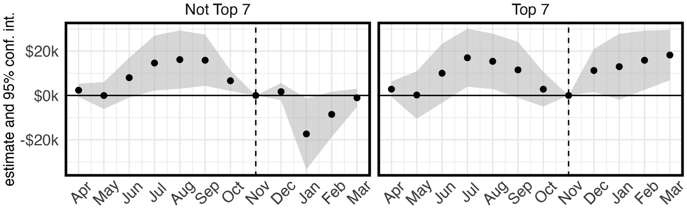

Figure 4 shows that both the Top 7 and the remaining counties in the sample have increases in summer sales. However, there is decline for Not Top 7 – untreated – counties (left panel) that is mostly statistically insignificant. On the other hand, Top 7 – treated – counties have an increase. The decline in sales for untreated counties is plausibly explained, in part, by Colorado residents traveling to Top 7 ski resort counties and making their purchases there.

To investigate this, we estimate the difference (d_m) between the Top estimated coefficients 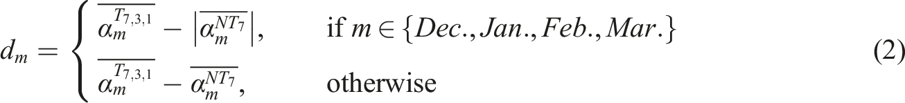$(\bar{α_{m}^{T}})$ and the absolute value of the Not Top $(|\bar{α_{m}^{N T}}|)$ in ski season (m ∈ {Dec., Jan., Feb., Mar.}) to capture the increase in Top net of the what might be a Colorado resident decrease in Not Top 7 ski resort areas (i.e., net of potential intra-state transfers). Outside of ski season, we estimate the difference between the nominal values. This is summarized in equation (2).

d_{m} = \{\begin{cases} \bar{α_{m}^{T_{7,3,1}}} - |\bar{α_{m}^{N T_{7}}}|, & if m \in {D e c ., J a n ., F e b ., M a r .} \\ \bar{α_{m}^{T_{7,3,1}}} - \bar{α_{m}^{N T_{7}}}, & otherwise \end{cases}

(2)

The results of the computation are shown in Figure 5.

Figure 5.

Estimated net effect of ski tourism.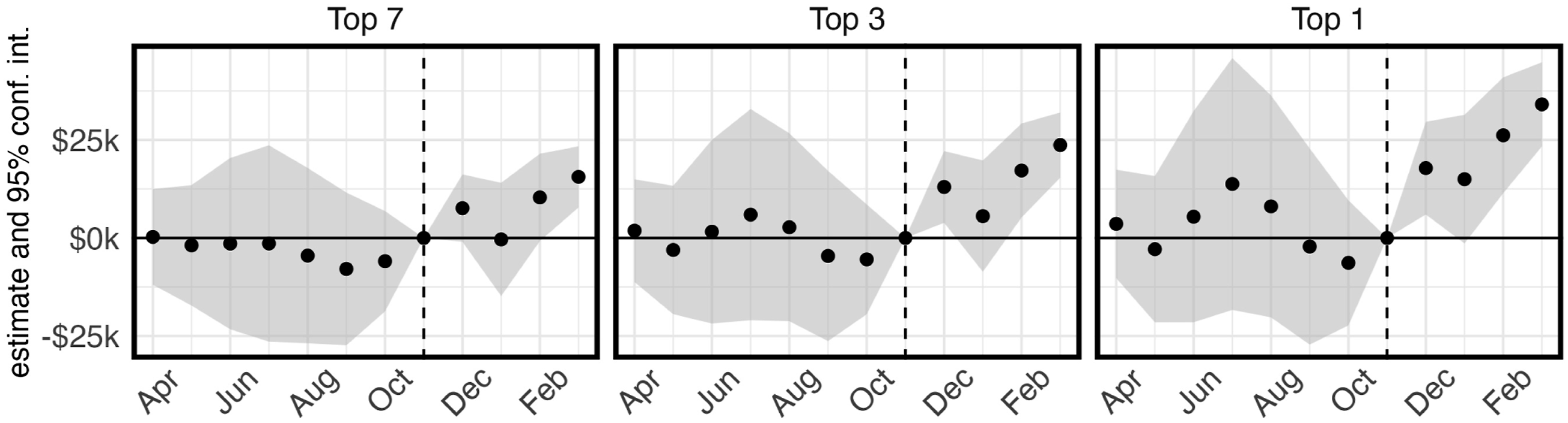

In the left panel of Figure 5, the coefficient estimates for December, January, and February are statistically insignificant, though the point estimates suggest net gains for the Top 7 ski resort counties. However, the coefficient estimate for March is statistically and economically significant at $15,580 \frac{$}{d a y}$ .

The middle panel of Figure 5 shows positive effects for all ski season months and statistically significant effects of: $13,006 \frac{$}{d a y}$ in December, $17,199 \frac{$}{d a y}$ in February, and $23,688 \frac{$}{d a y}$ in March. Excluding January, this amounts to $1,619,088 for the Top 3 summing to $4,857,264.

The right panel shows significant impacts for the Top 1 ski resort county (Summit County): $17,810 \frac{$}{d a y}$ in December, $14,989 \frac{$}{d a y}$ in January, $26,184 \frac{$}{d a y}$ in February $34,066 \frac{$}{d a y}$ in March. This amounts to $2,806,016 for the Top 1 county.

Conclusion

We estimate the effect of ski tourism on Colorado’s retail marijuana sales (RMJ). Using county ski resort acres as a continuous variable implies ski tourism increases RMJ sales by as much as $160,634 \frac{$}{d a y}$ during ski season. However, it may not be that smaller, more ‘local mountain’ areas receive ski tourists. So, we calculate the effect of ski tourism on subsets of ski resort counties based on their ranking by quantity of ski resort acres. We find no effect for the entire sample, but across the ski season each of the Top 7 ski resort counties gain $2,004,974, each of the Top 3 gain $3,149,368, and the Top 1 ski resort county (Summit County) gains $4,348,294.

While these gains to ski resort counties are economically significant, some part may come from Colorado residents (intra-state tourism) who would otherwise make purchases in their home county. We take Not Top 7 ski resort counties, including counties with no ski resorts, as counties unaffected by extra-state tourism and estimate the increase in RMJ sales in ski tourist counties net of intra-state purchase.

That this group may not be completely untreated, and therefore this analysis may not fully eliminate the influence of in-state tourists, is a limitation of the exercise and the results should be taken with a grain of salt. A further limitation of our analysis is the lack of direct evidence on intra-state tourism. Our interpretation—that some residents of Not Top 7 counties travel to ski areas and purchase cannabis—is inferred from the observed winter decline in sales in these counties (see Figure 4), rather than demonstrated with consumer-level data. Finally, we cannot fully distinguish between demand generated by visiting tourists and that arising from migrant workers employed in the ski and hospitality industries. For this reason, it is more accurate to describe the observed patterns as tourism-driven changes in sales.

Regardless, we do not find any economically significant effects for the the Top 7 counties by ski resort acres rank. However, each of the Top 3 counties’ seasonal net increase is $1,619,088 (summing to $4,857,265 for the state) and the Top 1’s increase is $2,806,016. We note that there is a lack of direct evidence of intra-state tourism. Considering the Top 3 ski resort counties as the main source of extra-state effects, ski tourism increase Colorado’s retail marijuana sales are likely between $4.5 M and $9.4 M.

This study is the first to provide an empirical analysis linking tourism intensity to retail cannabis sales. By leveraging seasonal variation in ski tourism, we identify how short-term population inflows create temporary, localized demand shocks that spill over into non-tourism sectors. In doing so, we contribute to the growing literature on cross-sector tourism spillovers and vice-related tourism, offering new evidence that tourism’s economic footprint extends beyond traditional hospitality markets to encompass regulated leisure and retail industries.

Supplemental material

Supplemental Material - Green runs: Colorado cannabis sales during ski season

Supplemental Material for Green runs: Colorado cannabis sales during ski season by Joshua H. Hess, Isabella Bassock in Tourism Economics

Footnotes

ORCID iD

Joshua H. Hess

Funding

The authors received no financial support for the research, authorship, and/or publication of this article.

Declaration of conflicting interests

The author(s) declared no potential conflicts of interest with respect to the research, authorship, and/or publication of this article.

Supplemental material

Supplement material for this article is available online.

Notes

Author biographies

Dr. Joshua H. Hess is a Clinical Associate Professor of Economics at the University of South Carolina’s Darla Moore School of Business. He collected and analyzed the data, authored and edited the manuscript, and is the corresponding author.

Isabella Bassock is an undergraduate economics student at the University of South Carolina’s Darla Moore School of Business. She reviewed the literature and authored and edited the manuscript.

References

Abdelsalam

Faruk Aysan

Cepni

, et al. (2023) The spillover effects of the covid-19 pandemic: which subsectors of tourism have been affected more? Tourism Economics 29(2): 559–567.

Bergé

(2018) Efficient estimation of maximum likelihood models with multiple fixed-effects: the R package FENmlm. CREA Discussion Papers 13.

Blevins

(2015) Skiers’ economic impact in Colorado adds up to $4.8 billion. Denver Post. Available at: https://www.denverpost.com/2015/12/09/skiers-economic-impact-in-colorado-adds-up-to-4-8-billion/.

Canty

Ripley

(2024) Boot: Bootstrap R (S-Plus) Functions. R package version 1.3–31.

Chandra

Chaloupka

(2003) Seasonality in cigarette sales: patterns and implications for tobacco control. Tobacco Control 12(1): 105–107.

CODOR MED (2020) 2020 regulated marijuana market update. Technical report, Colorado Department of Revenue. https://sbg.colorado.gov/sites/sbg/files/2020-Regulated-Marijuana-Market-Update-Final.pdf (accessed 20 May 2025).

Francioni Kraftchick

Byrd

Canziani

, et al. (2014) Understanding beer tourist motivation. Tourism Management Perspectives 12: 41–47.

Goldsmith

Seidl

Weiler

, et al. (2001) Ski-tourism and the economy of summit county, Colorado.

Hall

Ryan

(2005) Sex Tourism: Marginal People and Liminalities. Routledge.

10.

Kahyalar

Seetaram

Fethi

(2024) Tourism and the shadow economy: long-run and short-run implications for resource allocation. Tourism Economics 30(3): 749–766.

11.

Kang

Lee

(2018) Support of marijuana tourism in Colorado: a residents’ perspective using social exchange theory. Journal of Destination Marketing & Management 9: 310–319.

12.

Müller

(2020). Here: A Simpler Way to Find Your Files. https://CRAN.R-project.org/package=here.Rpackageversion1.0.1

13.

Mariolis

Rodousakis

Soklis

(2021) The covid-19 multiplier effects of tourism on the Greek economy. Tourism Economics 27(8): 1848–1855.

14.

McConnell

(2024) Can’t see the forest for the logs: on the perils of using difference-in-differences with a log-dependent variable. Working paper, February 2024. https://hiverev-data.s3.amazonaws.com/media/uploads/1193251363/DiffinDifflogDD.pdf

15.

Meehan

Rusko

Frank Stephenson

(2020) (Pot)heads in beds: the effect of marijuana legalization on hotel occupancy in Colorado and Washington. Journal of Regional Analysis and Policy 50(1): 46–53. https://papers.ssrn.com/sol3/papers.cfm?abstract_id=3776095

16.

Momperousse

Delnevo

Lewis

(2007) Exploring the seasonality of cigarette-smoking behaviour. Tobacco Control 16(1): 69–70.

17.

Ortega

Alector Ribeiro

(2025) An index of the economic dependence on tourism. Tourism Economics 31(3): 426–452.

18.

Przybylski

Felsenstein

Freeman

, et al. (1998) Does gambling complement the tourist industry? Some empirical evidence of import substitution and demand displacement. Tourism Economics 4(3): 213–231.

19.

R Core Team (2024) R: A Language and Environment for Statistical Computing. R Foundation for Statistical Computing. https://www.R-project.org/

20.

Sayan

Alkan

(2023) A novel approach for measurement and decomposition of the economywide costs of shutting down tourism and related service sectors against covid-19. Tourism Economics 29(1): 30–47.

21.

Smart & Safe Florida (2022) Adult personal use of marijuana (initiative 22-05). https://dos.elections.myflorida.com/initiatives/initdetail.asp?account=83475seqnum=2 (accessed 20 May 2025).

22.

Taylor

(2016) Managing recreational marijuana in southwest Colorado. Tourism Review International 20(4): 211–217.

23.

VISIT FLORIDA Research (2024) Florida’s visitor economy normalizes following the pandemic: 2023 economic impact study. Technical report, VISIT FLORIDA, December 2024. https://flgov.com/eog/sites/default/files/shared/2024/12/VisitAccessed:2025-05-20

24.

VISIT FLORIDA Research (2025) Florida visitor estimates and travel industry trend indicators: quarter four 2024. Technical report, VISIT FLORIDA, February 2025. https://flgov.com/eog/sites/default/files/shared/2025/02/Q4Accessed:2025-05-20

25.

Walker

(2024) Tigris: Load Census TIGER/Line Shapefiles. R package version 2.1. https://CRAN.R-project.org/package=tigris

26.

Wickham

Averick

Bryan

, et al. (2019) Welcome to the tidyverse. Journal of Open Source Software 4(43): 1686.

27.

Tian

Zhang

(2025) Tourism, labour migration, and wage inequality: an empirical analysis of Macau’s casino-driven economy. Current Issues in Tourism 1–22.

Supplementary Material

Please find the following supplemental material available below.

For Open Access articles published under a Creative Commons License, all supplemental material carries the same license as the article it is associated with.

For non-Open Access articles published, all supplemental material carries a non-exclusive license, and permission requests for re-use of supplemental material or any part of supplemental material shall be sent directly to the copyright owner as specified in the copyright notice associated with the article.

0.00 MB

0.29 MB