
Abstract
Tourism demand theory postulates that tourists’ incomes, prices in destination countries, and prices in tourists’ countries of origin are key determinants of tourism demand—but must this hold for long-haul travel? We find the answer to be no. By analyzing three international tourist archetypes arriving in New Zealand, a remote island nation, from seven countries, we demonstrate that neither incomes nor prices affect tourism demand in the short run. In the long run, some evidence suggests that tourism demand is income-sensitive; however, it remains insensitive to price changes. We also show that estimates of price elasticities are sensitive to how models are specified and should be interpreted cautiously. The results of this study are broadly relevant to long-haul destinations worldwide.
Introduction
Prices affect tourism demand—evidence abounds in support of this view. However, this may not be true for long-haul travel, which has traditionally been associated with more affluent individuals due to the high costs involved in transportation, accommodation, and other expenses (Boa and McKercher, 2008; Crouch, 1995). Its demand may not be price-sensitive, as those with the wherewithal to afford long-haul travel may not be persuaded or dissuaded by price changes. Furthermore, traditional approaches to modeling prices in tourism research have come under scrutiny (see, e.g., Dogru et al., 2017). The principal reason is this: tourism demand is generally modeled as a function of relative prices, that is, the real exchange rates of a tourist’s country of residence vis-à-vis the destination country and other countries the tourist may have contemplated visiting. The goal of including these real exchange rate series is to examine the own-price and cross-price elasticities of tourism demand. However, due to significant comovement between nominal exchange rates and prices, which form the basis of real exchange rates (Andrieş, Ihnatov and Tiwari, 2016; Ciccarelli and Mojon, 2010; Henriksen et al., 2008), including multiple real exchange rate series may yield unstable and imprecise estimates of price elasticity. Such models warrant reappraisal.
This study has three main objectives. First, it examines the price and income sensitivity of different archetypes of visitors arriving in New Zealand from one neighboring country, Australia, and six distant ones: China, the United States, the United Kingdom, Germany, Japan, and South Korea; these account for 75% of all international visitors arriving in New Zealand and thus present a comprehensive view of the overall international demand for New Zealand tourism; it considers three tourist segments for each country, analyzing 21 segments in total. Second, it demonstrates that price-elasticity estimates are sensitive to model specifications—including exchange rates vis-à-vis multiple countries can generate spurious elasticity estimates and should be interpreted cautiously. Third, it draws a clear distinction between long- and short-run elasticities, showing that tourism demand is more sensitive to income and relative prices in the short run than in the long run.
Why study New Zealand tourism? First, New Zealand is a remote island nation attracting visitors from distant countries: visiting New Zealand entails long-haul travel. 1 Thus, analyzing the demand for New Zealand tourism offers important insights that are broadly relevant to long-haul destinations worldwide. Second, the tourism industry plays a pivotal role in New Zealand's economy—before the onset of the COVID-19 pandemic, it directly employed 8.4% of New Zealand’s workforce, generated significant tax revenues (around US$4 billion in goods and services taxes during the 2018–2019 financial year), and accounted for 20% of New Zealand's total exports of goods and services (Stats NZ, 2020). Even with the importance of international tourism to the New Zealand economy, only one paper, written by Schiff and Becken (2011), has investigated the price and income sensitivity of international demand for New Zealand tourism in detail.
On the whole, however, the tourism literature abounds in the analyses of determinants of tourism demand. Factors such as tourists’ incomes, prices in destination countries and tourists’ countries of residence (Croes and Ridderstaat, 2017; Pham et al., 2017; Schiff and Becken, 2011; Song et al., 2010), oil prices (Becken, 2008; Becken and Lennox, 2012), distance (McKercher, 2018; McKercher and Mark, 2019), terrorism (Adams et al., 2001; Raza and Jawaid, 2013; Thompson, 2011), visa regulations (Li and Song, 2013; OECD, 2014), movies (Li et al., 2017), low-cost carriers (Pulina and Cortés-Jiménez, 2010), cultural similarities (Cheung and Saha, 2015), and marketing initiatives (Ryan, 1991) have been put forth to explain changes in tourism demand. Be that as it may, the first two, that is, income and prices, are widely regarded as the most significant determinants of tourism demand. For example, in a recent study, Muryani et al. (2020) showed that relative prices and tourists’ incomes affected tourism demand in Indonesia. However, there is no consensus on how these factors should be measured. This is especially true for price variables. How can prices be suitably represented in the context of tourism demand? What are the appropriate proxies for the price variables? The answers to these questions are crucial for estimating income and price sensitivities of tourism demand. We address these questions next.
Prices and tourism demand
The distinctions between price variables are drawn along two fundamental dimensions. First, there are differences in how prices are defined. The definitions encompass relative prices (the ratio of prices in the destination country to those in the tourists’ country of residence), substitute prices (the ratio of prices in the destination country to those in countries against which it competes for inbound tourism), and absolute prices (the price level in the destination country). Second, how price indices are constructed varies across studies. These indices can be built using weighted price indices, consumer price indices (CPIs), and tourism-related sub-components of the CPI. The choices as to the combinations across and within these dimensions have important implications for the results, interpretations, and conclusions of the analyses that seek to explain the nexus between prices and tourism demand. These choices warrant scrutiny.
Consider the first dimension. Uysal and Crompton (1984) used relative prices; they defined these as the weighted ratio of prices in the destination country to those in the tourism-generating countries; they derived the weighting by dividing the CPIs in the tourism-generating countries by their currency exchange rates vis-à-vis the destinations country’s currency. Thus, the relative price is simply the real exchange rate (RER) between the destination and the tourism-generating country. However, they also used the nominal exchange rate in conjunction with the RER to estimate various elasticities.
Uysal and Crompton (1985) and Martin and Witt (1988) used both absolute prices (to represent the cost of living in the destination country) and substitute prices (constructed by assigning equal weights to the costs of living in the tourists’ countries of origin, and to the weighted average of the costs of living in the substitute destinations). Owing to how it is constructed, the weighted substitute price index may be used to estimate the price sensitivity of tourism demand; however, it would not allow one to isolate the effects of price levels in competing destinations from those in the tourists’ countries of origin. Furthermore, in both papers, nominal exchange rates were used to convert the living costs in different countries to the currency of the tourists’ countries of origin. This is a sensible approach. After all, tourists evaluate prices in foreign countries in terms of their home currencies. However, despite using exchange-rate-adjusted price levels, a separate nominal exchange rate variable was used to complement the price indices.
Dogru et al. (2017) pointed to multicollinearity in models that use the real and the nominal exchange rates together to explain tourism demand. Expressing concerns regarding the reliability of such models, they estimated four models of tourism demand with different specifications of prices and exchange rates. In the first, they considered both relative and substitute prices, as well as a separate exchange rate variable; in the second, they used exchange-rate-adjusted relative and substitute prices along with the nominal exchange rate; in the third and the fourth models, they used only the exchange-rate-adjusted relative and substitute prices. Notably, relative and substitute prices (with or without exchange rate adjustments) were used in each model. Moreover, these prices were derived with reference to the price level in the destination country, Turkey. Simultaneously using relative and substitute prices, both of which have the same numerator, that is, the price level for Turkey, may generate unreliable estimates. These papers are emblematic of a common approach: they analyze variables constructed from similar constituents, such as price indices and currency exchange rates, which may engender multicollinearity in tourism demand models, as exchange rates tend to co-move.
Among the countries sourcing most of New Zealand’s tourists, Australia, its neighboring country, warrants particular attention: it is the largest importer of New Zealand tourism services. It is also regarded as a substitute destination (Li et al., 2017)—this stands to reason, considering the proximity of the two countries, the stages of economic development, and the distance of the two countries from the rest of the world. However, it bears emphasizing that Australia can also be regarded as a complementary destination. That is to say that travelers from distant countries may consider visiting both countries during their travels to Oceania. In any case, it is reasonable to assume that international demand for the two countries’ tourism services is related. Accordingly, it is important to proceed pragmatically and remain open to the possibility that the two destinations may substitute or complement one another.
In addition, Australia and New Zealand have flexible exchange rate regimes, and both the Australian dollar (AUD) and the New Zealand US dollar (NZD) are regarded as commodity currencies, that is, commodity prices influence their exchange rates. Thus, the RER of a country vis-à-vis Australia is likely to be strongly correlated with its RER relative to New Zealand. In the presence of highly correlated regressors, parameter estimates may be unstable not only in their magnitudes but also in their signs. This has important implications for elasticity estimates: an incorrectly specified model may lead one to conclude that the effect of a variable is positive when the true effect is, in fact, negative; the model may also produce high variances making it challenging to interpret the coefficients.
To be sure, tourists tend to ponder several travel options and compare different destinations before finalizing their travel plans; the ubiquity of information on prices and tourism packages facilitates these comparisons. Thus, there is merit in accounting for prices in different destinations. But herein lies an important trade-off. Is it better to include both kinds of prices and thus potentially compromise the veracity of the estimates? Or is it better to leave out prices in alternate destinations from the model and include only relative prices, thereby not utilizing pertinent information?
Recognizing the importance of understanding the significance of prices in alternate destinations on the one hand and the effects of including highly correlated variables on the other, we estimated two sets of models. The first considered only relative prices, whereas the second comprised both relative prices and prices in alternate destinations. The latter set was derived from the nominal exchange rates of the tourism-importing countries’ currencies vis-à-vis the AUD and their CPIs relative to that of Australia; relative prices were expressed as the exchange-rate-adjusted ratio of prices in New Zealand to those in the tourists’ countries of origin. Both prices are, in essence, RERs vis-à-vis Australia and New Zealand. Using both models allowed us to glean insights into the elasticity estimates and illuminate the effects of using both sets of prices in one model. Even if the presence of highly correlated regressors is unsuitable from an econometric standpoint, robustness checks to see how excluding one or more of such regressors impacts the regression coefficients are warranted because of how common it is in tourism research to consider relative prices and prices in alternate destinations jointly.
Schiff and Becken (2011) noted that stakeholders in the tourism industry have a strong interest in understanding the behaviors of different segments of inbound tourists. This approach provides more granular insights that stakeholders in the tourism industry can utilize to design targeted tourism initiatives—the profiles and proclivities of business travelers are likely to be different from those of holiday travelers. Consequently, we expect their sensitivities to prices and income to be different. With an eye to the future, as tourism industry stakeholders in New Zealand recalibrate their initiatives and priorities to align with the post-COVID-19 realities, it is imperative to draw lessons from the past and learn from data-driven evidence.
Considering this, we analyze tourism demand for three important sub-categories of inbound travelers from the seven primary tourism-importing countries. The remainder of this paper is structured as follows. In Section 3, to contextualize and motivate the analysis, we discuss the data and the fundamental trends and patterns in the demand for New Zealand tourism. The methodological framework and the empirical evidence are presented in Section 4. Section 5 comprises the regressions estimated to confirm the robustness of the results presented in Section 4. Section 6 concludes the paper.
Data
We used quarterly data from 2000 Q1 to 2019 Q2 for tourism demand, the GDP per capita, the CPI, and the nominal currency exchange rates vis-à-vis the NZD for Australia, China, the United States, the United Kingdom, Germany, Japan, and South Korea. Tourism demand is represented by the number of international visitor arrivals, that is, overseas residents arriving in New Zealand for a stay of fewer than 12 months. For each of the seven countries, three segments of visitor arrivals based on the purpose of travel were analyzed: business, holiday or vacation, and visiting friends and relatives; these data were obtained from the Statistics New Zealand Infoshare Web site. The GDP and CPI data were sourced from the Federal Reserve Economic Data Web site (FRED, 2020). All the GDP series are denominated in national currency units. Monthly data on currency exchange rates were obtained from the Reserve Bank of New Zealand, NZFMA Web site (RBNZ, 2020).
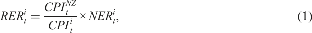
Simple averages of the monthly data were used to transform them into a quarterly frequency. The nominal exchange rate was expressed as foreign currency units per NZD. The RER for country
International visitor arrivals.
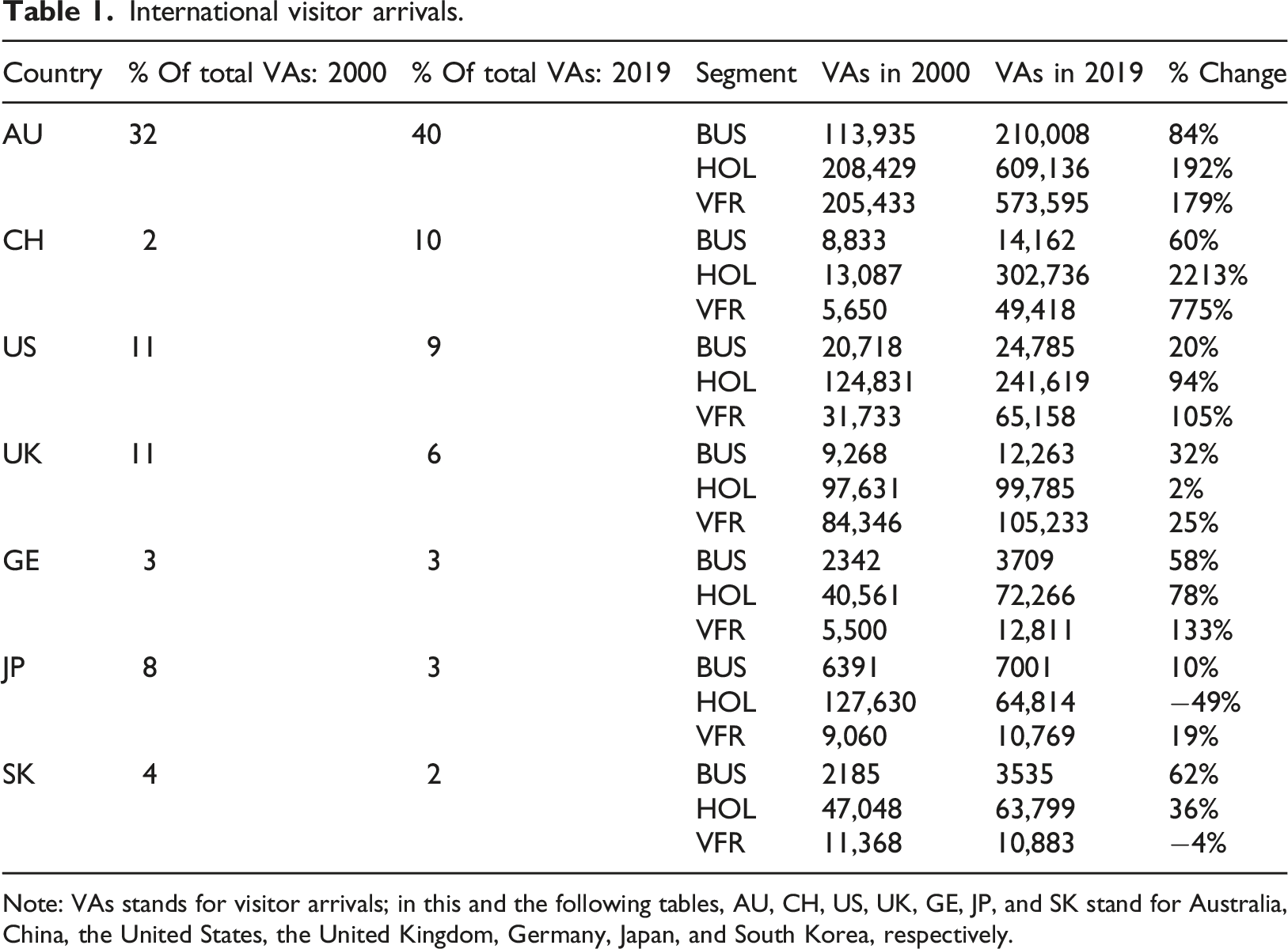
Note: VAs stands for visitor arrivals; in this and the following tables, AU, CH, US, UK, GE, JP, and SK stand for Australia, China, the United States, the United Kingdom, Germany, Japan, and South Korea, respectively.
Consider the changes in the aggregate visitor arrivals for the three segments of tourists from different countries between 2000 and 2019. Travel in each of the three segments more than doubled during this period. The number of holiday travelers from Australia, the segment registering the most substantial absolute increase, rose by 401,000 to 575,000 during this period; business travel increased by 84%, attesting to the growth of trans-Tasman trade. For China, the number of visitor arrivals in the same segment increased by 60% or 5400 travelers. Undoubtedly, Sino-New Zealand trade has increased during the last decade. However, the volume of business travel from China to New Zealand has risen only marginally in absolute terms. This segment is relatively small and has impacted overall tourism volume only incrementally. However, this may be an untapped segment that presents significant upsides. On the other hand, holiday travel from China increased more than twentyfold—in 2019, 303,000 holiday travelers arrived in New Zealand from China as compared to only 13,000 in 2000; those visiting friends and relatives increased eightfold, from 5700 to 49,000. Due to the surge in holiday travel, China constituted 10% of international tourism demand for New Zealand in 2019, up from 2% at the turn of the century.
Travelers visiting their friends and family in New Zealand accounted for the largest proportion of visitor arrivals from the United Kingdom. This is to be expected, considering the cultural ties between the two countries. Holiday travel from Japan declined by 50% between 2000 and 2019, and 4% fewer travelers from South Korea visited their friends and family in 2019 relative to 2000. Overall, New Zealand tourism has flourished during the 21st century. Even though the general trends point in the right direction, signs of plateauing in the number of visitor arrivals to New Zealand emerged in 2016. If incomes and prices were indeed the primary determinants of tourism demand, then the latter’s leveling off was likely driven, at least partly, by rising prices in New Zealand, falling incomes in tourism-importing countries, or both.
Methodological framework and empirical evidence
Stationarity properties.

Note: The statistics are associated with the Phillips−Perron tests; the equations comprise both an intercept and a trend; the null hypotheses are that the series are non-stationary; the lag length was determined using the Schwert (1989) formula:
ARDL regressions are well-suited to this analysis for several reasons: they allow for the inclusion of lagged values of the dependent as well as the independent variables in standard least square regressions—the lagged values of the dependent variable may explain changes in the destination’s popularity and trendiness, word-of-mouth, and habit formation (Song et al., 2010); each variable can be assigned a different number of lags; the long-run relationships and error correction mechanisms can be examined concurrently; as indicated above,
We specified the following ARDL model: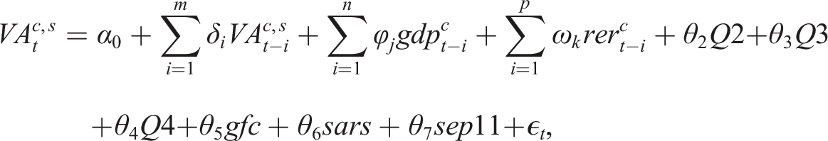
Comprising the first difference of the dependent variable, equation (3) is the conditional error correction (CEC) representation of equation (2):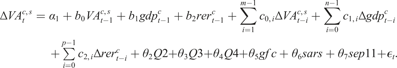
Conditional upon a maximum of four lags for the dependent variables and the regressors, the Akaike information criterion (AIC) was employed to determine the appropriate number of lags for the models. The long-run income and price elasticities were estimated from the CEC representation—these are
F Statistics from the ARDL bounds test.
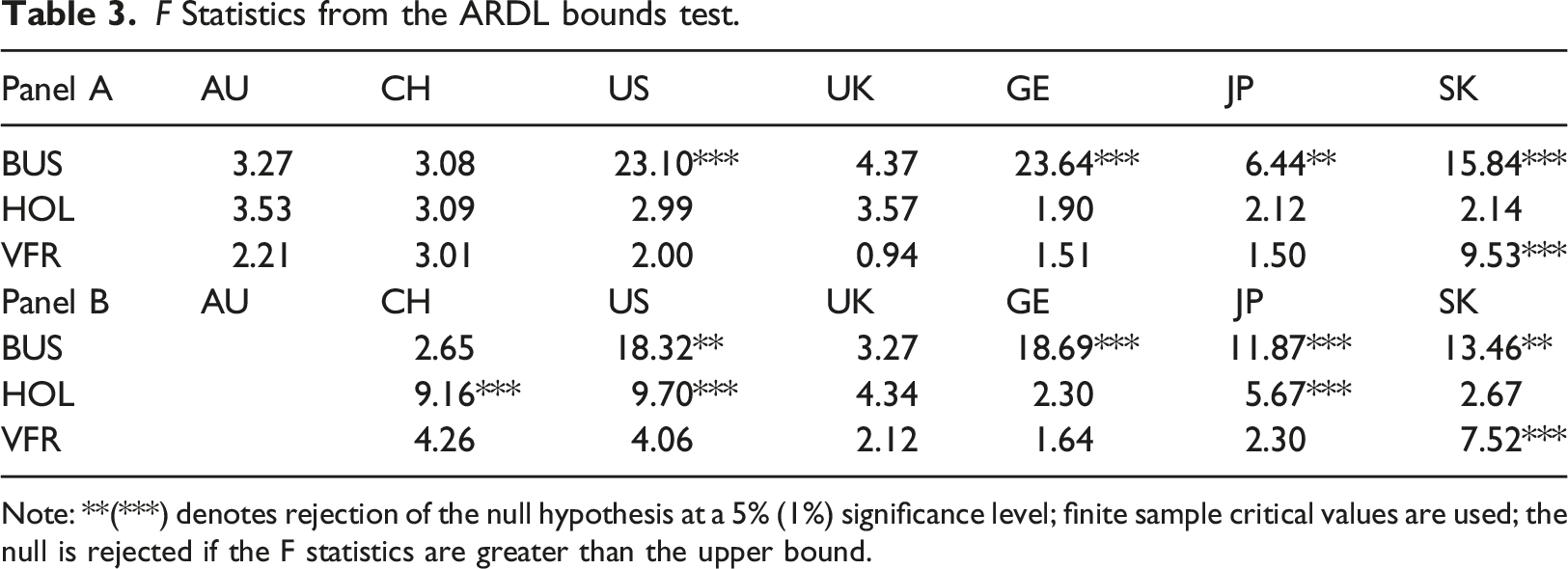
Note: **(***) denotes rejection of the null hypothesis at a 5% (1%) significance level; finite sample critical values are used; the null is rejected if the F statistics are greater than the upper bound.
ARDL models with only the real exchange rate vis-à-vis New Zealand.
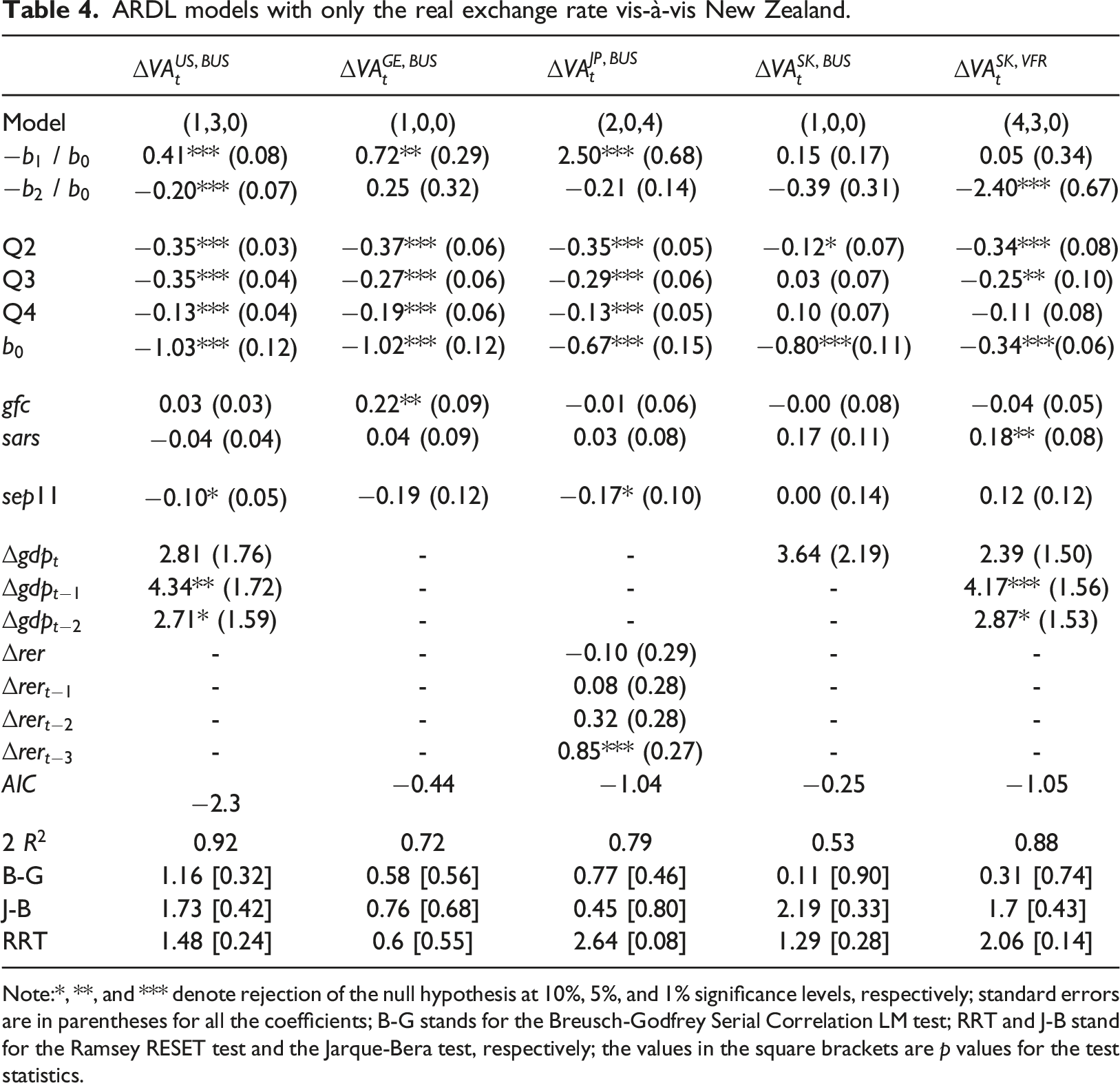
Note:*, **, and *** denote rejection of the null hypothesis at 10%, 5%, and 1% significance levels, respectively; standard errors are in parentheses for all the coefficients; B-G stands for the Breusch-Godfrey Serial Correlation LM test; RRT and J-B stand for the Ramsey RESET test and the Jarque-Bera test, respectively; the values in the square brackets are p values for the test statistics.
The long-run income-elasticity coefficients for business travelers from the United States, Germany, and Japan were 0.41, 0.72, and 2.50, respectively. Japanese business travelers were particularly responsive to changes in income, with business travel increasing by 2.5% for an increase of 1% in the GDP per capita. In contrast, business travelers from South Korea were insensitive to changes in income—the long-run income elasticity for this segment is statistically insignificant. We found a similar result for South Koreans visiting friends and relatives in New Zealand—their income elasticity was statistically zero, suggesting that their travels to New Zealand were not associated with changes in income.
We found two segments, that is, business travelers from the United States and South Korean travelers visiting friends and relatives, that were price-sensitive in the long run: the price-elasticity coefficient for the first was -0.20, and for the second was -2.40. These results suggest that higher prices were associated with lower demand for New Zealand tourism from these two segments. It bears emphasis that these segments account for a minuscule proportion of international travelers visiting New Zealand. Thus, reduced demand for tourism from this segment due to higher prices will not depress the overall demand for New Zealand tourism noticeably. The price elasticities of demand for business travelers from Germany, Japan, and South Korea were statistically zero.
The seasonal dummy variables are significant in each of the five models. This illustrates the importance of seasonality to tourism demand. Furthermore, the coefficients are negative, indicating that international visitor arrivals for most segments peaked in the first quarter. This result is interesting, as one might expect business travel to be unaffected by seasonal variations.
The estimates of
As for the short run, we found compelling evidence for a positive association between tourism demand and income for business travelers from the United States and for South Korean travelers visiting friends and relatives—the coefficients of
The importance of seasonality, however, is unmistakable—dummy variables accounting for seasonal patterns are, for the most part, significant. Notwithstanding the significance of seasonality to tourism demand in the past, whether it continues to affect tourism demand similarly moving forward remains to be seen. That the effects of seasonality will not change cannot be taken for granted.
Seasonality in tourism demand is primarily driven by weather and school and office holidays in different countries. Kulendran and Dwyer (2012) found that temperature, humidity, and hours of sunshine shape the seasonal variation in the number of tourists visiting Australia, also a long-haul destination. The recent weather events in New Zealand and the risk that climate change poses to the island nation may affect how international tourists view New Zealand as a candidate destination.
The coefficients of
We also performed various diagnostic tests. These are reported toward the bottom of Table 4. The Jarque-Bera statistics suggest that the residuals from the five models are normally distributed; the Breusch-Godfrey Lagrange multiplier tests point to the absence of serial correlation among the residuals, and the Ramsey RESET tests lend credence to the specification of the econometric models. Furthermore, the
Estimating elasticities by including the real exchange rates vis-à-vis Australia
The ARDL models above do not account for the RERs vis-à-vis Australia. We recognize the importance of investigating the elasticity of demand for New Zealand tourism by including exchange-rate-adjusted prices in Australia, a destination that, in all likelihood, features (as an alternate or complementary destination) in the plans of those visiting New Zealand. Therefore, we re-estimated income and price elasticities by including the RERs of the remaining six countries vis-à-vis both Australia and New Zealand. Although including real exchange rates vis-à-vis New Zealand and Australia in the same regression may provide insights into cross-price elasticities of tourism demand, it may also generate large standard errors and spurious estimates, rendering the results meaningless.
Accordingly, Equation (2) was augmented by adding the RERs vis-à-vis Australia as follows: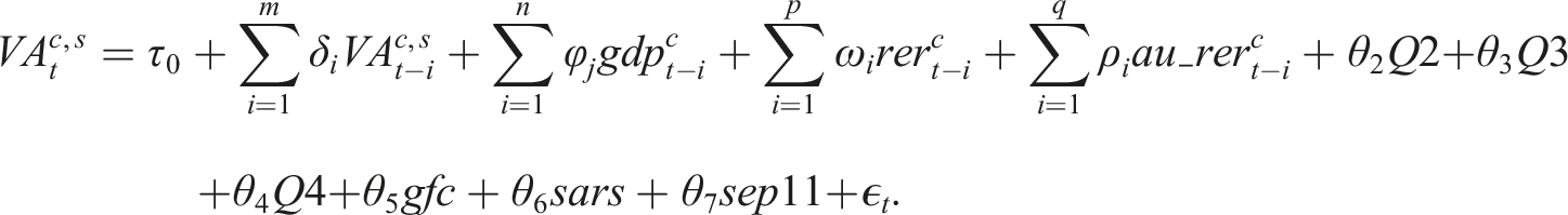
Equation (5) is the CEC representation of equation (4):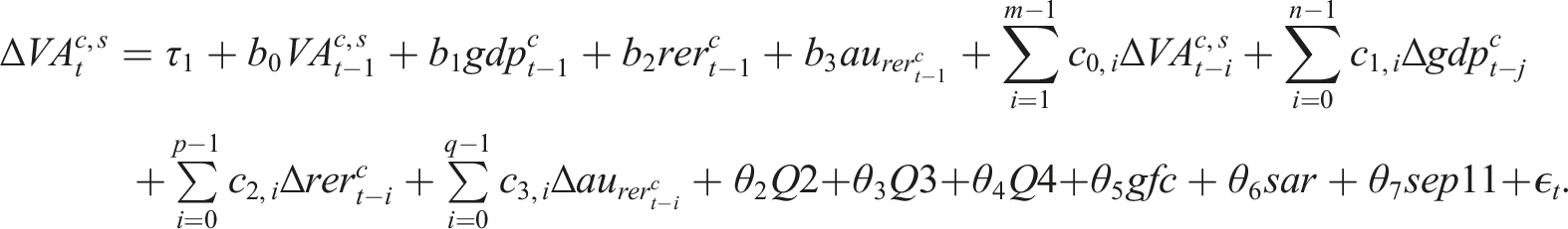
ARDL models with the real exchange rates vis-à-vis New Zealand and Australia.
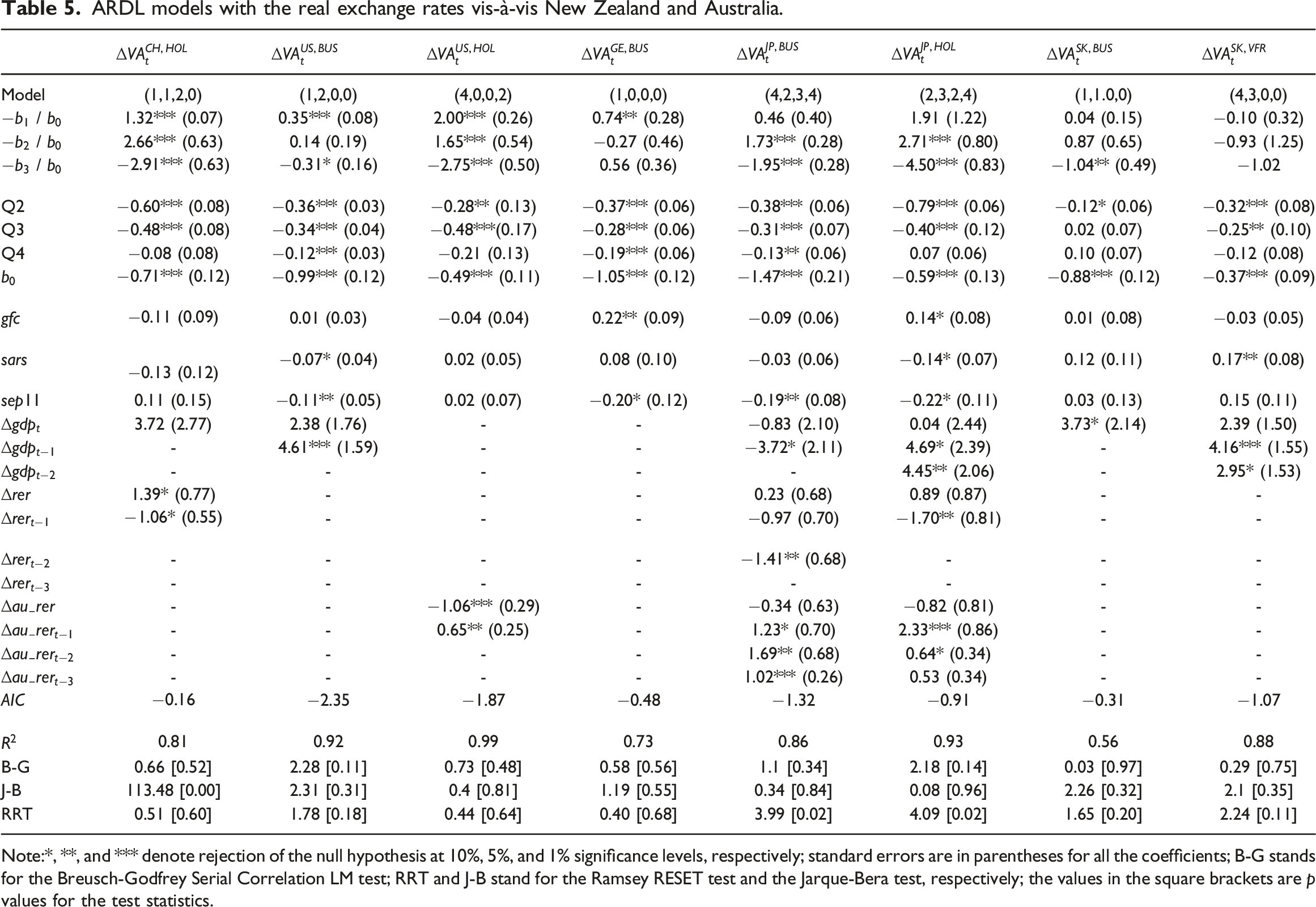
Note:*, **, and *** denote rejection of the null hypothesis at 10%, 5%, and 1% significance levels, respectively; standard errors are in parentheses for all the coefficients; B-G stands for the Breusch-Godfrey Serial Correlation LM test; RRT and J-B stand for the Ramsey RESET test and the Jarque-Bera test, respectively; the values in the square brackets are p values for the test statistics.
Unlike income elasticity, price elasticities changed considerably for each segment. Two points stood out apropos the results for the long run: first, tourism demand was positively associated with the RERs vis-à-vis New Zealand for four segments; second, it was negatively associated with the RERs vis-à-vis Australia for six segments. The models comprising the real exchange rate vis-à-vis Australia yield positive price elasticities, indicating that rising prices were associated with higher demand for New Zealand tourism.
The positive price elasticities are likely artifacts of the model specification. As expected, using both real exchange rates may lead to multicollinearity and produce spurious elasticity estimates, calling the veracity of these models and the results they produce into question. Our results suggest that tourism demand models should avoid using real exchange rate series vis-à-vis multiple countries simultaneously.
The coefficients of the seasonal dummy variables and the variables representing the global financial crisis, the SARS outbreak, and the September 11, 2001 terrorist attacks are similar across the two sets of models. Like the results reported in Table 4, income elasticities are larger in the short run than in the long run. In the case of South Korean travelers visiting friends and relatives, the short-run income elasticities produced by the two models are strikingly similar.
Concluding remarks
We estimate the income and price elasticities of international demand for New Zealand tourism. Short- and long-run elasticities are provided for three segments—holiday travelers, business travelers, and those visiting friends and relatives—from the seven most significant tourism-importing countries. The inherent differences in the profiles, motivations, and proclivities of different segments of travelers motivated us to consider a disaggregated approach (Song and Li, 2008; Peng et al., 2014). This approach provides granular insights that industry stakeholders and policymakers can use to formulate targeted initiatives and policies. In the long run, there is limited evidence pointing to the international demand for New Zealand tourism being income-sensitive; the evidence for price sensitivity is still weaker. Seasonal effects significantly affect tourism demand; somewhat surprisingly, the volume of business travel also exhibits seasonal patterns.
Arbitrage in foreign exchange markets ensures instantaneous adjustments of different bilateral exchange rates, causing many currencies to co-move. In light of this comovement, using multiple variables constructed with the same underlying constituents may yield misleading results. Two common examples in tourism research are RERs vis-à-vis different countries and RERs comprising the same CPIs. However, collecting more data of the same kind is unlikely to resolve this issue. Instead, primary data from surveys and interviews may help untwine the effects of prices on international demand for tourism. While this is a promising line of research, we recognize that such data can be difficult and costly to obtain. Therefore, we propose that the results obtained from different model specifications are duly compared, contrasted, and reported. This would provide a more balanced perspective to stakeholders. Considering the inexactitude inherent in quantitative assessments of social phenomena, approaches that triangulate results from different methods and model specifications are in order.
With advancements in web analytics and big data tools and techniques, collecting and transforming data into actionable insights is technically feasible, and the costs of doing so are progressively falling. As a result, opportunities for analyzing more granular data abound. Such analyses would help identify different archetypes of tourists and provide insights into their preferences and behaviors. These insights may inform the design and implementation of hyper-targeted marketing initiatives and personalized tourism packages. Accordingly, we propose three avenues for future research: first, in partnership with industry stakeholders, collect primary data on tourists’ profiles and willingness to pay in order to identify causal impacts of hypothesized determinants of tourism demand; second, collect and analyze web data to draw insights into tourists’ sentiments and perceptions regarding specific tourist destinations—these insights can point the researcher to meaningful quantitative analyses; third, confirm the results of this study in the context of other long-haul destinations worldwide.
These findings have significant implications for policymakers and industry stakeholders. In the short run, tourism demand is relatively resilient to price shocks. However, adverse income shocks may reduce the demand for New Zealand tourism among certain segments. In response to this, stakeholders in the tourism industry can develop suitable initiatives and diversified offerings to address the drop in demand caused by economic recessions in specific markets. For instance, if there is an economic downturn in the United States, resulting in a decline in business travelers arriving in New Zealand, targeted marketing initiatives could be devised to attract domestic tourists and visitors from other international markets.
Footnotes
Declaration of conflicting interests
The author(s) declared no potential conflicts of interest with respect to the research, authorship, and/or publication of this article.
Funding
The author(s) received no financial support for the research, authorship, and/or publication of this article.