Sage Journals: Discover world-class research

Abstract

Does two-party competition in the United States lead to improved human welfare spending? The debate over the merits of competition has gained traction yet again in the study of American politics. Gerald Gamm and Thad Kousser suggest that from 1880 to 1980 two-party competition led to desirable outcomes like increased education, transportation, and health spending. The modern panel data presented here suggest the spending effects do not persist beyond 1980 through 2020, and also, there is a negative effect on economic growth stemming from state-level partisan competition. The reversal of the historical trend is justified by predictions from existing formal models: at particularly high levels of baseline political competition, the effect of additional competition on growth is ambiguous.

Keywords

historical political economy state politics party competition

Introduction

Does two-party competition in the United States lead to improved human welfare spending and economic growth? Why or why not? And has the effect of two-party competition changed over time? In this brief research note, I present a concise literature review, an extension of the difference-in-differences model used by Gamm and Kousser (2021), and a justification for the findings using the formal model from Besley et al. (2010).

Literature review

Gamm and Kousser

Gamm and Kousser divide their recent APSR piece into two sections. First, they find that between 1880 and 1980, political competition had significant positive effects on spending in three areas: transportation, education, and healthcare. Second, they show that the increased spending by state governments on transportation, education, and healthcare induced a lagged effect on quality of life outcomes: decreased infant mortality, higher average education levels, longer life expectancy, and higher incomes. In this work, I do not probe the second part of their design. It is accepted that spending improves quality of life.

Gamm and Kousser study their first question by estimating difference-in-differences models with the left hand side as some state-level spending outcome (education, transportation, or health) and the right hand side as state and year fixed effects, state-level controls, and the main variable of interest: competition.

τ_{s t} = θ_{s} + ν_{t} + γ X_{s t} + δ k_{s t} + ϵ_{s t}

Gamm and Kousser report statistically and substantively significant effects (δ) on state-year competition ( k _st). In their study, competition comes from the state legislature. The way they measure the level of competition in a state-year is to subtract the average margin of control in the two chambers of the state legislature from 100. So at the extremes, for example, if Democrats hold all of the seats in both chambers of the state legislature then the margin of control is 100 and the competition metric is 0. If the seats are split evenly then the margin of control is 0 and the competition metric is 100.

The theory sustaining their work is that parties give members the incentives to pursue the collective good and foster the strong coalitions necessary to pass legislation (Aldrich and Griffin 2018). According to this view, competition amplifies the effects of constructive electoral incentives and strong policy coalitions. They refer to the first mechanism as “motivation,” contending that in competitive environments legislators will forgo individual rewards and pursue statewide programs. The second mechanism they call “means,” arguing that when one party dominates, factions emerge within the dominant party and infighting weakens the power to carry out sustained action (Key 1949).

Gamm and Kousser’s findings diverge from a pattern of null effects in the two-party competition literature. Rogers and Rogers (2000) study competitive gubernatorial races with the outcome of interest as government size. The study measures government size with both revenue and expenditure and the authors find no positive link between government size and political competition. They use state and year fixed effects and panel data from 1950 to 1990. Besley and Case (2003) find frequent null results in both political science and economics in an extensive literature review. In addition to null effects on competition, a range of papers across time and discipline have found null effects on the party in power as it affects growth and spending (Dynes and Holbein 2020; Winters 1976).

By design, Kousser and Gamm’s period of study on two-party competition and spending ends in 1980. An impetus for my paper was to see what happens when applying a similar design to 1980 through 2020. We may expect the effect of competition on growth and spending to change after 1980. As Kousser and Gamm write in their conclusion, “American politics began changing profoundly in the 1980s. These last four decades have been a time of unremitting and closely fought party competition in national politics, new social and cultural cleavages, historically high levels of partisan polarization, a collapse in mediating institutions, shifting norms and rules in Congress, geographic sorting, and the growth of social media” (Gamm and Kousser 2021).

Besley, Persson, and Sturm

Moving backwards in time to a 2010 paper in The Review of Economic Studies, Timothy Besley, Torston Persson, and Daniel M. Sturm create a full formal model, derive the equilibrium behavior of the two parties, and test the theoretical claims with an empirical case study using the U.S. states 1950–2001. In this section, I review their main empirical contribution and in the next I explore the theoretical political model.

The regressions they run are of the same baseline form as that mentioned above.

τ_{s t} = θ_{s} + ν_{t} + γ X_{s t} + δ k_{st} + ϵ_{s t}

Now, however, τ_st is a “policy stance” that parties strategically choose as they calculate electability and rents once in office. They use three concrete economic outcomes to proxy for the theoretical τ: total state tax revenue as a percentage of personal income, infrastructure spending, and whether a state has a right-to-work law (Besley et al., 2010).

Also, competition k _st is measured differently. Instead of using margins in the state legislature, the authors look at the average Democratic voteshare across directly elected state offices¹ and subtract it from 0.5. Formally, k _st = −|d_st − 0.5| where d_st is the Democratic voteshare in state s and time t. For example, at extremes of Democratic voteshare, d_st = {0%, 100%}, the competition metric is minimized at −0.5, and at an even vote split, d_st = 50%, k _st is maximized at 0.

Using specifications without and with state-year controls, there are statistically and substantively significant results on all three outcomes. Competition is associated with pro-business policy outcomes. The finding holds under robustness checks: adding in a diverse set of state-year controls, allowing the South to vary in a non-parametric way through indicator variables and interaction terms, and instrumenting for competition through the government intervention of the VRA. Precisely, the IV approach instruments competition with the share of the population subject to a literacy or poll tax pre-1965 VRA, and 0 post-1965. The authors include the IV robustness check to address endogeneity concerns, or the (likely) possibility that there is reverse causation of policy choices on competition.

The underlying mechanism is that swing voters, whose voting decision is based on parties’ economic policy choices, only start to gain electoral influence if political competition falls within a threshold. That is, within a range of competition k_L → k_H, the parties push each other to make growth-promoting policy choices to win undecided voters. The pro-spending empirical results are thought to come from a mid-range competition environment. The authors bucket the continuous competition variable k_st into discrete categories and find that middle levels boast the strongest positive effects. An advantage of the theory from Besley et al. (2010) is that it comes from a model that deals with the interaction between voters and politicians. Recent work in political economy has emphasized the importance of bridging the gap between voter-based and officeholder-based explanations of political phenomena (Ashworth and Fowler 2020).

Critically, their model has non-linear predictions for the effect on competition. The next section explains them.

Theory

There are three reasons to predict a different relationship between competition and spending from 1980 through 2020 as compared to 1880 through 1980.

High baseline competition

Today, there are roughly equal numbers of devoted partisans in the two major parties especially when subsetting to likely voters from the full eligible public (Kennedy and Keeter 2019). As a result, there are consistently competitive national races. Political science work has documented the dominance of the Democratic party in the twentieth century. There was room for competition to promote growth and voter welfare. But now, with such high baseline competition, more competition may in fact suppress what voters want. Parties can shirk while maintaining their competitiveness in national and state races.

The main equilibrium proposition from Besley et al. (2010) offers structure to this hypothesis. A competition measure k is calculated from the share of partisans in the population, the advantaged party’s lead in the share of devoted partisan voters, and the salience of economic issues to non-partisan voters.2

The equilibrium proposition is:

(i) For k below a lower threshold k_L, the advantaged party pursues their own preferred (anti-growth) policy and wins for sure.

(ii) For k in an intermediate range k_L → k_H, the disadvantaged party picks more pro-growth policies than the advantaged party. As competition increases, the probability that the disadvantaged party wins increases and the advantaged party moves toward pro-growth policies.

(iii) For k close enough to zero, the party ranking and the effect of political competition on policy and economic growth are ambiguous.

Stated once more: At low competition below k_L, the dominant party can forgo growth and still win despite increasing competitiveness. The dominant party will win while pursuing an anti-growth platform. At exceptionally high levels of competition above k_H, when the lagging party improves its chances of winning thereby making the race tighter, the lagging party can simultaneously pursue and implement elite rent-seeking over public facing growth while maintaining the coin-flip nature of the election. For this reason, increasing competition from an already high baseline level between 1980 and 2020 may have taken away from voters instead of providing for them.

Polarization

On average, representatives now are more extreme than they were in the twentieth century. More extreme candidates have incentives to run for office even though voters prefer moderates (Hall 2019). The logic behind Gamm and Kousser (2021) was that party competition promotes spending because it leads to strong intra-party bonds; members create strong policymaking coalitions that last over time and legislators feel bound to their wider state constituencies instead of self-interest. However, strong ideological and affective polarization paired with higher competition in the electorate creates the incentive for representatives to make the opposition look worse at whatever cost, even forgoing their constituents’ well-being to do so. Furthermore, there is the simple polarization-based explanation for a reversed effect on competition which is that extreme candidates will find it more difficult to compromise with out-partisans on budgets.

Nationalization of state politics

Recent work in political science has documented the nationalization of politics (Hopkins 2018). That is, state races are increasingly determined by what is happening on the national scale. If voters are looking to national political conditions even when they vote for their state legislatures, then we should see minimal effects on seat share competition in the state legislature and instead a strong effect on national electoral competition. This explanation would say, it is not that the effect of state based political competition has changed, but rather that is has been upstaged by national competition.

Main contribution

I update the findings from Gamm and Kousser (2021) to see if they hold on modern panel data from the states. The empirical strategy is similar to the one introduced in the papers above. I add the outcome of state GDP per capita to the list of health, education, and transportation spending. I find the effects of party competition have changed over time. While party competition drove growth and spending from 1880 up to 1980, there was a shift, and between 1980 and 2020, party competition has null or negative effects.

Empirical approach

I run difference-in-differences models with state and year fixed effects. The idea being that state fixed effects θ_s hold constant differences between states and year fixed effects ν_t absorb common shocks across all states in specific years. I cluster standard errors by state. The models take the form

τ_{s t + 1} = θ_{s} + ν_{t} + γ X_{s t} + δ k_{st} + ϵ_{s t}

The spending and growth outcomes (τ) and the competition metrics ( k _st) are explained below. X_st is a matrix of relevant covariates based explicitly on the design of Gamm and Kousser (2021): income; partisanship of the governor, state senate, and state house; and census data on race, urbanization, and immigration (Ruggles et al., 2021).

Outcomes and data

The outcomes are represented as τ_st+1 because it is assumed that a given state legislature impacts the spending patterns and economic growth for the following year. The outcomes studied here are per capita elementary and secondary education spending, transportation spending, health spending, and state-level GDP per capita. Annual data on state-level education and transportation spending comes from the National Association of State Budget Officers³ (Nass 2021), data on health spending comes from the Centers for Medicaid and Medicare services (Lassman et al., 2017), and data on state-level GDP comes from the Bureau of Economic Analysis (Siebeneck 2021).⁴ All dollar amounts are converted to per capita 2016 constant dollars for internal consistency and comparisons with Gamm and Kousser (2021) who also use 2016 constant dollars. See Figure 1 for time series growth plots of upwards trending outcomes.

Figure 1.

Average outcomes (per capita 2016 dollars).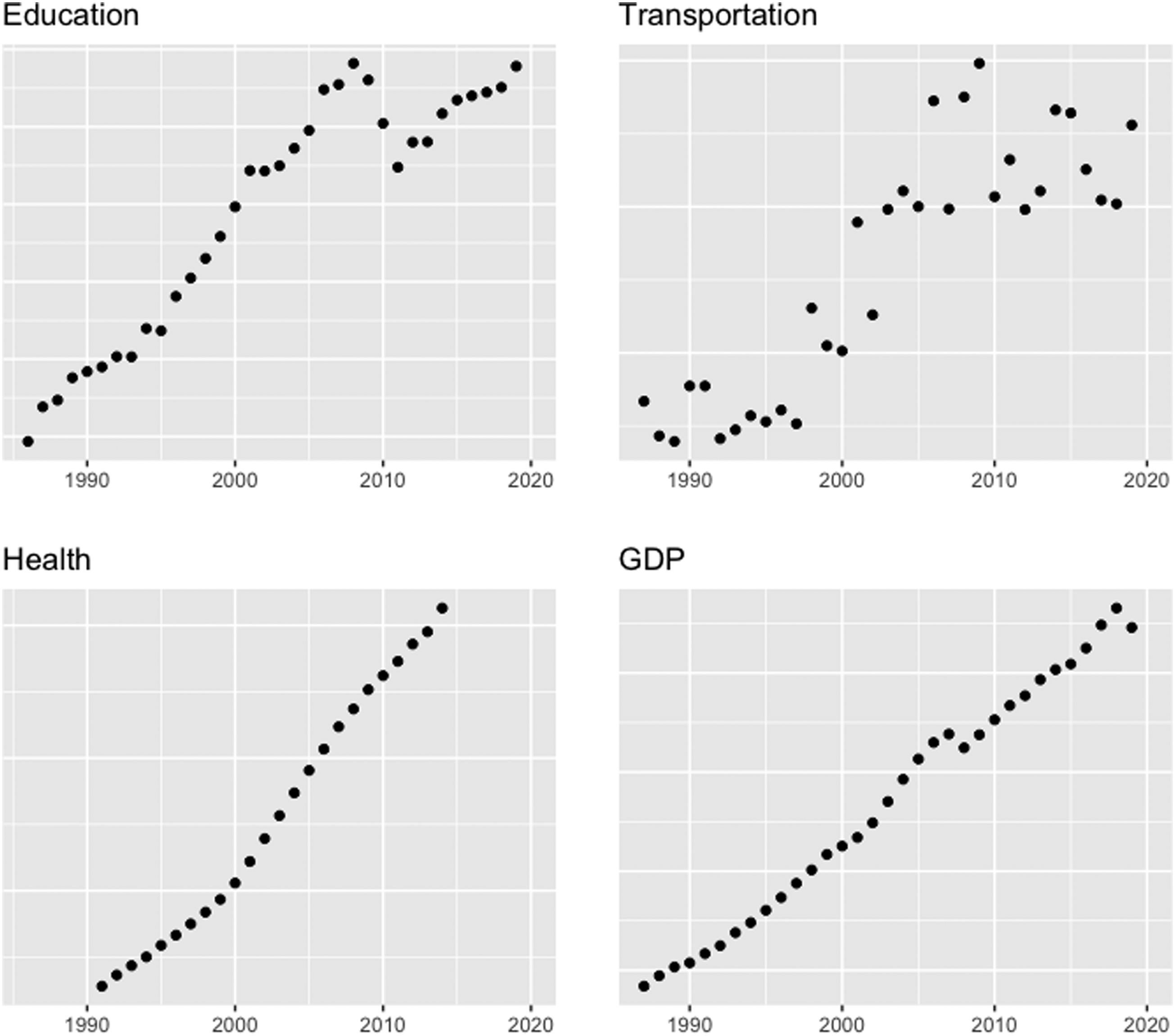

Party competition data

There are many different ways to measure party competition, with the Ramney Index being the most common (Holbrook and Van Dunk 1993). The Ramney Index is measured by averaging the seats won by Democrats in the upper and lower state chambers along with the Democratic gubernatorial voteshare. The measure Gamm and Kousser (2021) and I use is slightly more limited, it is an average of seat control in the upper and lower state legislature chambers. I will refer to this as “legislative party competition.” The legislative seat share data comes from Klarner (2013) through 2011 and then pivots to the National Council of State Legislatures (Williams 2022) through 2020. I leverage the data availability of the modern period of analysis to take measurements of competition every election year. I have over 1,500 state-year observations in my 40 year period of analysis as compared to fewer than 400 state-year observations across 100 years in Gamm and Kousser (2021).

As mentioned above, Besley et al. (2010) use a separate metric developed by Ansolabehere and Snyder (2002) that looks at election results for state offices ranging from congressional representatives to down-ballot races like secretary of state. Competition is calculated as − |d_st − 0.5| where d_st is the share of the vote for Democrats across elections. Higher (less negative) values correspond to more party competition. I will refer to this as “electoral competition.⁵” I calculate electoral competition for each state-year by looking at the most recent national election cycle’s average voteshare for congresspeople and the president.⁶

Electoral competition does in fact measure something different than legislative party competition. The correlation coefficient between these two variables in my data is .475, and the correlation coefficient for Gamm and Kousser (2021) is .629. Electoral competition has often been considered a control variable, part of X_st in the formal statement. However, a priori it is just as valid an indicator for the true latent political competition in a state. Therefore, I consider it a part of the vector of interest δ k _st in the formal statement. In my discussion of results, I consider effects on both “legislative party competition”—the seat share calculation, as well as “electoral competition”—the voteshare calculation.

Results

The main takeaway from the results in Table 1 is that the coefficients on legislative party competition are negative, and of about the same magnitude as those reported by Gamm and Kousser (2021).

Table 1.

Main results.

	Outcome (per capita):
	Education		Health		Transportation		GDP
	(1)	(2)	(3)	(4)	(5)	(6)	(7)	(8)
Legislative competition	− 0.919	− 0.502	− 4.759	− 5.007	− 0.530	− 0.447	− 42.463	− 27.737
Legislative competition	(1.248)	(1.014)	(2.421)	(1.692)	(0.622)	(0.542)	(20.649)	(15.370)
Electoral competition		− 0.247		− 0.186		0.648		− 1.776
Electoral competition		(0.730)		(1.785)		(0.464)		(13.388)
Income		0.006		0.010		0.003		0.210
Income		(0.003)		(0.009)		(0.003)		(0.056)
D Governor		16.651		32.035		22.957		920.403
D Governor		(28.625)		(49.243)		(17.737)		(331.345)
D Senate		91.925		99.465		− 2.579		397.031
D Senate		(39.137)		(54.803)		(13.145)		(338.632)
D House		74.163		146.609		1.529		661.610
D House		(37.993)		(62.906)		(18.179)		(301.280)
Foreign-born %		− 11.063		− 231.311		− 5.411		− 229.202
Foreign-born %		(17.786)		(56.602)		(10.703)		(309.398)
Black %		43.079		151.190		− 4.774		892.719
Black %		(21.166)		(64.400)		(12.483)		(330.407)
Other nonwhite %		− 6.956		78.907		1.273		627.929
Other nonwhite %		(12.946)		(52.318)		(10.921)		(215.961)
Urban %		− 1.658		− 12.426		− 1.105		− 54.454
Urban %		(2.802)		(7.249)		(1.338)		(84.664)
Outcome mean (1986–2020)	$1089.81		$5142.81		$521.58		$36,270.67
Observations	1686	1534	1200	1156	1686	1534	1700	1548
R²	0.792	0.814	0.971	0.980	0.811	0.841	0.944	0.964
Two-way F.E.	Y	Y	Y	Y	Y	Y	Y	Y

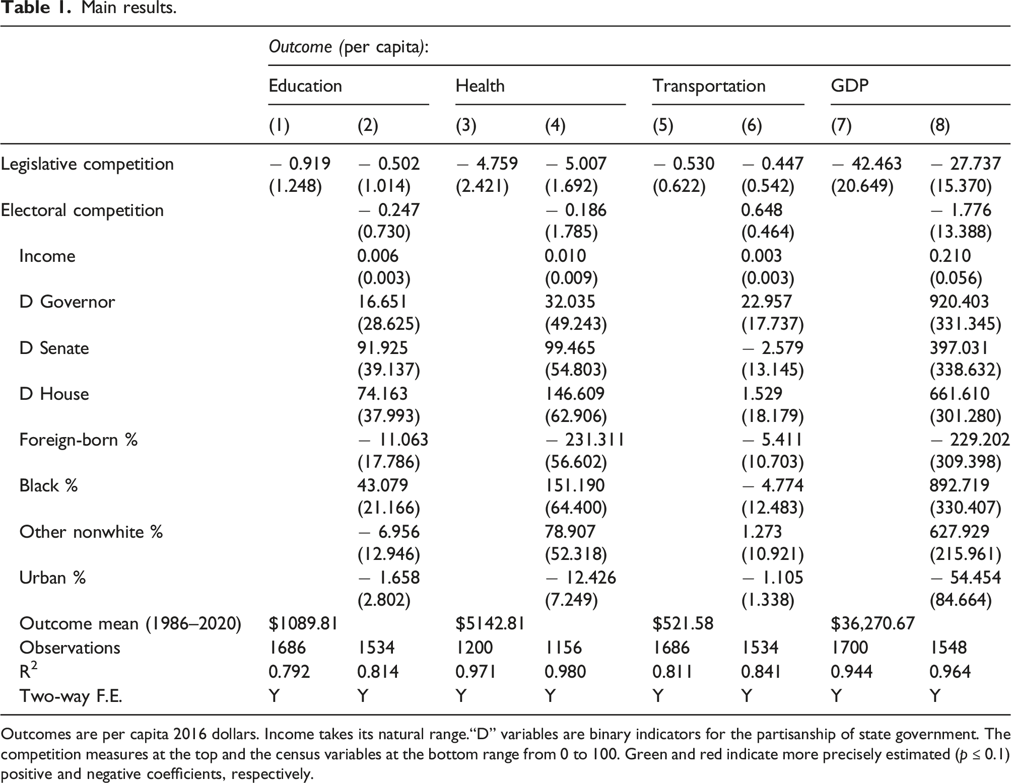
Outcomes are per capita 2016 dollars. Income takes its natural range.“D” variables are binary indicators for the partisanship of state government. The competition measures at the top and the census variables at the bottom range from 0 to 100. Green and red indicate more precisely estimated (p ≤ 0.1) positive and negative coefficients, respectively.

GDP and health spending

The effects of legislative party competition on GDP and health are large, negative, and significant. Coefficients in these models are estimated with the same negative sign for both competition metrics, with the statewide legislative competition metric estimated precisely. Consider a state that switches from no party competition to full party competition. In other words, consider a state that switches from the Democrats holding every seat in both chambers of the state legislature to a 50–50 split. By the more conservative models using controls, that is, a 9% hit to GDP and health spending. If that seems extreme, we can do a similar calculation with the mean range of legislative party competition across the sample (41.1/100). When a state moves from low to high across the average range of competition, that state sees a 4% point dip in GDP and health spending. Texas, for instance, fits this profile. Texas moved from a legislative competition score of about 63.6 in 1990 to a score of 99.8 just 10 years later in 2000.

Education and transportation spending

None of the coefficients on the competition metrics in the education and transportation models are estimated to be statistically different from zero. The coefficients on legislative competition are negative and the electoral competition coefficients are positive. But both have relatively large state-clustered standard errors. Even the coefficients on indicators for the partisanship of state government are imprecisely estimated in the transportation model. This is further evidence of null effects on the party in power (Dynes and Holbein 2020).

While education and transportation do not show statistical significance here, I can confirm they are statistically different from those values reported in Gamm and Kousser (2021) by combining data and running the regression on the full set 1880 to 2020.⁷ I create an indicator variable for the modern period 1980–2020 and look at the coefficient on the interacted term. If the effect on competition has not changed at all between our two studies, then we should see coefficients close to 0 on the interacted terms. If it is still the case that competition brings about increased spending, the coefficients on the competition metrics should be uniformly positive and similar to those in the original study.

However, that is not what we see. In Table 2, beginning with legislative competition, the picture emerging from both models is that competition used to be associated with increased spending, but in the modern period that has changed. The effect drops to a negative one. With regard to electoral competition, in the education model neither term is measured precisely. Surprisingly, in the transportation model, the negative early period effect switches to a positive effect in the modern period. Looking at Table 1 in the original Gamm and Kousser (2021) study, electoral competition has a negative coefficient across the board, with a large and significant effect in the transportation model. The portrait painted by these data is ambiguous. We see a coefficient on the seat share margin pointing in one direction, and a coefficient on the vote share competitiveness pointing opposite. The true level of two-party competition can be thought of as a latent variable, and the metrics we have are coarsened, slightly distorted versions of it. Taking both of the measures we have available into account, recent US competition does not promote social spending.

Table 2.

Interacted models.

	Outcome (per capita):
	Education	Transportation
	(1)	(2)
Legislative competition	1.800**	0.744
	(0.768)	(0.463)
Legislative competition * modern	− 2.139*	− 1.511**
	(1.150)	(0.690)
Electoral competition	0.287	− 1.706**
	(0.991)	(0.753)
Electoral competition * modern	− 0.947	1.921**
	(1.507)	(0.834)
Observations	1914	1891
R²	0.856	0.845
State and year F.E.	Y	Y
Census and party controls	Y	Y

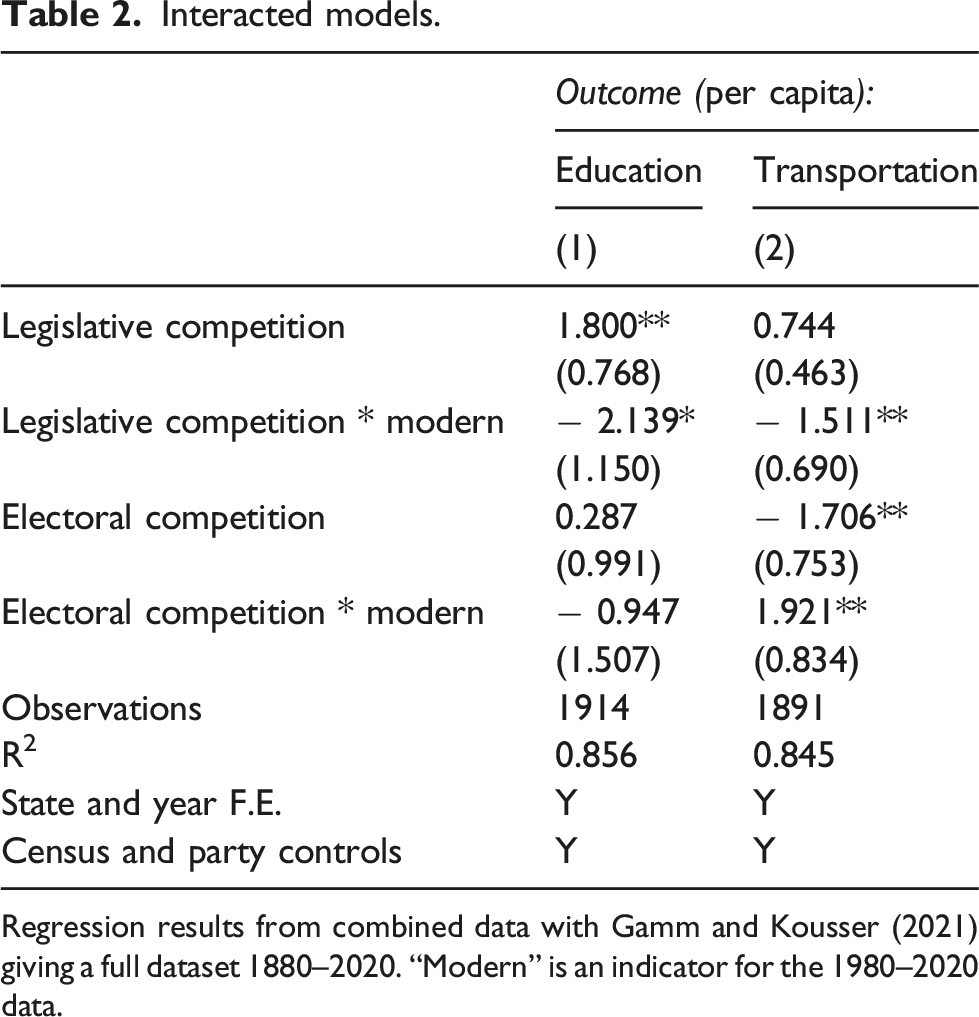
Regression results from combined data with Gamm and Kousser (2021) giving a full dataset 1880–2020. “Modern” is an indicator for the 1980–2020 data.

GDP and education, transportation, and health spending all capture something unique about a state’s priorities and economic well-being. Taken together, the effects on competition in this brief research note are mostly null, and point negative when they are strong.

Conclusion and future work

The data support the theory that we are at a high baseline level of competition, past the ceiling on the threshold in which more competition is growth-promoting. Figure 2 shows electoral and state legislative competition from 1880 to 2020. Each point is an average across all states in a given year. In black is state legislative competition with one horizontal line for the 1880–1980 average and one horizontal line for the 1980–2020 average. Both competition metrics are higher now than before. In particular, the state legislative metric’s steep rise in the late twentieth century aligns with expectations of the one party South.

Figure 2.

Average competition by year (combined data).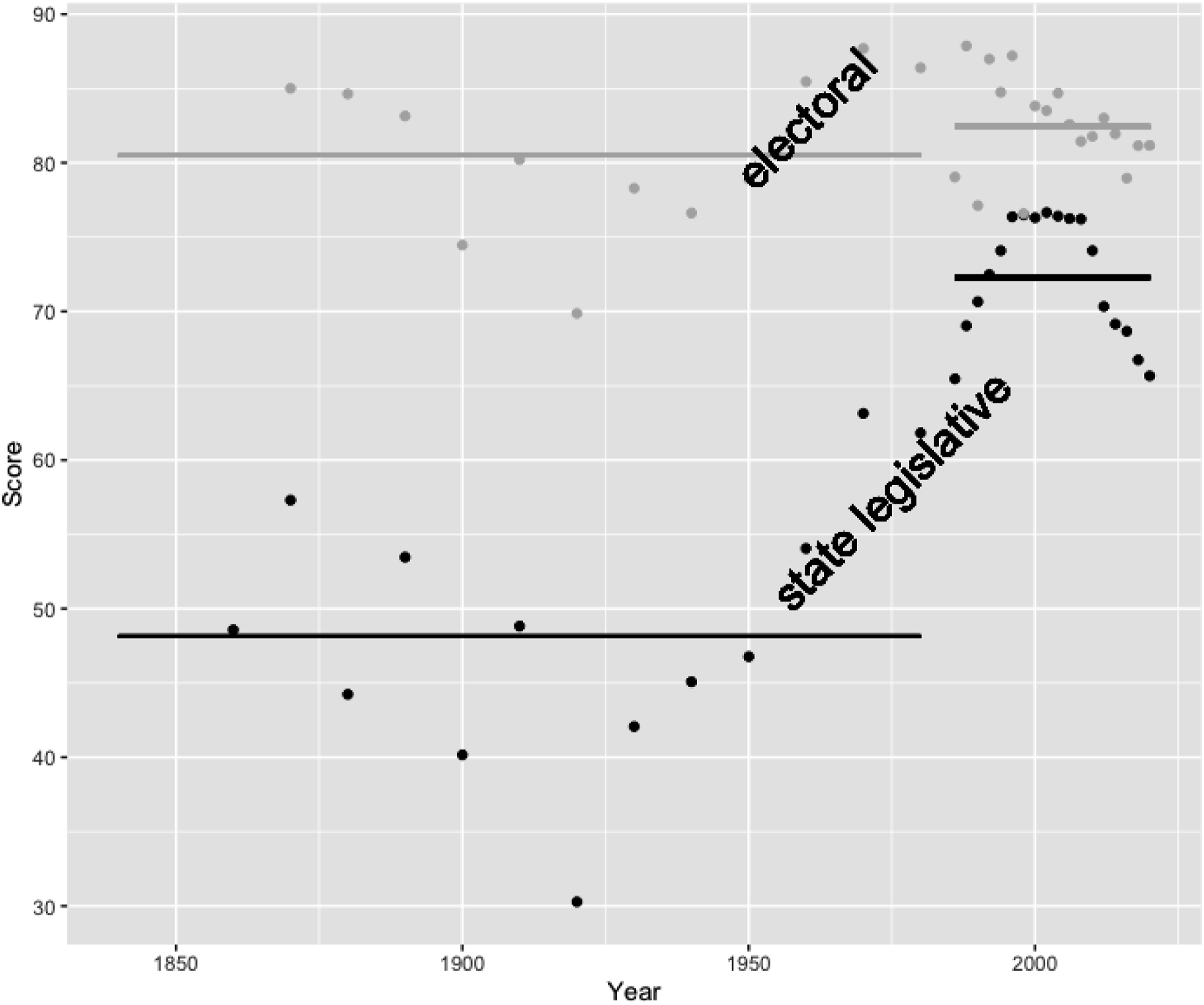

Why has two-party competition exceeded the ceiling on the threshold in which it is growth-promoting? Because more Americans are now self-identified independents and the Democratic advantage among self-identified partisans has shrunk (Pew 2015). We have polarized parties and voters sorting themselves into these parties ideologically. Party sorting, polarization, and the calcified economic positions of the two parties would suggest that the true independents who are undecided year to year are that way because of non-economic issues (Fiorina 2002).

More work is needed to explore the relationships between polarization, nationalization, and competition. However, this preliminary evidence suggests that the nationalization explanation is unlikely. We do not see an increasingly large effect on national electoral competition and a decreasing effect on state legislative competition. In the modern period, there is still a state competition effect but its sign has flipped.

Future work

This research note has extended the period of analysis from difference-in-differences models in Gamm and Kousser (2021) and justified negative and null findings by using a formal model from Besley et al. (2010). There are a few points that future work should consider.

First, the observational strategy here can be stronger. There are weaknesses in the identification strategy from the observational panel data. The weaknesses of difference-in-differences in this setting are well documented. A natural experiment would be better. Is there an intervention that creates an exogenous shock to competition that can be studied as a natural experiment? It is difficult to think of one, and that is why studies to date have focused on observational panel data. I explored non-partisan redistricting commissions for the purpose of a natural experiment. I looked into this by seeing if there was a first stage effect on party competition via the adoption of a redistricting commission. Of the six states that adopted a redistricting commission between 1980 and 2020, I found no first stage effect of redistricting commission on competition. Researchers can consider other such “shocks” and justify their as-if random implementation as an experiment.

Second, competition may not operate at the state level. There is good reason to believe that competition in cities and counties matters more for economic outcomes than state-level competition. Indeed, the state-level competition measures we have available are quite coarse. A more convincing analysis looking at two-party competition in the United States would show a pattern across thousands of counties instead of dozens of states.

Supplemental Material

Supplemental Material - Two-party competition in the United States: Reversed growth trends

Supplemental Material for Two-party competition in the United States: Reversed growth trends by Graham Straus in Party Politics

Footnotes

Declaration of conflicting interests

The author(s) declared no potential conflicts of interest with respect to the research, authorship, and/or publication of this article.

Funding

The author(s) received no financial support for the research, authorship, and/or publication of this article.

ORCID iD

Graham Straus

Supplemental Material

Supplemental material for this article is available online.

Notes

Author biography

Graham Straus, is a political science PhD student at UCLA focusing on American political behavior and methodology. He is concurrently pursuing a masters in statistics. Current projects range from studying the occupational backgrounds of city council members to analyzing survey experiments focused on persuasion in parallel and COVID vaccine uptake. He manage the UCLA national voter file. He graduated from Brown with a dual degree in political science and math.

References

Aldrich

Griffin

(2018) Why Parties Matter: Political Competition and Democracy in the American South. In: Chicago Studies in American Politics. Chicago, IL: University of Chicago Press.

Ansolabehere

Snyder

(2002) The Incumbency Advantage in U.S. Elections: An Analysis of State and Federal Officess, 1942-2000. Election Law Journal 1(3): 315–338.

Ashworth

Fowler

(2020) Electorates versus Voters. Journal of Political Institutions and Political Economy 1(3): 477–505. URL. DOI: 10.1561/113.00000016. http://www.nowpublishers.com/article/Details/PIP-0016

Besley

Case

(2003) Political Institutions and Policy Choices: Evidence from the United States. Journal of Economic Literature 41(1): 7–73. DOI: 10.1257/002205103321544693

Besley

Persson

Sturm

(2010) Political Competition, Policy and Growth: Theory and Evidence from the US. Review of Economic Studies 77(4): 1329–1352. DOI: 10.1111/j.1467-937X.2010.00606.x

Dynes

Holbein

(2020) Noisy Retrospection: The Effect of Party Control on Policy Outcomes. American Political Science Review 114(1): 237–257. Cambridge: Cambridge University Press.

Fiorina

(2002) Parties and Partisanship: A 40-Year Retrospective. Political Behavior 24(2): 93–115. Springer, URL https://www.jstor.org/stable/1558351

Gamm

Kousser

(2021) Life, Literacy, and the Pursuit of Prosperity: Party Competition and Policy Outcomes in 50 States. American Political Science Review 115: 1442–1463. DOI: 10.1017/S0003055421000617

Hall

(2019) Who Wants to Run?: How the devaluing of political office drives polarization. In: Chicago Studies in American Politics. Chicago, IL: University of Chicago Press. URL https://press.uchicago.edu/ucp/books/book/chicago/W/bo35612049.html

10.

Holbrook

Van Dunk

(1993) Electoral Competition in the American States. American Political Science Review 87(4): 955–962. DOI: 10.2307/2938827

11.

Hopkins

(2018) The Increasingly United States: How and Why American Political Behavior Nationalized. In: Chicago Studies in American Politics. Chicago, IL: University of Chicago Press. URL https://press.uchicago.edu/ucp/books/book/chicago/I/bo27596045.html

12.

Kennedy

Keeter

(2019) Why Public Opinion Polls Don’t Include the Same Number of Republicans and Democrats. Washington, DC: Pew Research Center.

13.

Key

(1949) Southern Politics in State and Nation. New York, NY: Knopf.

14.

Klarner

(2013) State Partisan Balance Data, 1937 - 2011. Massachusetts: President and Fellows of Harvard College. DOI: 10.7910/DVN/LZHMG3. https://dataverse.harvard.edu/citation?persistentId=doi:10.7910/DVN/LZHMG3

15.

Lassman

Sisko

Catlin

, et al. (2017) Health Spending By State 1991–2014: Measuring Per Capita Spending By Payers And Programs. Health Affairs 36(7): 1318–1327. DOI: 10.1377/hlthaff.2017.0416. http://www.healthaffairs.org/doi/10.1377/hlthaff.2017.0416

16.

Nass

(2021) Archive of State Expenditure Report - Nasbo. Oxnard: NASBO. URL https://www.nasbo.org/reports-data/state-expenditure-report/state-expenditure-archives

17.

Pew (2015) Trends in Party Identification, 1939-2014. Washington, DC: Pew Research Center. URL https://www.pewresearch.org/politics/interactives/party-id-trend/

18.

Rogers

(2000) Political Competition and State Government Size: Do Tighter Elections Produce Looser Budgets? Public Choice 105(1–2): 1–21. Springer.

19.

Ruggles

Flood

Foster

, et al. (2021) IPUMS USA: Version 11.0. USA: IPUMS. URL. DOI: 10.18128/D010.V11.0. https://usa.ipums.org.VersionNumber:11.0Type:dataset

20.

Siebeneck

(2021) GDP by State. USA: U.S. Bureau of Economic Analysis (BEA). URL https://www.bea.gov/data/gdp/gdp-state

21.

Williams

(2022) State Partisan Composition. New Delhi: NCSL. URL https://www.ncsl.org/research/about-state-legislatures/partisan-composition.aspx

22.

Winters

(1976) Party Control and Policy Change. American Journal of Political Science 20(4): 597–636. Midwest Political Science Association, Wiley. DOI: 10.2307/2110563

Supplementary Material

Please find the following supplemental material available below.

For Open Access articles published under a Creative Commons License, all supplemental material carries the same license as the article it is associated with.

For non-Open Access articles published, all supplemental material carries a non-exclusive license, and permission requests for re-use of supplemental material or any part of supplemental material shall be sent directly to the copyright owner as specified in the copyright notice associated with the article.

0.00 MB

0.28 MB