Sage Journals: Discover world-class research

Abstract

Parties and candidates target campaign resources where they are most likely to pay electoral dividends. At the individual level it has been shown that some individuals are more likely to be persuaded by campaign contacts than others. In a parallel tradition of measuring campaign effectiveness at the macro level, previous research has demonstrated that local candidate campaign effort measured is significantly related to electoral performance. However, while there is evidence suggestive of macro level effects, there is little systematic evidence about the district level conditions under which campaign efforts are most productive. Drawing on extensive data across six UK general elections between 1992 and 2015, we advance a theory of local campaign efficacy and test a general model of popularity equilibrium. We demonstrate that there is a curvilinear relationship between the underlying level of party support in an electoral district and the intensity of the district-level campaign – there is a ‘sweet-spot’ for maximizing the returns of campaign effort.

Keywords

campaigns campaign effects elections predictive model

Introduction

Campaigns and elections are the very lifeblood of parties in liberal democracies, and comparative evidence across a range of countries and electoral systems demonstrates that district-level campaigning tends to deliver electoral pay-offs, both in terms of voter turnout and vote share for parties and candidates (Denver and Hands, 1997; Fieldhouse and Cutts, 2009; Fisher et al., 2011; Fisher et al., 2018; Gschwend and Zittel, 2015; Karp et al., 2008). The level of success is, in part, a function of the distribution of campaign activity. Parties and candidates target campaign resources where they are most likely to pay electoral dividends, and there is ample evidence at both the aggregate and individual levels that such a strategy increases the chance of delivering pay-offs. Yet, the success of campaign activity is not solely in the hands of parties or candidates. There is emerging evidence in the literature that both national and district-level conditions affect the degree to which campaign efforts are productive (Fisher et al., 2011, 2018; Fisher et al., 2016; Hillygus, 2005). However, until now, there has been no systematic theory or analysis of the conditions under which local campaigns are more or less effective. In this article, we develop and test such a theory.

We argue that there is a curvilinear relationship between the underlying level of party support in an electoral district and the effectiveness of the local campaign, meaning that the maximum electoral effectiveness of campaigns should be where parties or candidates are neither especially popular nor unpopular – or in other words where there is a popularity equilibrium (Fisher et al., 2011). Thus, as candidates go from being very unpopular to fairly popular, the effectiveness of their campaign will increase as the electorate becomes more receptive. However, beyond a certain point, the returns begin to decline as the candidate is ‘preaching to the converted’. The exact relationship between popularity and the electoral effectiveness of campaigning is context specific. The point at which diminishing returns occur may depend on various factors including the number of parties (or candidates) competing, whether the party is running an offensive or defensive campaign, and its overall level of effectiveness. But, if the principle of popularity equilibrium is a generalizable one, we should be able to observe similar patterns for different parties over different elections. In this article, for the first time, we seek to establish a general theory of local (district level) campaign effectiveness which describes the relationship between prevailing levels of support for a party or candidate and the returns on local campaign effort.

Theory and hypothesis

Previous research

The popularity equilibrium (Fisher et al., 2011) captures the idea that campaigns will tend to be most electorally effective when a party’s level of popularity is within an optimal range. Campaigns will be more electorally effective when a party is not especially popular or unpopular. The reasoning is straightforward – voters are less responsive to unpopular parties as many voters have no intention of supporting them irrespective of their campaign, while very popular parties have difficulty in adding to their support as many voters have already made up their mind to vote for them. In other words, campaigns cannot mobilize or convert voters who have already decided whether to and how to vote. A campaign may increase support for a party either by influencing the likelihood that its supporters may turn out to vote or by persuading a voters to switch allegiance from other parties. Campaign effectiveness therefore varies according to its ability to both mobilize and convert electors.

There is already an established theoretical and empirical basis for this in the field of turnout and voter mobilization at the individual level. Researchers using Get-Out-The-Vote (GOTV) field experiments show that those with a low underlying propensity to vote may be difficult to persuade to go to the polls (Niven, 2001; Green, 2004), while electors with a very high underlying propensity to vote to be less likely to be swayed by a phone call or leaflet from a candidate (Hillygus, 2005). Building on this, Arceneaux and Nickerson (2009) suggested that ‘GOTV efforts are likely to mobilize voters who fall in the middle of the voting propensity spectrum’ (Arcenaux and Nickerson 2009: 3). More specifically, if mobilization on average increases the probability of voting by a small amount, as evidence from GOTV experiments suggest, then only those who fall slightly below the threshold of voting will be persuaded to turn out. In other words, the greatest effects of mobilization should be on those people who are on the cusp of deciding to vote. This also translates to the aggregate level insofar as GOTV effects are related to district-level turnout (Fieldhouse et al., 2014).

The same logic can also be applied to voter choice (at the micro level) and the share of the vote (at the macro level). At the individual level, we would expect that a party or a candidate would have most chance of mobilizing or converting a voter who is close to the threshold of voting for that party or candidate. Although the campaign literature mainly agrees that the mobilization of existing and potential supporters is the most likely function of campaigns (Kramer, 1970; Rosenstone and Hansen, 1993), the same threshold principle should apply to the persuasion of voters (Norris, 2006). At the macro level, parties might expect to find the greatest number of potential new voters when they were neither highly successful in the previous election nor were hopelessly out of contention. In other words, the potential for campaigns to increase a party’s vote share via a combination of both mobilization and persuasion will be related to the prevailing level of support.

Fisher et al. (2011) introduced the idea of a popularity equilibrium which predicts that levels of party popularity at the time of a particular election should affect campaign effectiveness in terms of increasing macro vote share. This was proposed to explain the differences in campaign effectiveness between different elections with the focus being on parties’ national-level popularity. However, even though macro-level popularity is related to popularity at the district level, the latter varies significantly at any given election, as most parties have considerable geographical variability in their support. Using the same logic as macro popularity equilibrium, we would expect that local campaigns might be most effective where parties are neither very strong nor very weak. Fisher et al. (2018) demonstrated that district-level campaign effectiveness varied according to the level of popularity in the constituency using data from a single election. To establish whether the popularity equilibrium model applies more generally at the district level, we need to establish the relationship between district-level popularity and performance across a number of elections.

Theory and model

Our aim is to demonstrate the relationship between local campaign effectiveness and previous vote share at the district level. But, what do we mean by campaign effectiveness? The aim of a campaign is to convert and mobilize voters, thus increasing the vote share of a candidate or a political party (hereafter ‘party’ for brevity). The term ‘increasing’ is important here since parties may, for whatever reason, campaign more intensively in some areas than others depending on their existing level of support potentially giving rise to a spurious correlation between vote share and campaign effort. For example, it is well known that parties tend to campaign harder where they are already more electorally successful, not least because that is where they tend to have the most resources (Fisher, 2000).

The basic principle of the theory of popularity equilibrium is that campaign effectiveness of campaign will depend on existing support. We can express this as follows

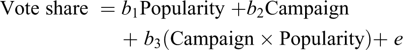
Vote share = b_{1} Popularity + b_{2} Campaign + b_{3} (Campaign \times Popularity) + e

where b ₂ represents overall campaign effectiveness and b ₃ represents variation in effectiveness by the prevailing level of popularity.

To operationalize this, it is also necessary to define popularity. In general terms, popularity refers simply to the existing level of support in the district. However, as district-level opinion polls are relatively rare in Britain as in most countries, it is all but impossible to measure the current level of popularity in a district. We therefore measure popularity by the level of support achieved at the previous election. This has an additional advantage that the term ‘popularity’ is easily understood as the lagged dependent variable in the above equation (see ‘Data and methods’ below).

As noted above, the principle of popularity equilibrium suggests that parties may find it more difficult to increase support where they are already strong because there are fewer new voters to win over. Given that there is a finite amount of support in any constituency, as vote share increases the amount by which a parties’ support can increase further must fall. This is akin to a ceiling effect that gives rise to a compression interaction whereby the size of the effect of the variable of interest (in this case campaign effectiveness) is constrained by the effect of other covariates (popularity) on the outcome (vote share). This is a well-known phenomenon when modelling binary response outcomes and was demonstrated with respect to the impact of registration restrictions on voter turnout, which was found to be greatest for less educated voters who have a lower baseline probability of voting (Nagler, 1991; Wolfinger and Rosenstone, 1980). Countering this compression effect, we might expect that where a party is more popular, there may be a larger pool of potential voters simply because of their popularity. For example, newly eligible voters and incomers may be more likely to support the most popular local party because of neighbourhood effects.

By the same logic, where a party is unpopular (support at the previous election was low), there is a larger pool of voters who could potentially be converted, leading us to expect greater campaign returns in areas of weakness.¹ However, countering this, we might also predict that it is difficult for a party to gain votes where it is very unpopular, for example, because fewer voters in those areas would ever consider voting for a locally unpopular party. If we think of the campaign as affecting the latent utility of voting for a party, rather than simply the binary choice, this implies that the mean latent utility of voters in areas where a party is very weak is lower among the pool of potential recruits than in areas where support is stronger.² Assuming that there is some threshold of utility above which a citizen may vote for a party, then a campaign is less likely to convert an increase in latent utility into actual votes in areas of relative weakness.

The mechanisms we have described suggest countervailing forces which imply that as popularity – measured by previous levels of support – gets very high or very low, then the effectiveness of the campaign will decline. This may be the result of both compression effects caused by the bounded nature of the dependent variable and ‘genuine’ interaction effects (Berry et al., 2010; Rainey, 2016).³ Because of these balancing forces, we predict a curvilinear relationship between campaign effectiveness and previous vote share.

The shape of this curve can be described by its height (i.e. the maximum level of effectiveness), its skewness (the level of previous vote share where we observe maximum effectiveness) and its spread (the extent to which the peak campaign effect and the minimal campaign effect differ from each other). This is represented graphically in Figure 1. In any one given election, for one particular political party, we might expect to find deviations from the general pattern of level, skewness and spread because of variation in the electoral context.

Figure 1.

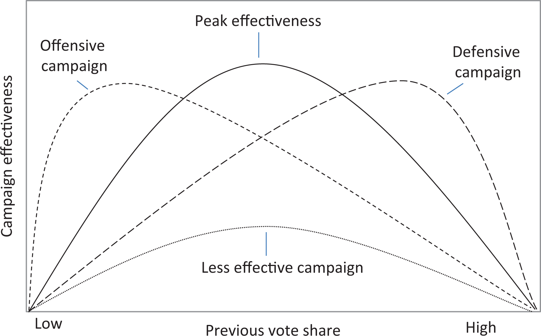
Ideal type of popularity equilibrium.

Perhaps the most important characteristic of the curve is the skewness, indicated by the level of previous vote share at which maximum effectiveness occurs. What this level should be is not immediately obvious. One possible theoretical starting point is that the optimal point should be where the maximum number of electors might potentially vote for a party. This is based on an equivalent principle to that proposed for the maximal effect of GOTV campaigns in promoting turnout at the individual level which, according to Arceneaux and Nickerson (2009), is when voters have a shade under a 0.5 probability of voting. If there were two candidates, 100% turnout and the electorate had normally distributed preferences, this would imply that the maximum point of a curve representing the effectiveness of campaigning by previous vote share would at 50%. However, in the real world, there is no reason to suppose that this should translate to the macro level in such a direct way, especially in a multiparty contest.

While we remain open-minded about the precise location of the inflexion point, we do expect it to vary according to the context of the election and party in question. We propose three main factors that might affect the level of popularity where peak effectiveness is achieved.

First, it will depend on whether a party is on the offensive or a defensive in a particular election campaign. Although the meaning of offensive and defensive is contextually specific, depending on the strategic objectives and expectations of a party, we can make a general definition that helps illuminate the conditions under which the optimal campaign effectiveness will occur. We define an offensive campaign as one where a party has gained popularity since the last election and might expect to target and gain votes and in seats that it does not hold (Fisher et al., 2011). Conversely, we define a defensive campaign as one in which a party has lost support and is targeting voters in seats that it already holds but fears it may lose. Thus, in an election where a party is on the offensive, it should expect to find more potential voters in areas where it is usually relatively weak. In contrast, when a party is on the defensive, it may expect that its usual supporters might require some additional mobilization or persuasion. Because we measure popularity by performance in a previous election, this means that if a party has lost vote share since the last election (and is on the defensive), then its previous vote share will be an overestimation of its underlying popularity (and vice versa). Figure 1 illustrates how the peak of the curve may move depending on whether a campaign is offensive or defensive.

Moreover, if parties achieve synergies from multiple campaign activities (Fieldhouse et al., 2013) or if low level campaign efforts are simply ineffective, then this implies increasing marginal returns to campaigning. In these circumstances, when parties run more offensive campaigns, then their maximum effectiveness will be in districts with lower levels of pre-existing support because this is where they will run their most intensive campaigns (and vice versa). Of course, it is also possible that campaigns may have decreasing marginal returns, for example, if low level campaigns are able to pick the ‘low hanging fruit’. This would also imply that campaign activities would be less effective where campaign intensity is greater, and therefore parties on the defensive would achieve smaller returns on their efforts where they campaign more intensively. Whether marginal returns are increasing or decreasing is tested empirically below.

Second, peak effectiveness will depend on the number of viable candidates or parties competing at the macro level. Under multiparty competition, the effective maximum number of potential votes for any party or candidate is likely to be considerably less than 100%, and thus the peak number of unrealized potential voters is likely to be in areas where support is considerably lower than 50%. This in turn will depend on the distribution of propensities to vote for different parties and how much they overlap. In particular, it will depend on how willing voters are to switch between parties or between voting and non-voting.

Third, the point of maximum effectiveness should be expected to vary by party, and more specifically, according to the macro level of popularity of the party in question. More popular parties tend to retain higher levels of support between elections than smaller parties (Fieldhouse et al., 2019). Moreover, in constituency-based simple plurality systems, smaller parties face the challenge of demonstrating local electoral viability (Russell and Fieldhouse, 2005). As a result, small parties are likely to find it more productive to focus efforts on retaining and building support in areas of existing strength. In other words, they might expect greater electoral returns (or peak effectiveness) in areas where their previous vote share is high.

The other characteristics of the curve in Figure 1 representing the level of campaign effectiveness by previous vote – the spread and the height – may also be context specific. The height of the curve (the overall level of effectiveness) will vary because some parties are simply better at campaigning than others. This is likely to be largely idiosyncratic, although if there are decreasing marginal returns to campaign effort, we would expect that parties that have more extensive campaigns will be less effective (as resources would be more diluted, thereby reducing the intensity of individual campaigns), while parties that have highly targeted and selective campaigns should be more effective, as effort will be better concentrated in those districts that matter most. The spread (or dispersion) represents the extent to which campaign effectiveness varies according to underlying popularity. We have no specific expectation about the degree of variation in campaign effectiveness, although we might expect more distinct peaks (i.e. more variation) when a party or candidate is more selective about where they campaign, and the more effective it is at campaigning overall. This is because, we expect that parties that target their campaigning highly strategically and are more effective should achieve relatively greater returns in those areas where they campaign hardest (i.e. increasing marginal returns). In contrast, less effective and less strategic parties might expect to see similarly low levels of campaign effectiveness everywhere and therefore have flatter curves.

Hypothesis

Based on the theory and discussion, above we propose a general model of popularity equilibrium which states that there will be a curvilinear relationship between the effectiveness of a campaign and the prevailing level of support. The shape of the curve should be a downward parabola (n-shaped). We test the model using data from six elections held between 1992 and 2015 in Great Britain, where robust estimates for campaign intensity are available. Our expectation is that the hypothesized relationship, while affected by the electoral context (e.g. size of constituencies and electoral systems), should be applicable more broadly. However, for the purpose of testing in this specific context, our hypothesis is as follows:

H1: The relationship between campaign effectiveness and previous vote share at the district level will be best described as a downward parabolic (n-shaped) curve.

Data and methods

Because of the availability of a unique longitudinal data set that measures the nature and effectiveness of local campaigns, the case study for testing our theory is Britain, 1992 to 2015. All candidates in British elections are required to have an agent, who is legally responsible for the conduct of the campaign and who is best placed to respond to questions about the local campaign. Data are drawn from surveys of candidates’ electoral agents for the six general elections during this period.⁴ The key variable of interest is the measurement of campaign intensity.

The surveys are specifically designed to measure the level of campaign effort made by local parties in support of candidates at the constituency or district level (Denver and Hands, 1997; Fisher et al., 2011, 2018; Johnston et al., 2011). Over time, campaign methods evolve meaning that a complete measure of campaigning (which captures the wide range of approaches adopted) will not be directly comparable unless it includes only those campaign approaches used in the earliest study. This is unsatisfactory, since the emphasis of campaign techniques shifts over time as technology is adopted, for example. This is a particular concern in our case, as the period under examination is lengthy (23 years), and the technology used in election campaigning has evolved considerably over the period. Indeed, it is worth remembering that in the same year as our first election (1992), Bill Gates predicted that electronic mail might start to ‘catch on’.⁵ To ensure maximum comparability between elections, therefore, we use an index of traditional campaigning originally developed by Fisher and Denver (2008, 2009). This index captures ‘labour intensive’ campaigning that has been widely used in each election and that still accounts for a significant amount of campaign effort (Fieldhouse and Cutts, 2009; Fisher et al., 2011).⁶ These variables capture the number of campaign workers, level of polling day activity, level of doorstep canvassing and the number of leaflets distributed and are used to create scales which are either additive and, where relevant, allow for the size of the electorate in each district. Principal components analysis (PCA) is then used to create an index of traditional campaigning activity. Using conventional cut-off criteria, the PCA suggests one factor is sufficient to represent the variance in the original variables (see Online supplemental appendix). Component scores are then standardized around a mean of 100 for ease of interpretation, which allows comparisons across parties and different years (SD = 34.4, min = 58.0, max = 342.1). Data are pooled across years and parties, not only to maximize sample size (6108 cases), but also to attempt to build a general model of popularity equilibrium, rather than looking at individual elections. The data are unweighted in all analyses, each observation representing a single local campaign.

To preserve comparability over time, we use district-level share of the vote (for each party at each general election) as our dependent variable, for which we have robust estimates across the whole period.⁷ However, this means that if competing parties each mobilize their supporters with equal measures of success in any one district, this will not be reflected in the dependent variable. Nevertheless, if parties differentially increase turnout of their supporters by their own campaign activities, this will be reflected in a higher share of the vote.

To test our hypothesis, we must estimate the effect of campaign effort across different levels of popularity. To operationalize popularity, we require an indicator of the prevailing level local support that can be measured consistently across elections. For reasons discussed above, we therefore use vote share at the previous election (i.e. the lagged dependent variable) which can be measured reliably over time. To test how campaign effectiveness varies with popularity, we also include its interaction with campaign effort. Including the lagged dependent variable also helps in controlling for unobserved factors that are related to both the outcome (vote share) and campaign effort. Moreover, the lagged dependent variable approach is preferable to a change score model for situations where the transient component of Y ₁ (vote at the previous election) is related to X (campaign effort), which we might reasonably expect in this case (Allison, 1990). We also include a squared version of the lagged dependent variable and its interaction with our measure of campaign effort to allow for a curvilinear variation of the effect of campaigning as prior vote share increases. The basic model (without control variables) is therefore represented by the following equation

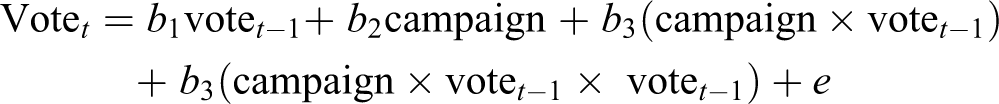
{Vote}_{t} = b_{1} {vote}_{t - 1} + b_{2} campaign + b_{3} (campaign \times {vote}_{t - 1}) + b_{3} (campaign \times {vote}_{t - 1} \times {vote}_{t - 1}) + e

where the effectiveness of the campaign is measured by the average marginal effect of campaign effort (Berry et al., 2010; Rainey, 2016).

In addition to the basic model, to allow for the possible impact of opposing party campaigns, we control for the total amount of campaign spending by each of the other parties competing in the constituency.⁸ This is important because parties tend to compete with each other in marginal seats (Fieldhouse and Cutts, 2009; Fisher et al., 2011) and part of the effect of a party’s efforts may be offset by that of opposing parties. For example, additional campaign effort in a marginal and highly competitive seat may have less impact than the equivalent amount of effort in a very similar seat where other parties are hardly campaigning. Although spending is a less good measure of campaign effort than that derived from the survey, it provides a reliable proxy (Fieldhouse and Cutts, 2009). It also ensures that there are measures of opposing campaigns in every constituency for which we have campaign–survey data for any one of our three parties under analysis.

We also control for candidate incumbency to allow for the exogenous effect of the boost enjoyed by personal incumbents. Personal incumbency has been shown to have a positive impact on vote share which can be enhanced through personalized campaigns – a trend observable across a number of different countries (e.g. Denver and Hands, 1997; Gschwend and Zittel, 2015). To allow for variations in party fortunes between elections, we control for the specific election year as a fixed effect. Finally, we control for country (England, Scotland or Wales) to reflect the fact that in Scotland and Wales, the existence of nationalist parties (Plaid Cymru in Wales and the Scottish National Party in Scotland) means viable choice sets tend to be larger and vote share of the major parties is affected accordingly.⁹ Party dummies are included to adjust for the fact that different parties get different shares of votes. Party by election year interactions are required to allow for variation in support for each party by election. We model vote shares for Conservatives, Labour and the Liberal Democrats, the three largest parties competing across Britain over the six elections analysed.

Modelling vote shares expressed as a percentage can be problematic because predicted values of Y can fall outside of the range zero to one hundred. When modelled using ordinary least squares (OLS) regression, our data reveal heteroscedasticity and a small proportion of negative predicted values. While transformations such as the logit can provide a solution to this, a more flexible and appropriate approach is beta regression. Beta regression is a type of regression model suitable for situations in which the response is continuous, bounded by zero and one and beta distributed (Ferrari and Cribari-Neto, 2004). The beta distribution is defined by two parameters representing the mean and variance of the response, making the model sufficiently flexible to handle a variety of situations. The model allows for asymmetry in proportions and facilitates interpretation of coefficients on the original scale. Before modelling, vote share is divided by 100 to ensure that it lies between 0 and 1 as required by beta regression.

Beta regression is a model of the mean of the dependent variable y conditional on covariates x denoted as $E (y / x) = µ x$ .

If we observe response data Y _1… on (0, 1), then the beta regression model assumes that the mean of these random variables can be represented as follows

g (µ_{i}) = η_{i} = β_{0} + β_{1} X_{i 1}

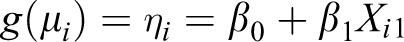
where the logit link function g(·) in a beta regression maps the response variable observed (y ₁) on the interval (0, 1) to the real line. The analysis is implemented with Stata 14 Betareg command.

Results

Table 1 shows the coefficients for the pooled model for all years and parties. As hypothesized, there are significant effects for campaign effort (as captured by the traditional campaign index) and its interaction with vote share at the previous election. The squared term for previous vote share is significant but the interaction of the squared term and campaign effort is not significant. There is also a significant main effect for prior vote share and as well as significant effects for opposing campaign spending, incumbency, country and year. All are in the direction expected. A number of the year-by-party interactions are also significant, reflecting how different parties performed in various elections.

Table 1.

Pooled years beta regression of vote share divided by 100.

	Coefficient	Standard error
Incumbent candidate	0.076**	(0.008)
Opposition spend	−0.001**	(0.000)
Campaign effort	0.006**	(0.001)
Vote share t − 1	0.072**	(0.003)
effort # vote share t − 1	−0.000**	(0.000)
Vote share t − 1 # vote share t−1	−0.000**	(0.000)
effort # vote share t − 1 # vote share t − 1	−0.000	(0.000)
Country (ref = England)
Wales	−0.024*	(0.012)
Scotland	−0.053**	(0.011)
Party (ref = Conservative)
Labour	0.183**	(0.017)
Liberal Democrat	−0.252**	(0.018)
Year (ref = 1992)
1997	−0.468**	(0.016)
2001	0.018	(0.017)
2005	−0.006	(0.026)
2010	0.146**	(0.018)
2015	0.043*	(0.018)
Party by year
Labour # 1997	0.728**	(0.021)
Labour # 2001	−0.208**	(0.023)
Labour # 2005	−0.388**	(0.031)
Labour # 2010	−0.619**	(0.024)
Labour # 2015	−0.184**	(0.024)
Liberal Democrat # 1997	0.619**	(0.024)
Liberal Democrat # 2001	0.315**	(0.024)
Liberal Democrat # 2005	0.480**	(0.033)
Liberal Democrat # 2010	0.192**	(0.025)
Liberal Democrat # 2015	−1.043**	(0.029)
Constant	−2.998**	(0.051)
Scale
Constant	4.75**	(0.018)
Observations	6104

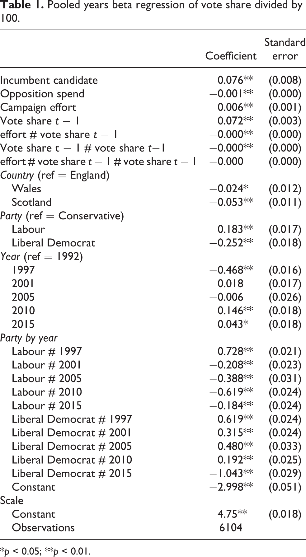
*p < 0.05; **p < 0.01.

To interpret the effect of campaigns on vote share across all six elections, we can look at the predictive margins of vote share for any given value of campaign effort, conditional on all other variables in the model. Overall, the average marginal effect of campaign effort across all parties and year is 0.044 or nearly half a percentage point increase in vote share for every 10 points increase in campaign effort. This means that, other things being equal, in a constituency where the campaign effort was 200, the expected vote share would be approximately 9 percentage points higher than where the campaign effort was zero. More modestly, an increase in campaign effort of one standard deviation (34 points) from its mean of 100 gives rise to a 1.7% increase in vote share. This is consistent with previous research on individual British elections which shows that local campaigns have a positive impact on vote share (Fieldhouse and Cutts, 2009; Fisher and Denver, 2009; Fisher et al., 2016; Johnston et al., 2011).

The theory of popularity equilibrium for campaign effects implies that, at some levels of existing popularity, campaigns will have more effect than at others. We can observe this by visualizing the predictive margins conditional on alterative values of prior vote share. Figure 2 shows the equivalent relationship where vote share in the previous election was 20%, 40% and 60%. We observe that when prior vote share is 40%, we see a positive relationship and a difference of around 9 percentage points as we move from the least to most intense campaigns. When prior vote share is much higher (60%), the effect flattens off, providing evidence of the hypothesized ceiling effect. However, there is no evidence of a floor effect. When previous vote share is 20%, the gradient actually appears a little steeper than at 40%.

Figure 2.

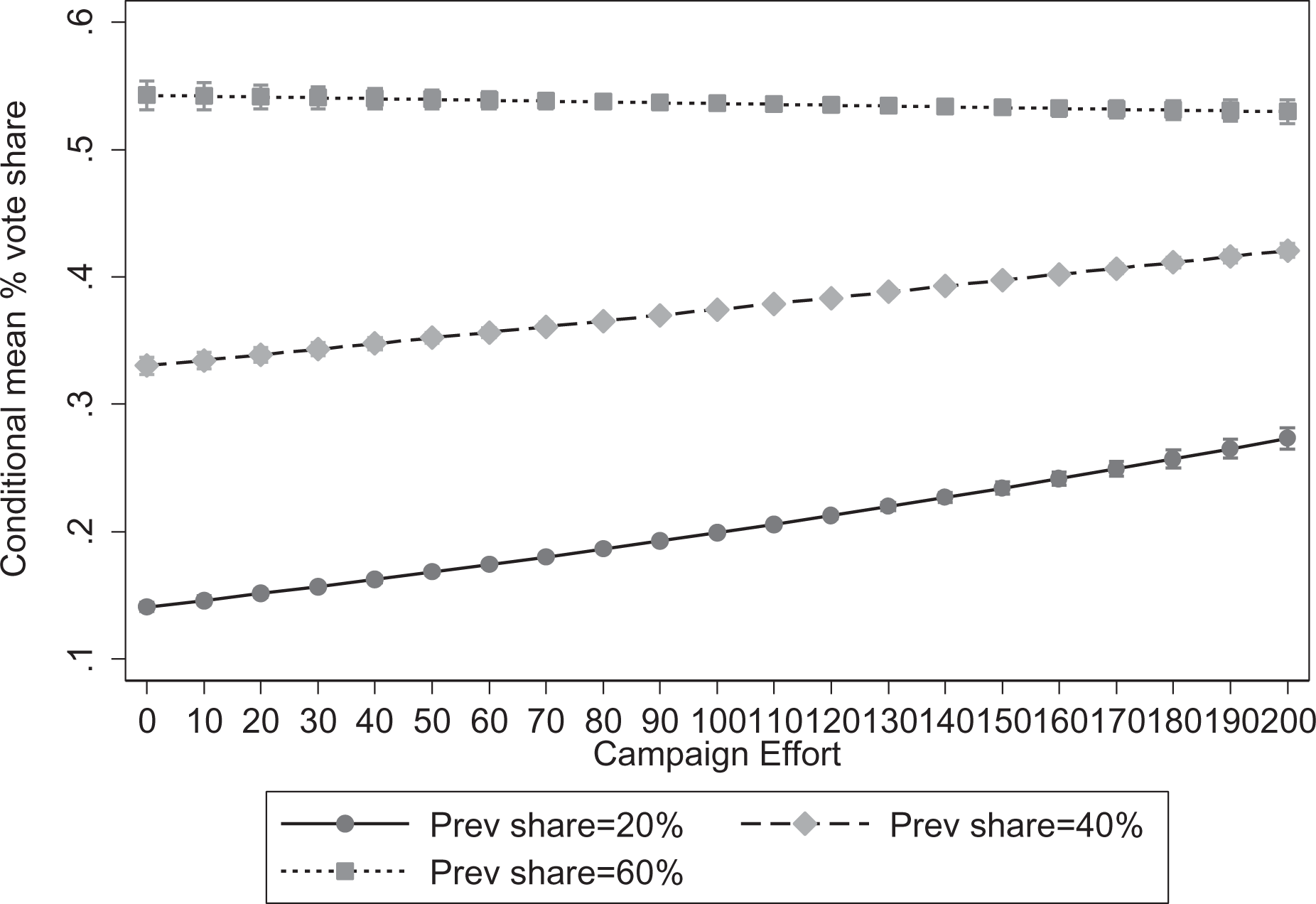
Predictive margins by campaign effort and previous vote.

To demonstrate this systematically, Figure 3 shows the average marginal effect of a unit change in effort (i.e. the first derivative, dy/dx) by the level of prior vote share. In other words, this represents the level of campaign effectiveness by the level of underlying support. Figure 3 confirms the parabolic relationship between campaign effectiveness and previous vote share that was predicted by the general model of popularity equilibrium. A reduced form of the model is shown in the Online supplemental appendix Figure A1 and reveals an almost identical parabola, indicating that while the controls may remove some anomalies and improve model fit, the general model of popularity equilibrium holds regardless of these additional intervening factors.

Figure 3.

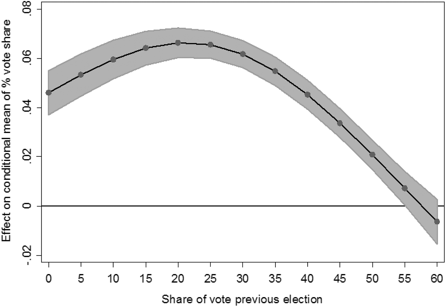
Average marginal effects of campaign on vote share by previous vote share.

Figure 3 also shows that at the optimal level of prior vote share, for each one point change in campaign effort, a party can expect an increase in vote share of 0.07%. This equates to an increase in vote share of approximately 2.3% for a one standard deviation increase in campaign effort. This campaign peak effect occurs where prior vote share is approximately 23%.¹⁰ The shape of the curve suggests that there is a floor effect but it is manifest only at a very low level of prior popularity. This suggests that gaining additional votes in areas where a party vote share is already high is more expensive in terms of campaign effort than in areas where there are more voters ‘up-for-grabs’. When prior vote share exceeds 60%, campaigning appears, on average, to be completely ineffectual and may even be associated with worse performance. This may seem odd at first sight, but it is entirely possible the campaigning by a locally dominant party might antagonize opposition voters, raising turnout of supporters of other parties. That is electors who oppose the likely winner may be motivated to vote for expressive reasons if the dominant party increases its visibility. There is empirical evidence that under certain conditions or where certain campaign methods are employed, a party’s campaigns can also depress turnout (Fisher et al., 2016; Gerber and Green, 2000; Green and Gerber, 2004; Morisi, 2018).

What is clear from Figure 3 is that there is strong evidence of the curvilinear relationship between prevailing support and campaign effectiveness as described by the general model of popularity equilibrium and its impact on campaign effectiveness. As noted above, the effectiveness of a campaign will vary from year to year and party to party. To assess, therefore, how far individual campaigns vary from the usual pattern, in the following section, we examine how the model varies between parties and elections.

Variation between elections and parties

So far, we have laid out the evidence in support of our hypothesis using pooled data spanning thousands of district-level observations from six elections over the course of 23 years and three parties. However, as discussed above, we expect that the nature of the relationship between local popularity and local campaign effectiveness will vary by party and election for several reasons, including the average level of campaign effectiveness of a party; whether it is on the offensive or defensive; and its macro (national) level of popularity.

With respect to the level of campaign effectiveness, previous research has demonstrated that in Britain some parties’ campaigns are more effective than others This reflects party level factors including how well campaigns are managed and coordinated nationally, the clarity of objectives and the ability to strategically target campaign resources in key districts (Fisher et al., 2011, 2018; Fisher et al., 2006). Our modelling over six elections confirms previous research from single elections in Britain, which show that, of the three main parties under consideration, the Conservatives, on average, run the least effective local campaigns and the Liberal Democrats the most effective (Denver and Hands, 1997; Fisher et al., 2011). Fitting the same model shown in Table 1 separately for each party (across all elections), we find an average marginal effect of campaign effort for the Conservatives of 0.01, for Labour of 0.04 and the Liberal Democrats of 0.06. We also know that, for the time period under consideration, the Liberal Democrat vote share has been consistently lower than that of the two major parties. Moreover, the Liberal Democrats also have the lowest average level of campaign effort over the period (84) compared to Conservatives 115 and Labour 105. With this information in mind, we redraw the campaign effectiveness curve shown in Figure 3 based on the three party specific models. The three curves are displayed in Figure 4 with a reference line on the x-axis at 23% to illustrate deviation from the average pattern.¹¹

Figure 4.

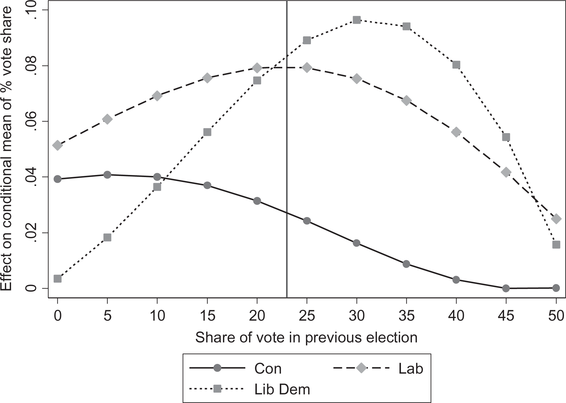
Average marginal effects of campaign on vote share by previous vote share modelled separately by party.

Figure 4 confirms that Conservative campaigns are, on average, less effective than those of Labour or the Liberal Democrats. The curve is flatter and lower, with a less obvious peak as we expect for a less effective campaigning party (see above). The Conservative peak is found where their vote share is low, declining as vote share increases. This is in keeping with the fact that for most of this period, the Conservatives have not acted especially strategically in their local campaigning, expending a lot of effort simply where they have the resources (Fieldhouse and Cutts, 2009). This has been, in part, because of the relative independence of the party’s constituency associations from the central party (Fisher and Denver, 2008). That said, the level of variation is not great, ranging between 0 and 0.04%. Figure 4 also reveals the Liberal Democrats’ campaigns to be the polar, the opposite of the Conservatives’. As the party with the lowest average level of campaign effort and the lowest average vote share, they are also the most selective, targeting areas of existing strength. The Liberal Democrats have traditionally been a party highly dependent on grassroots campaigning and have run their most effective campaigns in areas of established strength where they are regarded as electorally viable (Russell and Fieldhouse, 2005). This is reflected in a curve with more negative skew than the other parties, and high maximum points of almost 0.1 (a difference of 10% points of vote share between a district with 0 campaign effort and 1 with 100). Finally Labour’s campaign effectiveness conforms most closely to the ideal type shown in Figure 1 and the general model shown in Figure 3, with a peak around 23%.

Although Figure 4 illustrates very clearly how the general model of popularity equilibrium can vary by party, this does conceal considerable variation over time. By disaggregating our models further, fitting equivalent models for each party at each election, we are able to observe such variation. Figure 5 provides illustrations of the results of such models. Each panel shows the average marginal effect of campaign effort by previous vote share, as in Figures 3 and 4. This illustrates that the relationship between party vote share and campaign effectiveness does vary somewhat for each party in each election. Consistent with our expectation about offensive and defensive campaigns, Figure 5 suggests that the largest differences occur when a party experienced a dramatic change of fortune between elections, such as the Conservatives in 1997 (when Labour won a landslide) and the Liberal Democrats in 2015 (when the party’s vote share fell by 15.5 percentage points).

Figure 5.

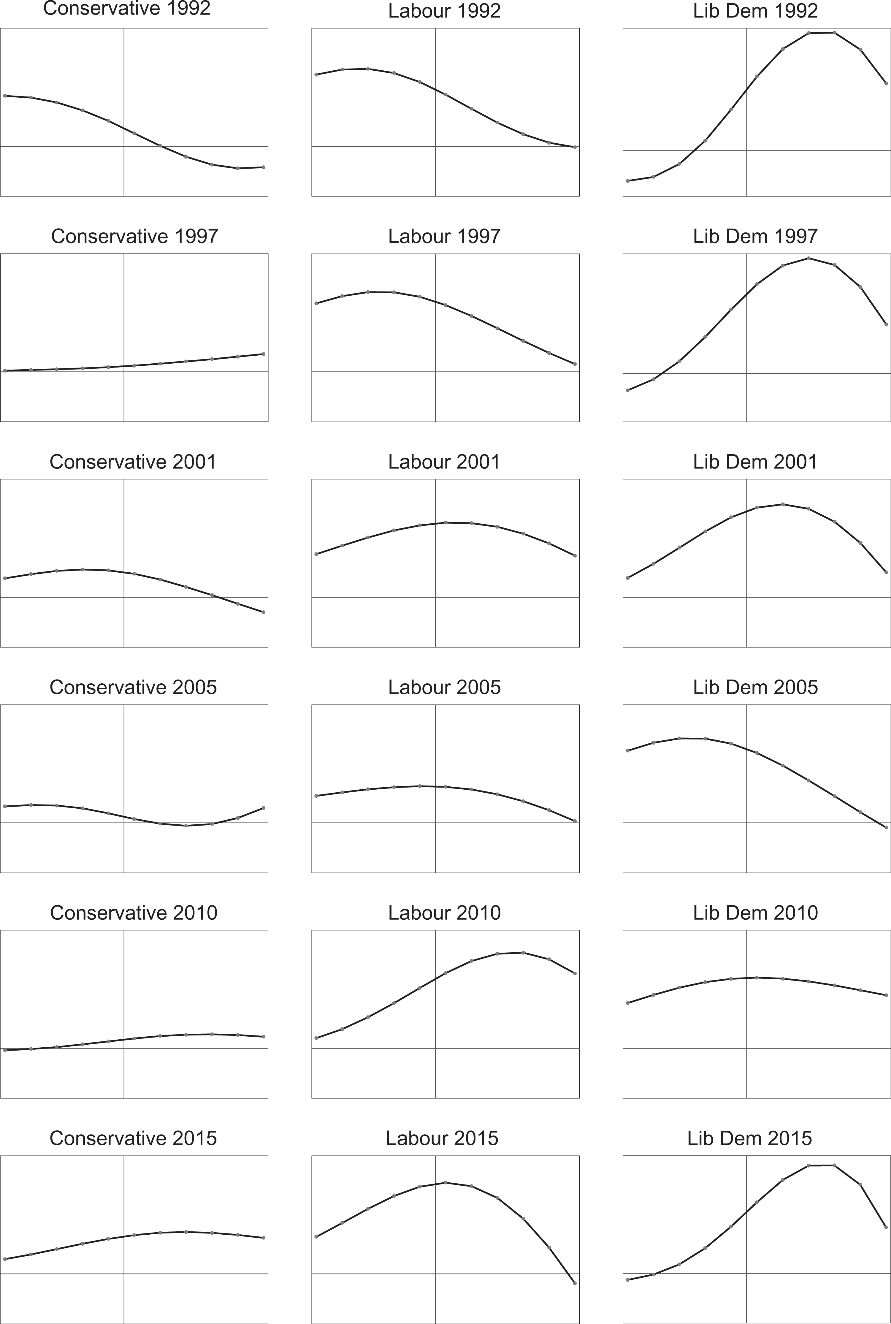
Average marginal effects of campaign on vote share by previous vote share modelled by party and election. Note: All charts have the same scale, y-axis running from a maximum campaign effect of −0.04% to 0.10% with a reference line at zero; and x-axis running from previous vote share 0% to 50%, with a reference line at 23%.

We have already described the general character of Conservative campaign effectiveness, and this is repeated across elections: the curves are, for the most part, lower than the other parties, positively skewed and relatively flat. Indeed, in all but two elections (1997 and 2015), the overall average marginal effect for the Conservative campaign was not significantly greater than zero. As in Figure 4, the Liberal Democrat election specific curves are characterized by more negative skew than the other parties (representing greater effectiveness where previous support is higher) and high maximum points, except in 2005 and 2010 when their effectiveness was more evenly spread, in elections in which they ran more offensive campaigns (Fisher et al., 2011). In 2015, following a period in coalition government which drastically affected their popularity, the Liberal Democrat campaign was, again, most effective in areas of pre-existing strength, returning to the pre-2005 pattern. As discussed above, this is typical of what we would expect for a defensive campaign strategy. The pattern of effectiveness demonstrated for the Liberal Democrats is an indicative of a well-coordinated and effective campaign insofar as peak effectiveness is at a reasonably high level of support (around 30–35%) where increasing vote share is both more difficult (for reasons explained above) but more useful (as it is more likely to influence the outcome).

Finally, as shown in Figure 4, Labour plots are more in line with the ideal type with quite distinct curves and maximum points varying. These reflect both the degree of effective targeting and also the change in popularity (captured by vote share) from election to election. The least distinctive peak and least effective district-level campaigns were in 2005 when Labour was re-elected as the governing party but with a reduced vote share.

In general, as anticipated, we find that when parties are on the offensive (when their national vote share has increased since the previous election), the curves tend to be characterized by positive skew as parties perform better and get more reward by campaigning in areas outside of their existing strongholds. More defensive campaigns are characterized by negative skew as parties are more successful at shoring up support in their heartlands. Labour in 2010 illustrates a good example of a defensive campaign where maximum effectiveness was in safer seats (helping to deny the Conservatives a majority in that election – see Fisher et al., 2011), while the curve for 1997 reflects an offensive campaign, which was most effective in seats with previously low levels of support, helping to deliver a landslide for Labour.

Overall, what is important is that while our pooled analysis (illustrated in Figure 3) supports the general model of popularity equilibrium, the disaggregated analyses in Figure 5 illustrate the degree of deviation from the general model for any one party in any one year as a result of variations in context. Fundamentally, however, it is also apparent that our general model of popularity equilibrium is applicable over time. While shape of the curve may deviate in any one year for any one party, the principle of popularity equilibrium does not – the effectiveness of parties’ campaigns is a function, in part, of that party’s local level of popularity.

Explaining variation

As discussed above, there are several reasons why the overall level of performance of the party and whether it is on the offensive or defensive at a particular election may affect the shape of the curve. The first relates to the operationalization of local (underlying) popularity: if a party has lost support since the previous election, then previous vote share will overestimate the underlying level of popularity in the constituency, shifting the maximum point of the curve to the right (or vice versa for parties that have gained support). Second, when a party is on the offensive, it should expect to find more potential voters in areas where it is usually relatively weak (and vice versa). Third, if there are increasing marginal returns to campaign effort, campaign effectiveness will be higher when effort levels are greater. This is investigated in Figure 6, which shows how the marginal effect of effort on vote share varies according to the level of campaign effort level. It shows how the gradient of the curve displayed in Figure 3 changes with the level of campaign effort – that is, its second derivative. We see a positive relationship between the level of campaign effort and its marginal effectiveness indicating increasing marginal returns.¹² This also implies that greater campaign effectiveness should be achieved in the types of area where parties campaign intensively including marginal constituencies (notwithstanding the counter-effect of opposing campaigns). Partly as a result of these increasing marginal returns, in elections when parties run more offensive campaigns, their maximum effort and maximum effectiveness tend to be in districts with lower levels of pre-existing support. In more defensive campaigns, maximum effectiveness tends to be in seats with higher levels of prior support.

Figure 6.

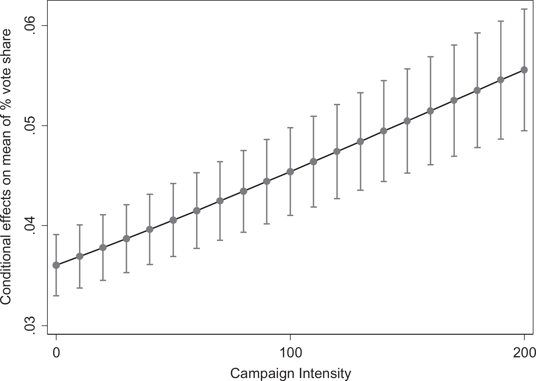
Increasing marginal returns: the average marginal effects of campaign effort on vote share by level of effort.

We can illustrate the systematic relationship between the point of peak effectiveness and the degree to which a party is on the offensive or defensive by plotting the peak effectiveness derived from the predictive margins of the disaggregated models shown in Figure 6 and the change in macro vote share of the party in question since the last election (Figure 7). A party that is losing support can be thought of as being on the defensive, while a party whose support is increasing is on the offensive. Figure 7 shows a strong negative relationship between the point of maximum effectiveness and change in vote share, with the parties gaining most ground having their peaks at the lowest levels of prior support (e.g. Labour in 1997) and parties on the defensive having peaks at high levels of prior support (e.g. Liberal Democrats in 2015 and Conservatives in 1997).

Figure 7.

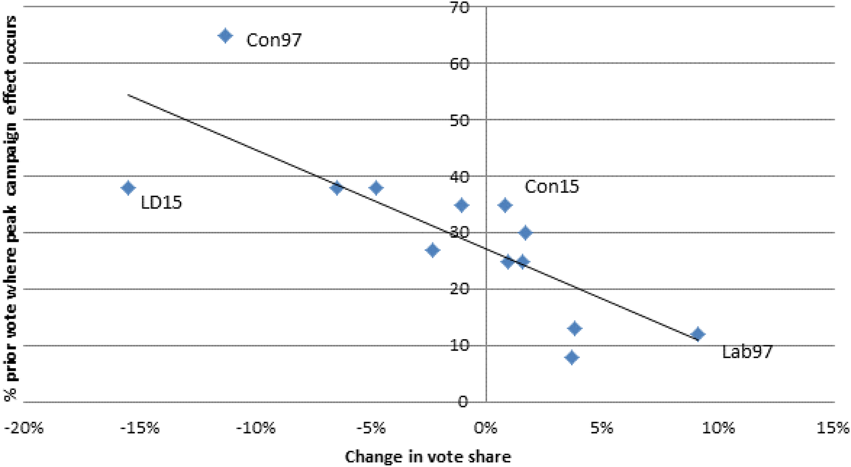
Point of maximum campaign effectiveness by macro change in vote share since last election. Note: Points represent inflexion point of charts in Figure 6, excluding cases where the overall average marginal effect is not significant. Excluded cases are Conservative 1992, 2001, 2005, 2010 and Labour 2005. Reference line is linear best fit (R ² = 0.62).

Conclusions

In this article, we have advanced a general theory of campaign effectiveness that is a curvilinear function of underlying popularity (measured here by vote share). Whether we include extensive control variables or not, our analyses point to the same conclusion: the effectiveness of campaign effort is greatest where the level of existing support is neither very low nor very high. This is consistent with the concept of a popularity equilibrium (Fisher et al., 2011). This article has introduced and tested a theory of local campaign effectiveness that holds for parties or candidates across elections. Unlike previous research on campaign effectiveness – for example, much of the literature on GOTV – it focuses on the characteristics of the district rather than the characteristics of individual voters, providing insight into where local campaigns are more or less effective.

In the context of the data used to test this theory, the model indicates that the optimal point of underlying support (approximately 23%) is lower than the typical level of support that is required to win a seat in British Elections.¹³ The lesson more generally is that in a multiparty system where numerous parties are competing over votes, the most fertile ground for campaign effort is not in hopeless seats or safe seats but in areas that parties need to improve their vote share by a substantial amount to gain representation. However, the effort required to win additional votes rises quite sharply as we move towards 40% of the vote. Winning additional votes in both safe seats and areas of extreme electoral weakness tends to be substantially more difficult. It is important to remember that this is an aggregate level theory concerned with characteristics of constituencies and the relative ease or difficulty of the task faced by campaigners in constituencies with different levels of popularity. It is therefore appropriate that this has been tested with aggregate (constituency) level data. Further research using individual level data could help to identify what is different about voters in the areas identified as more or less productive for campaigners.¹⁴

The optimal point of effectiveness at a little over 20% is rather lower than the level which would be strategically most advantageous for campaigners. While, it is clear that the availability of reservoirs of untapped support is particularly important in campaign effectiveness, it is unlikely that gaining additional votes in constituencies where existing support is much less than 30% would deliver additional seats in Parliament. Although it is more difficult for campaigns to deliver increased vote share when existing support exceeds 25–30%, it is in these areas where votes have the most value for winning seats. The ability of parties to achieve that depends on the quality of their national coordination and targeting strategies. We have found that the Liberal Democrats tend to have peak effectiveness at rather higher levels than the other parties, especially the Conservatives, which helps illuminate why previous research has consistently shown them to have more effective campaigns.

As well as testing a general model of local campaign effectiveness we have set out theoretical reasons for variation in effectiveness and, where possible, tested those explanations. With respect to the point of peak campaign effectiveness, we have suggested three factors. The first was the number of viable parties at the macro level. Under multiparty systems, we might expect to find a party’s greatest potential support base where previous support is relatively low compared to a classic or very dominant two party system. We are currently unable to test this outside of the context of British Elections (for which we have the relevant campaign effort data) but should be the focus on further research. Second, the location of the peak reflects the underlying level of popularity of the party. We found evidence consistent with this insofar as the two major parties had positively skewed peaks while the Liberal Democrats had a negatively skewed peak. Third, and most importantly, the position of the peak depends on whether a party is on the offensive or defensive at any given election. We show that parties running more offensive campaigns enjoy greater campaign effectiveness in areas of lower previous vote share (i.e. curves with positive skew); while less popular parties (and defensive campaigns) are more effective in areas of existing strength (negative skew).

We believe these findings have crucial implications for scholarly understanding of district-level campaign effects. But in practical terms, how does this help candidates and parties know where to focus their campaigns? Candidates and parties are generally interested in winning seats and are therefore unlikely to campaign more in an area simply because the returns will be greater. However, we suggest two reasons why this information is valuable to campaigners. First, not all campaigns are exclusively about winning seats but about winning vote share. Although the theory is tested in the context of a first-past-the-post system, there is no reason that the same general model of popularity equilibrium should not apply in proportional systems where vote share may be crucial, especially as comparative research shows that electoral systems have little impact on the effectiveness of district-level campaigning (Gschwend and Zittel, 2015; Karp et al., 2008). Moreover, even in simple plurality systems, there are many reasons that parties may be interested in maximizing vote share, not least to build credibility in a greater range of districts to build a platform for future elections, whether first or second order. Second, understanding where campaigns are more or less effective allows campaigners to judge the amount of effort required to change the outcome of a district vote. Gerber and Green (2004) provide guidance on how campaigners can estimate the cost of winning each extra vote. Our research provides a mechanism for calibrating the cost or effort according to prior levels of support. For example, the general model implies that it will require much more effort to increase vote share from 35% to 40% (often a crucial improvement required to win a seat) compared to increasing vote share from 25% to 30%. While further research is required to more finely calibrate how the general model of popularity equilibrium impacts on campaign effectiveness in a variety of different electoral contexts, by examining the intensity of campaigns in over 6000 electoral contexts in six different general elections, we have established that, as far as local campaigns go, the three bears in Goldilocks had the right idea: the local electorate should neither be too cold nor too hot but just right.

Supplemental Material

Supplemental Material, sj-pdf-1-ppq-10.1177_1354068818823443 - Popularity equilibrium: Testing a general theory of local campaign effectiveness

Supplemental Material, sj-pdf-1-ppq-10.1177_1354068818823443 for Popularity equilibrium: Testing a general theory of local campaign effectiveness by Edward Fieldhouse, Justin Fisher and David Cutts in Party Politics

Footnotes

Declaration of Conflicting Interests

The authors declared no potential conflicts of interest with respect to the research, authorship, and/or publication of this article.

Funding

The authors disclosed receipt of the following financial support for the research, authorship, and/or publication of this article: This research was supported by the Economic and Social Research Council, grant number ES/M007251/1.

ORCID iD

Edward Fieldhouse

Supplemental Material

Supplemental material for this article is available online.

Notes

References

Allison

(1990) Change scores as dependent variables in regression analysis [online]. Sociological Methodology 20: 93. Available at: http://www.jstor.org/stable/271083?origin=crossref (accessed 3 January 2019).

Arceneaux

Nickerson

(2009) Who is mobilized to vote? A re-analysis of 11 field experiments [online]. Source: American Journal of Political Science 5359124(1): 1–16. Blackwell Publishing Inc. DOI: 10.1111/j.1540-5907.2008.00354.x.

Berry

DeMeritt

JHR

Esarey

(2010) Testing for interaction in binary logit and probit models: is a product term essential? [online]. American Journal of Political Science 54(1): 248–266. Wiley/Blackwell (10.1111). DOI: 10.1111/j.1540-5907.2009.00429.x.

Denver

Hands

(1997) Modern Constituency Electioneering: Local Campaigning in the 1992 General Election. London: F. Cass.

Ferrari

SLP

Cribari-Neto

(2004) Beta regression for modelling rates and proportions. Journal of Applied Statistics 31(7): 799–815.

Fieldhouse

Cutts

(2009) The effectiveness of local party campaigns in 2005: combining evidence from campaign spending and agent survey data. British Journal of Political Science 39(2): 367–388.

Fieldhouse

Cutts

John

, et al. (2014) When context matters: assessing geographical heterogeneity of get-out-the-vote treatment effects using a population based field experiment. Political Behavior 36(1): 77–97.

Fieldhouse

Cutts

Widdop

, et al. (2013) Do impersonal mobilisation methods work? Evidence from a nationwide get-out-the-vote experiment in England. Electoral Studies 32(1): 113–123.

Fieldhouse

Green

Evans

, et al. (2019) Electoral Shocks: The Volatile Voter in a Turbulent World. Oxford University Press.

10.

Fisher

(2000) Small kingdoms and crumbling organizations: examining the variation in constituency party members and resources. British Election and Parties Review 10(1): 133–150.

11.

Fisher

Cutts

Fieldhouse

(2011) The electoral effectiveness of constituency campaigning in the 2010 British general election: the “triumph” of Labour? Electoral Studies 30(4): 816–828. Pergamon.

12.

Fisher

Cutts

Fieldhouse

, et al. (2018) The impact of electoral context on the electoral effectiveness of district-level campaigning: popularity equilibrium and the case of the 2015 british general election [online]. Political Studies, 1–20. DOI: 10.1177/0032321718764800.

13.

Fisher

Denver

(2008) From foot-slogging to call centres and direct mail: a framework for analysing the development of district-level campaigning. European Journal of Political Research 47(6): 794–826.

14.

Fisher

Denver

(2009) Evaluating the electoral effects of traditional and modern modes of constituency campaigning in Britain 1992–2005. Parliamentary Affairs 62(2): 196–210.

15.

Fisher

Denver

Hands

(2006) The relative electoral impact of central party co-ordination and size of party membership at constituency level [online]. Electoral Studies 25(4): 664–676. Pergamon. Available at: https://www-sciencedirect-com.manchester.idm.oclc.org/science/article/pii/S0261379405000922 (accessed 3 January 2019).

16.

Fisher

Fieldhouse

Johnston

, et al. (2016) Is all campaigning equally positive? The impact of district level campaigning on voter turnout at the 2010 British general election. Party Politics 22(2): 215–226.

17.

Gerber

Green

(2000) The effect of a nonpartisan get-out-the-vote drive: an experimental study of leafletting. Journal of Politics 62(3): 846–857.

18.

Green

. (2004) Mobilizing African-American voters using direct mail and commercial phone banks: a field experiment [online]. Political Research Quarterly 57(2): 245–255. SAGE Publications Sage CA: Thousand Oaks, CA.

19.

Green

Gerber

(2004) Get Out the Vote : How to Increase Voter Turnout. Washington DC: The Brookings Institution.

20.

Gschwend

Zittel

(2015) Do constituency candidates matter in German Federal Elections? The personal vote as an interactive process. Electoral Studies 39: 338–349. Pergamon.

21.

Hillygus

(2005, February 1) Campaign effects and the dynamics of turnout intention in election 2000. Journal of Politics 67:50–68. Blackwell.

22.

Johnston

Pattie

Cutts

, et al. (2011) Local campaign spending at the 2010 general election and its impact: exploring what wider regulation has revealed. Political Quarterly 82(2): 169–192.

23.

Karp

Banducci

Bowler

(2008) Getting out the vote: party mobilization in a comparative perspective. British Journal of Political Science 38(01): 91–112. Cambridge University Press.

24.

Kramer

(1970) The effects of precinct-level canvassing on voter behavior. Public Opinion Quarterly 34(4): 560. Oxford University Press.

25.

Morisi

(2018) When campaigns can backfire: national identities and support for parties in the 2015 U.K. General election in Scotland [online]. Political Research Quarterly 71: 895–909. SAGE Publications Sage CA: Los Angeles, CA. DOI: 10.1177/1065912918771529.

26.

Nagler

(1991) The effect of registration laws and education on U.S. Voter turnout [online]. The American Political Science Review 85(4): 1393. Available at: http://www.jstor.org/stable/1963952?origin=crossref (accessed 3 January 2019).

27.

Niven

(2001) The limits of mobilization: turnout evidence from state house primaries. Political Behavior 23(4): 335–350. Kluwer Academic Publishers-Plenum Publishers.

28.

Norris

(2006) Did the media matter? Agenda-setting, persuasion and mobilization effects in the british general election campaign. British Politics 1(2): 195–221. Palgrave Macmillan UK.

29.

Rainey

(2016) Compression and conditional effects: a product term is essential when using logistic regression to test for interaction [online]. Political Science Research and Methods 4(03): 621–639. Available at: http://www.journals.cambridge.org/abstract_S204984701500059X (accessed 3 January 2019).

30.

Rosenstone

Hansen

(1993) Mobilization, Participation, and Democracy in America. New York: Macmillan.

31.

Russell

Fieldhouse

(2005) Neither Left Nor Right: The Liberal Democrats and the Electorate. Manchester: Manchester University Press.

32.

van der Eijk

van der Brug

Kroh

, et al. (2006) Rethinking the dependent variable in voting behavior: on the measurement and analysis of electoral utilities. Electoral Studies 25(3): 424–447.

33.

Wolfinger

Rosenstone

(1980) Who Votes? New Haven: Yale University Press.

Supplementary Material

Please find the following supplemental material available below.

For Open Access articles published under a Creative Commons License, all supplemental material carries the same license as the article it is associated with.

For non-Open Access articles published, all supplemental material carries a non-exclusive license, and permission requests for re-use of supplemental material or any part of supplemental material shall be sent directly to the copyright owner as specified in the copyright notice associated with the article.

0.00 MB

0.27 MB