
Abstract
The in situ measurement of acoustic surfaces presents a significant challenge in room acoustics, as it is often impractical to conduct laboratory measurements of already installed materials. In a former study, the in situ analysis of porous samples that react locally when supported by a solid wall demonstrated a good degree of accuracy. Nevertheless, when a porous layer is supported by a large air cavity (depth >100 mm), a situation commonly seen in suspended ceiling designs, the air cavity exhibits a non-locally reacting behavior; thus, the local reaction cannot be reliably assumed. This study introduces a method to characterize such a non-locally responding system through in situ PU probe measurements, utilizing an inverse technique to fit the parameters of the impedance model of a porous layer that is backed by an infinite air layer, based on the measured reflection coefficient. The precision of the approach was confirmed through 2D numerical simulations, indicating that the method produced reliable results for air cavities of 200 mm or deeper. The method was then experimentally validated on systems comprising several porous layers supported by air cavities of varying depths. Good agreement was obtained between the parameters measured experimentally using the proposed technique and the references, even in cases where the air cavity was less than 200 mm deep. Additionally, the proposed method demonstrated more precise characterization results compared to those achieved by fitting the parameters of an impedance model based on a standard multilayer model.
Keywords
Introduction
A frequent challenge in room acoustic consultancy is accurately assessing the acoustic characteristics of materials present in a pre-existing space. This is particularly important when performing an acoustic simulation for that space, as the precision of the material properties inputted significantly impacts the simulation’s accuracy. 1 In such scenarios, it is often not feasible to extract a material sample for laboratory assessment, such as with the impedance tube method. Additionally, even if a product sample is available from the manufacturer for laboratory tests, factors like the conditions of installation and wear over time can influence the acoustic properties, highlighting the necessity for an on-site evaluation.
A considerable amount of research has focused on in situ measurement and free-field techniques for assessing material characteristics. Numerous approaches have been compiled in a review of in situ and free-field measurement methods by Brandão et al. 2 Contrary to this review, the term “in situ measurements” in this paper refers specifically to free-field measurement methods applied in the field (i.e. not in anechoic or semi-anechoic conditions). Additionally, there are more recent studies available in the literature.3 –8 In a prior publication, it was demonstrated that the combination of a pressure and velocity (PU) in situ measurement approach with model fitting optimization enabled rapid and precise characterization of a locally reacting porous material supported by a hard surface. 9 Other studies have explored the capabilities of pressure-velocity sensors for evaluating the acoustical properties of porous materials that are backed by a hard surface, including research by Tijs et al., 10 Sakamoto et al., 11 and Van Hoorikx et al. 12 This research investigates the suitability of this approach when applied to another common acoustic systems involving a porous layer.
Porous layers backed by a large air cavity are common sound–absorbing systems and their configuration poses a challenge to applying the in situ characterization proposed in this previous publication. 13 A common example of such a system is a suspended ceiling, with a large air cavity (100–500 mm) above the layer. In such conditions, the large air cavity makes the system non–locally reacting. 14 Therefore, the prediction of the acoustic performance of these systems is more difficult than for a hard–backed porous layer. The acoustic behavior and modeling of such systems has been investigated in previous studies.15,16
The consequence of the non–locally reacting nature of these systems is that their modeling as a locally reacting (porous layer + air cavity) system in the case of a planar sound field is no longer accurate unless the sound source is very far away, that is at a distance form the material’s surface that is large compared to the considered wavelength. However, the in situ measurement of a material in the frame of the procedure described in the previous publication13 requires a sound source close to the material’s surface in order to reduce the influence of potential parasitic reflections coming from the uncontrolled environment of the measurement location (typically indoors). As a result, using a locally reacting model to retrieve the system’s parameter becomes inaccurate and an alternative parameter-retrieving procedure is needed for an in situ characterization.
In this study, a method is proposed for the in situ characterization of a porous layer supported by a large air cavity. Results for a shallow air cavity can be found in the Appendix of this document. To the authors’ knowledge, this is the first study concentrating on the in situ characterization of a porous layer placed before an air cavity using a single PU probe. To address the difficulties arising from the non-locally reacting nature of the system and the finite distance from the source, the (porous layer + air cavity) configuration is modeled for the fitting process as a “standalone” porous layer placed over an infinitely deep air layer. The flow resistivity and the thickness of the porous layer are determined through a model fitting approach that minimizes the difference between the observed reflection coefficients and those predicted by an impedance model. Subsequently, the depth of the cavity behind the layer is obtained by analyzing the resonance frequencies present in the reflection coefficient.
This paper is structured as follows: Section “Proposed in situ characterization procedure” details the characterization procedure. Section “Numerical validation” presents the numerical validation of this new procedure on a wide range of flow resistivity, thickness and cavity depth combinations. The experimental results obtained from nine systems are presented in Section “Experimental validation and discussion”. Finally, Section “Conclusions” summarizes the research undertaken in this work.
Proposed in situ characterization procedure
The in situ characterization technique introduced in this study adheres to a similar structure as outlined in previous work. 13 It comprises two processes: an in situ PU measurement of the surface of the system to estimate the local surface impedance for perpendicularly incident sound waves, and a subsequent processing phase that extracts the non-acoustic properties of the system through a model fitting approach. However, the processing phase proposed here makes use of a two–step approach: the modeling approximation to retrieve the porous layer’s parameter, and an additional step to retrieve the cavity depth of the system.
The model fitting process to retrieve the porous layer’s thickness and flow resistivity makes use of the normal incident plane wave reflection coefficient predicted for a finite porous layer without any hard backing (standalone porous layer). This model is chosen because the (porous layer + air cavity) system can be seen as a standalone porous layer with a reflecting hard wall behind it at distance
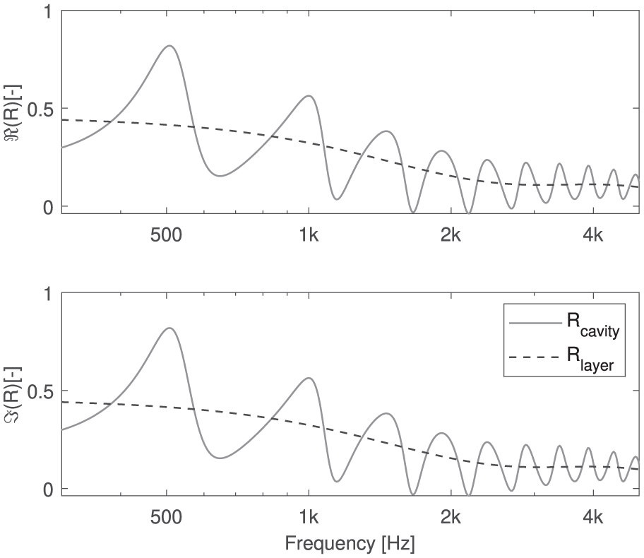
Predictions of normal–incidence plane wave reflection coefficients of a porous layer of resistivity 20 kPa⋅s/m2 and thickness 40 mm, backed by a 300 mm air cavity (gray line) and backed by an infinite layer of air (black line). These models of reflections coefficients are calculated based on equations (11) and (4), respectively.
In Section “Experimental validation and discussion,” it will be shown that the characterization results obtained by this standalone layer approach have greater accuracy than the results from the impedance model of a porous layer backed by an air cavity (the multilayer model, described in Section “Reference multilayer model”).
Another approach to deal with the problem could be to use a model of sound field that account for the fact that the wave front is spherical above the layer, such as the iterative “Q–term” or “F–term” algorithms. 17 However, this approach greatly increases the mathematical complexity and computational costs of retrieving the parameters. The method presented here provides an alternative to a more computationally expensive approach to characterized porous layers backed by a large air cavity.
Impulse response measurements
The acoustic pressure and normal particle velocity impulse responses (IRs) are recorded using a PU probe positioned close to the surface of the material (h < 20 mm) which is exposed to a normally incident sound wave, as well as in free field, using a small sound source located directly above the probe at a distance of d = 260 mm. The short probe-to-material surface
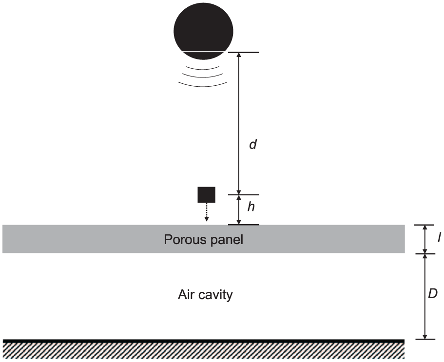
Arrangement of the sound source and PU probe above a porous layer backed by an air cavity to measure
Similarly to the case of the hard–backed layer of the previous publication,13 a time–windowing step with the Adrienne window
20
is used to remove the late parasitic reflections from the analyzed signal, before the impedances away from the material surface,
where
Estimation of the flow resistivity and thickness of the porous layer
The measured reflection coefficient is compared to the expected reflection coefficient of a standalone porous layer, based on the empirical Delany–Bazley–Miki (DBM) model.
22
The DBM model estimates the numerical values of the characteristic impedance,
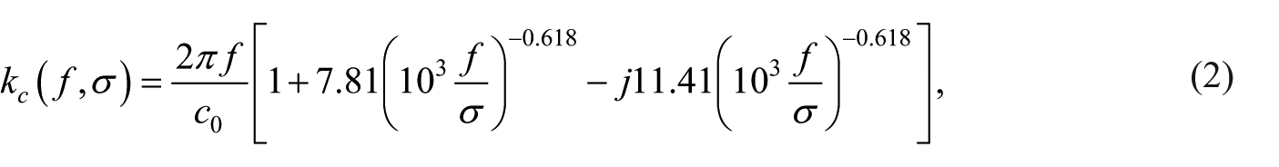
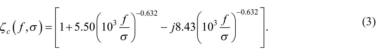
The frequency range of validity of the DBM is restricted to values of
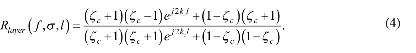
The plane wave reflection coefficient for a normal incident sound wave of the standalone porous layer of thickness
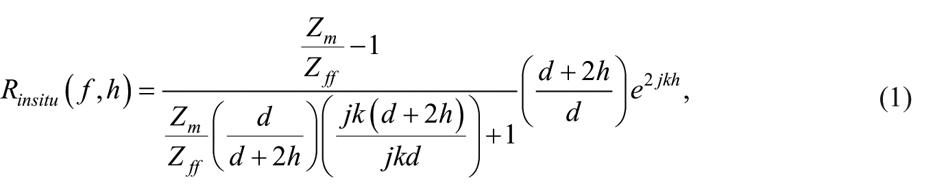
Utilizing equations (1) and (4), a cost function is set to minimize the difference between the measured reflection coefficient obtained from the measurements,
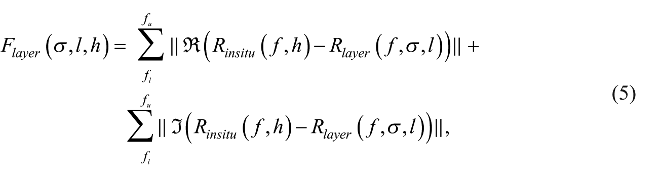
where
The model fitting frequency range in this work is
To obtain equal weights per octave bands, the frequency vectors used in Equation (5) were spaced logarithmically with 100 frequencies per band. The cost function,
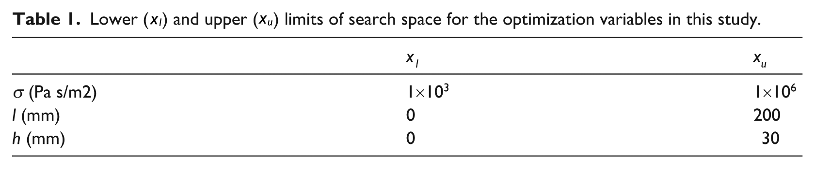
The search space, defined by the lower (
Lower (
The parameters yielding the best fitting (named hereinafter
Estimation of the air cavity depth
Following the completion of the model fitting, estimations of the thickness of the porous layer,
The air cavity depth is here estimated by analysis of the resonance peaks in the measured reflection coefficients, using the previously estimated porous layer thickness,
where
In the above equation,
As it is crucial that the peaks are prominent for peak detection, the detection was performed on the real part of the difference between the measured data (whose spectrum features the oscillations), and the fitted layer model (which does not feature the oscillations)
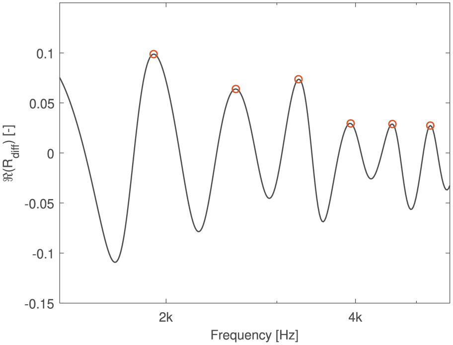
Illustration of a resonance peak detection on
Reference multilayer model
To investigate the benefit of this standalone layer approach for the in situ characterization of porous layers backed by large air cavities, an additional characterization was undertaken (only in the case for the experimental validation) using a direct model fitting of the measured data with the multilayer model of a porous layer backed by an air cavity. In this approach, the cost function is modified to
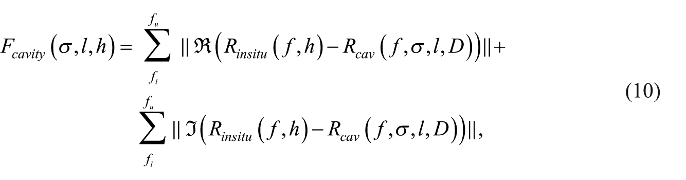
where
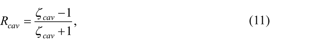
with
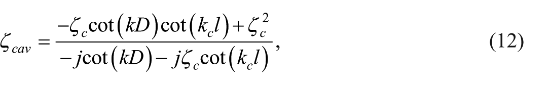
where
Numerical validation
Validation method
The accuracy of the proposed characterization procedure was tested through numerical simulations. This was done in a 2D setting to allow faster calculation time. The numerical method the in–house discontinuous Galerkin (DG) 2D solver for the wave equation, 25 with which the conditions of the in situ measurements were mimicked.
The impulse responses of the simulated acoustic pressure and particle velocity were captured at a distance hsim = 10mm above the surface of a 2D panel of very large dimension ( Lsim = 5m). This large dimension was chosen to avoid any size effect, which could otherwise induce measurement errors because of interferences with diffracted sound waves on the edges of the material.
26
The loudspeaker was simulated as an initial Gaussian distribution of acoustic pressure (Gaussian pulse) distributed around the source location with half–width w = 20mm, to reproduce frequencies up to 10 kHz, and vertically aligned with the receiver at a distance d = 260mm. Details on the implementation of the source can be found in the literature.
25
The simulated measurement environment is a 5 × 5 m 2D room with perfectly hard boundaries (
The mesh of the 2D space (made of triangle elements) was implemented using the freeware GMSH
27
with a characteristic element length,
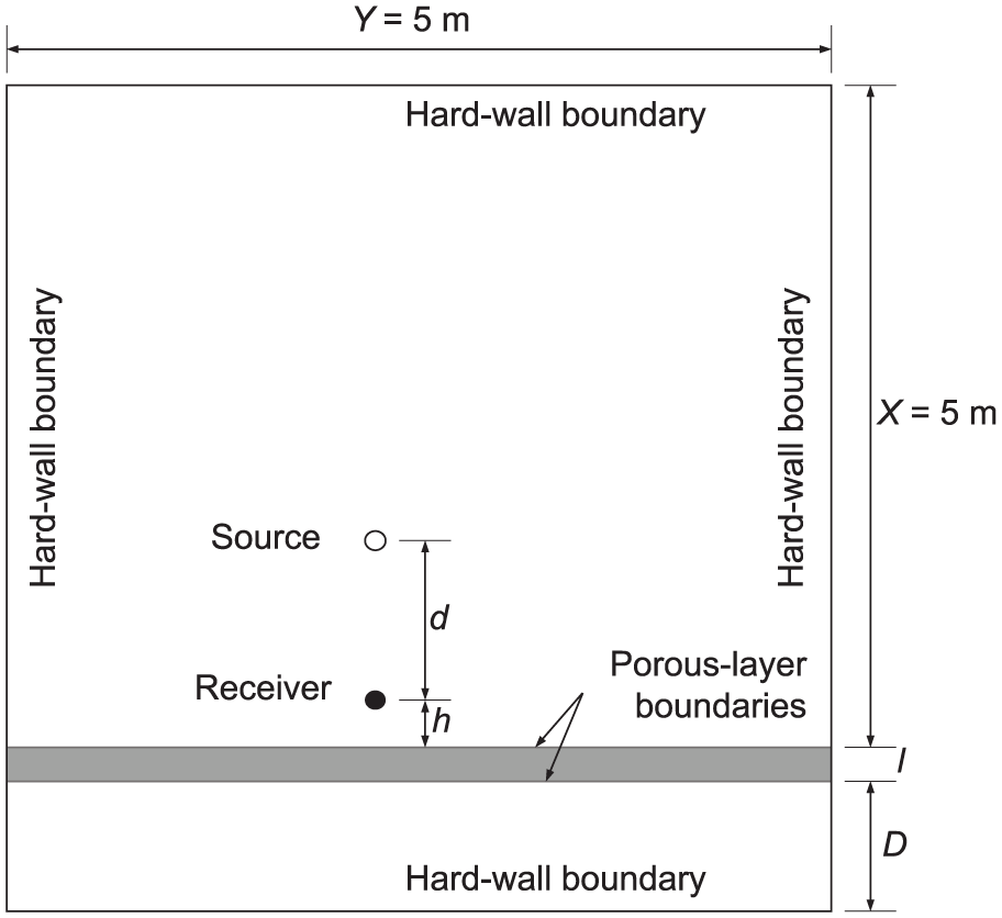
Geometry of the 2D simulation setup.
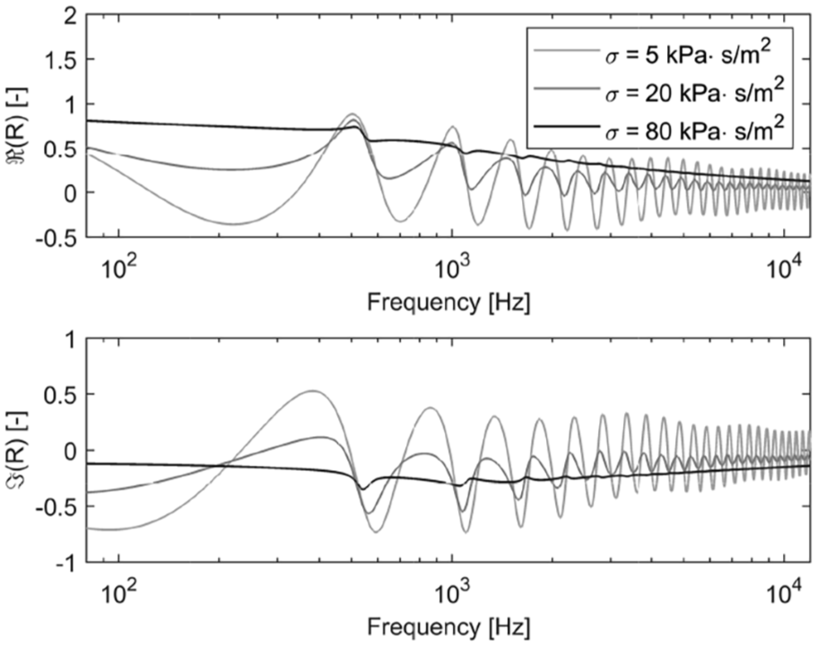
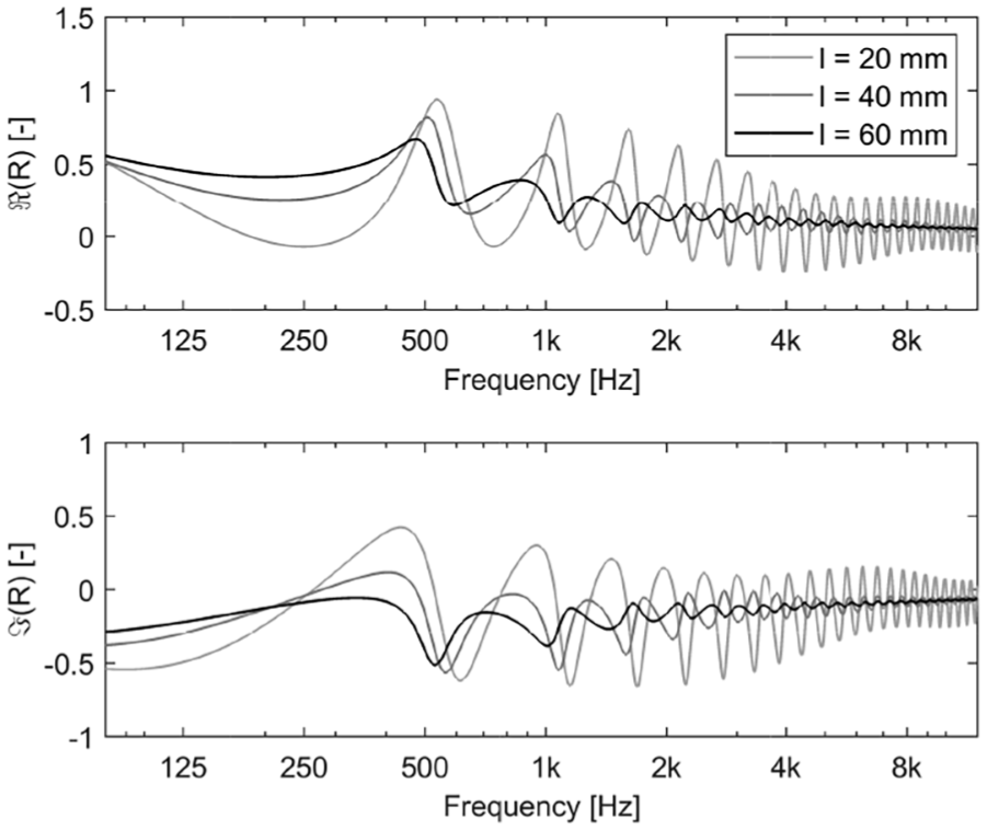
To verify that the accuracy of the method was not case–dependent, the procedure was tested numerically on 75 simulated cases of porous layers on rigidly backed air cavities (D ≥ 100 mm). The simulated flow resistivities of the porous layers ranged from 5.0 to 80.0 kPa⋅s/m2 in steps of doubled values (5, 10, 20, 40 and 80 kPa⋅s/m2), while the thicknesses were varied between 20, 40 and 60 mm. The cavity depth was varied in steps of 100 mm from 100 mm to 500 mm. Examples of how the various parameters theoretically influence the plane wave normal incidence reflection coefficient are shown in Figures 5–7.
Theoretical reflection coefficient of systems with porous layer thickness l = 40 mm, cavity depth
Theoretical reflection coefficient of systems with porous layer resistivity σ = 20 kPa⋅s/m2, cavity depth
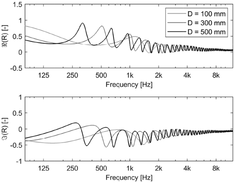
Theoretical reflection coefficient of systems with porous layer resistivity σ = 20 kPa⋅s/m2, thickness l = 40 mm and varying cavity depth.
Numerical validation results
The results of the characterization procedure performed on the simulated systems are presented in Tables 2–6, which display the results for the porous layer of flow resistivities of the porous layer of 80, 40, 20, 10 and 5 kPa⋅s/m2, respectively. Within these tables, the cells where the error in the retrieved parameter is above 10% are colored in light gray, while the ones with an error above 15% are colored in dark gray.
Characterization results of simulated systems with σ = 80kPa⋅s/m2. The optimal values
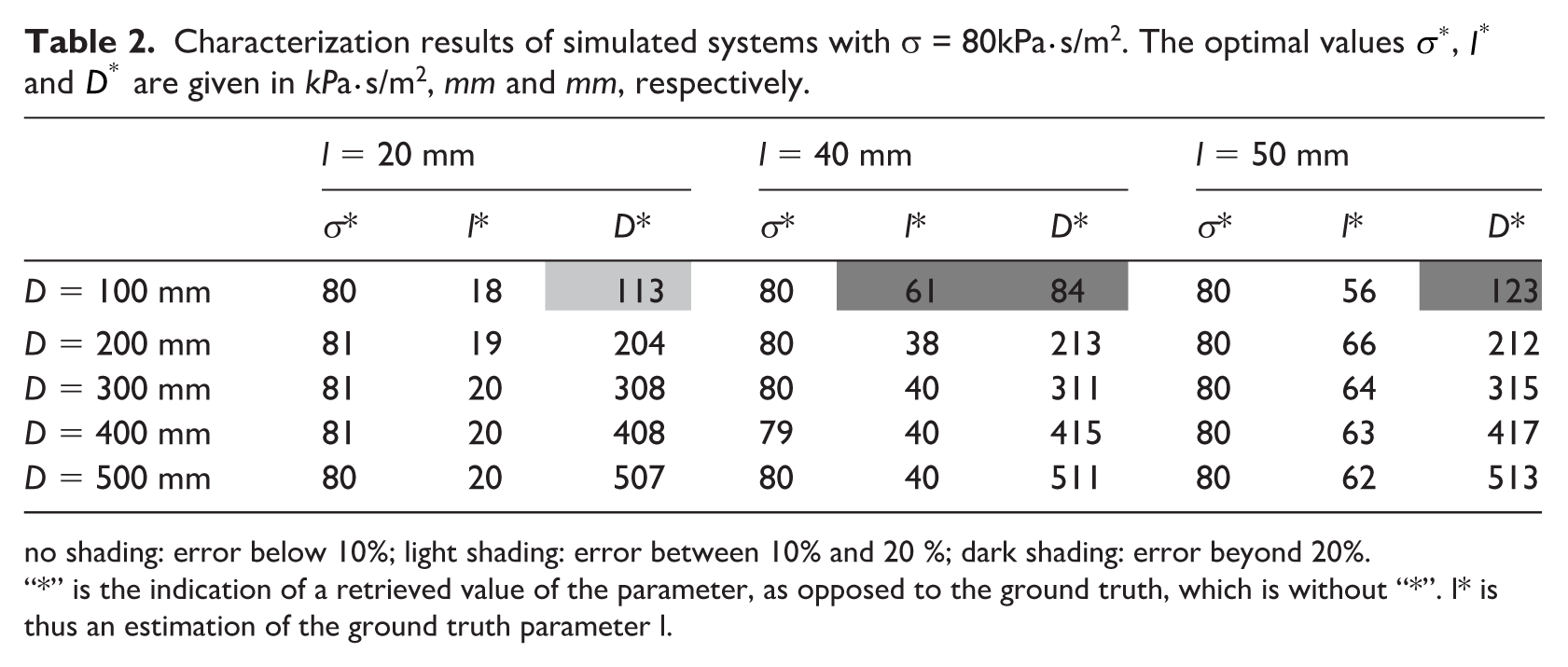
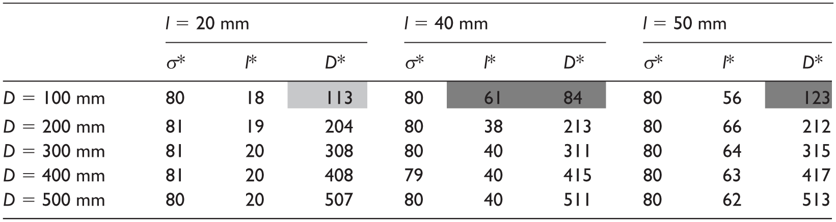
no shading: error below 10%; light shading: error between 10% and 20 %; dark shading: error beyond 20%.
“*” is the indication of a retrieved value of the parameter, as opposed to the ground truth, which is without “*”. l* is thus an estimation of the ground truth parameter l.
Characterization results of simulated systems with σ = 40 kPa⋅s/m2. The optimal values
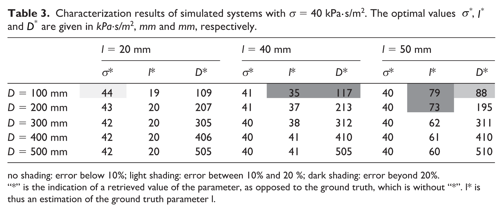
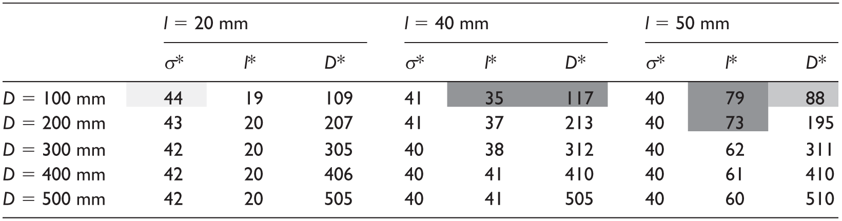
no shading: error below 10%; light shading: error between 10% and 20 %; dark shading: error beyond 20%.
“*” is the indication of a retrieved value of the parameter, as opposed to the ground truth, which is without “*”. l* is thus an estimation of the ground truth parameter l.
Characterization results of simulated systems with σ = 20 kPa⋅s/m2. The optimal values
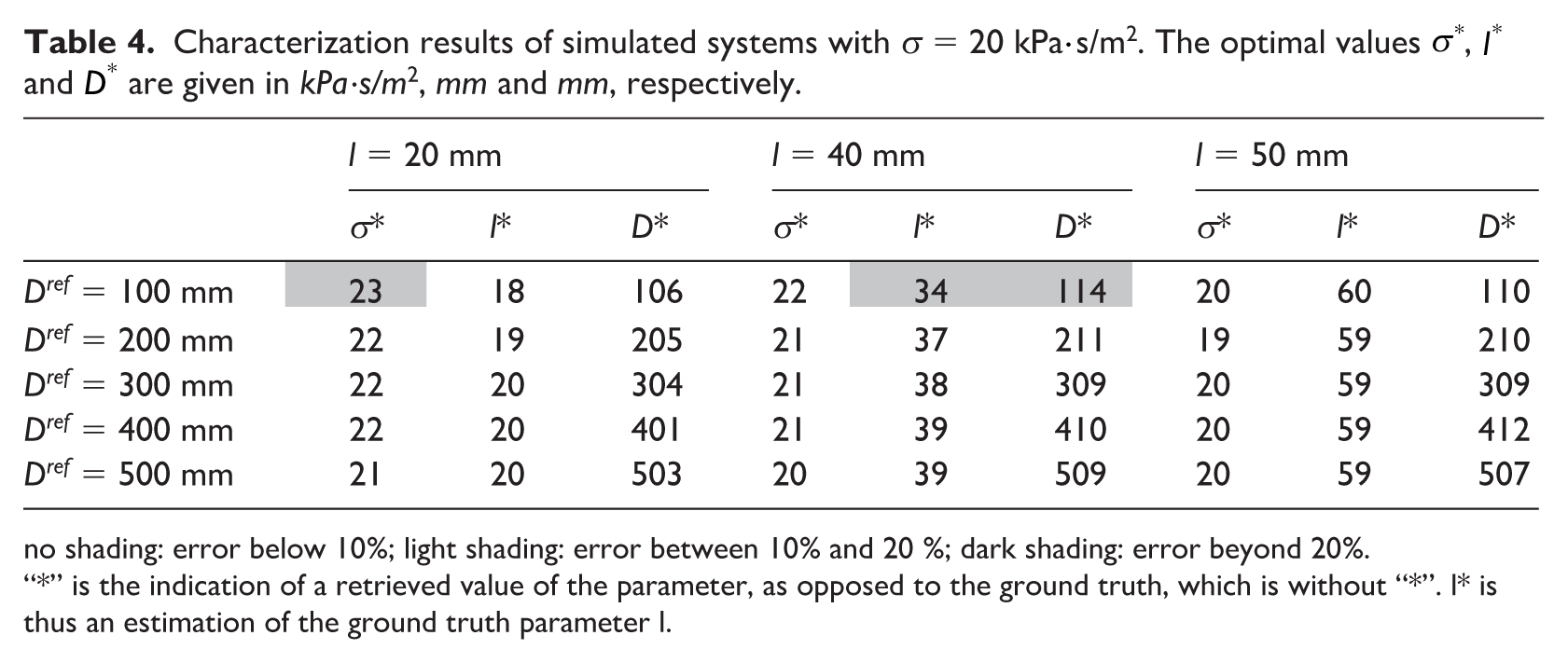
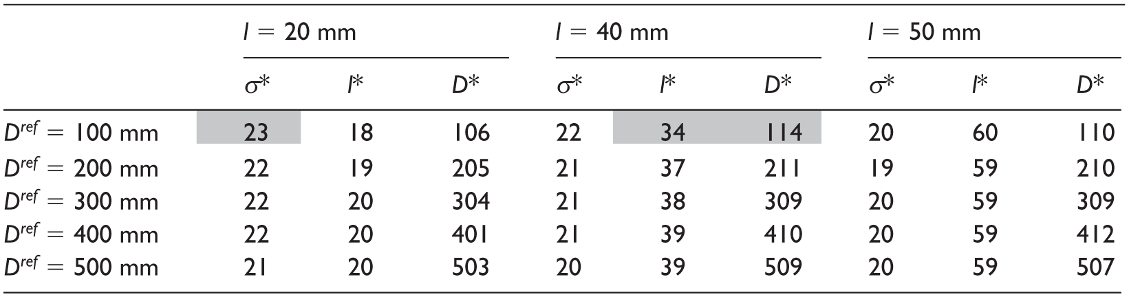
no shading: error below 10%; light shading: error between 10% and 20 %; dark shading: error beyond 20%.
“*” is the indication of a retrieved value of the parameter, as opposed to the ground truth, which is without “*”. l* is thus an estimation of the ground truth parameter l.
Characterization results of simulated systems with σ = 10 kPa⋅s/m2. The optimal values
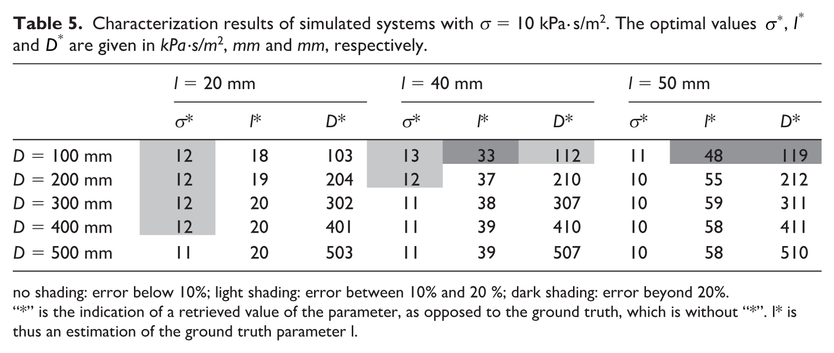
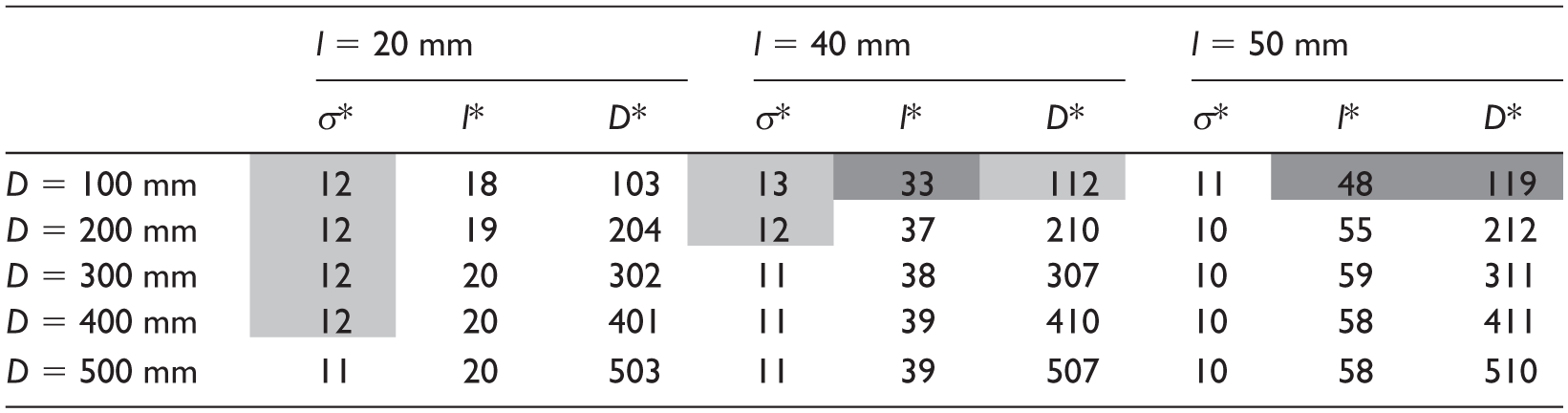
no shading: error below 10%; light shading: error between 10% and 20 %; dark shading: error beyond 20%.
“*” is the indication of a retrieved value of the parameter, as opposed to the ground truth, which is without “*”. l* is thus an estimation of the ground truth parameter l.
Characterization results of simulated systems with σ = 5.0 kPa⋅s/m2. The optimal values
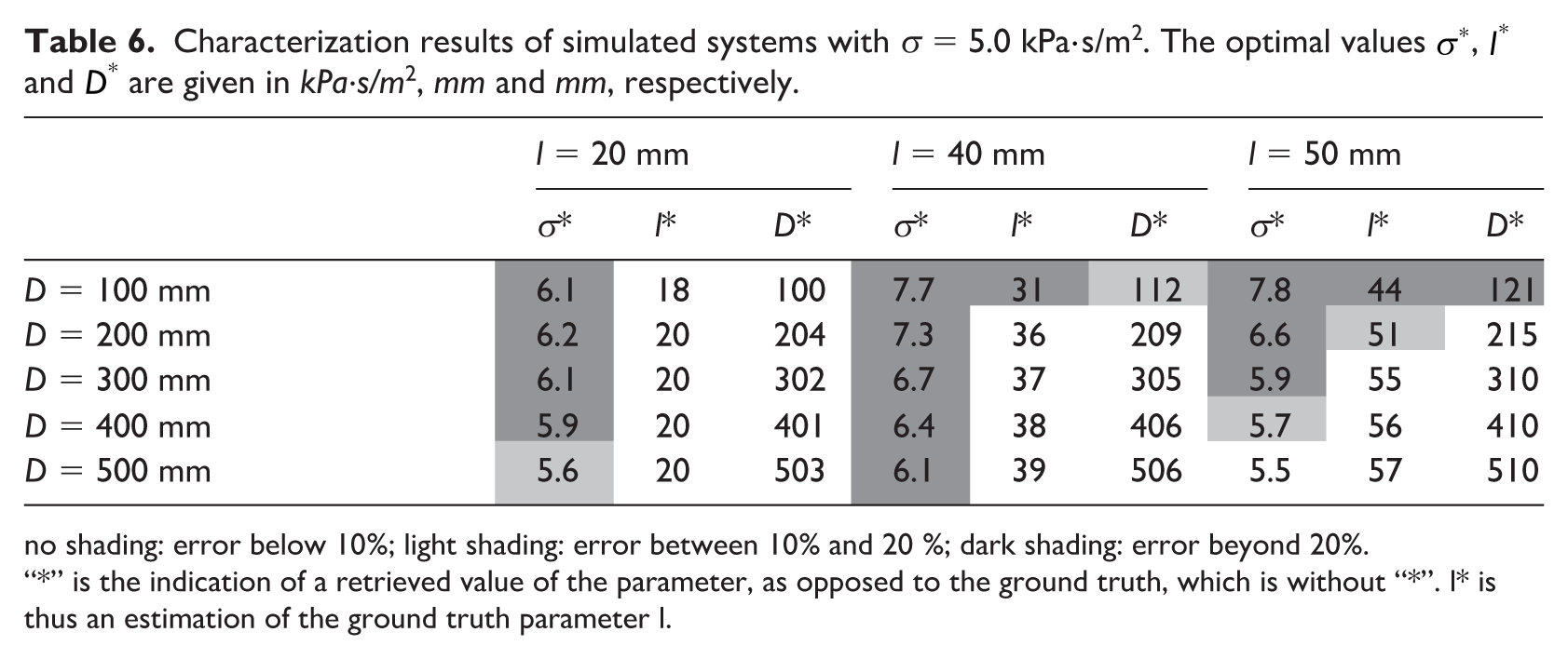
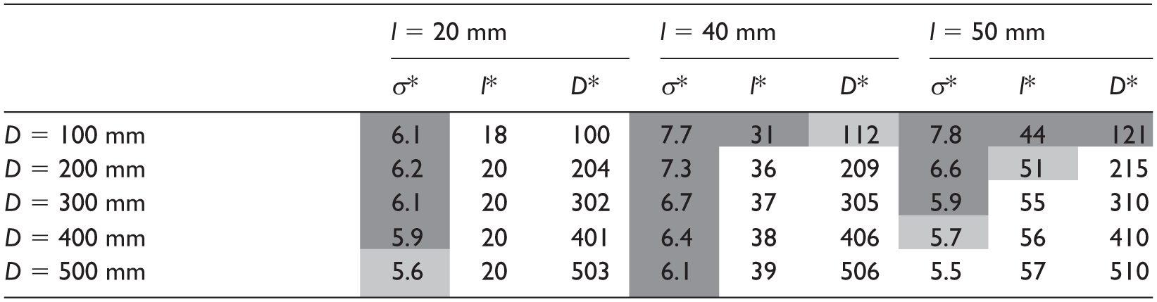
no shading: error below 10%; light shading: error between 10% and 20 %; dark shading: error beyond 20%.
“*” is the indication of a retrieved value of the parameter, as opposed to the ground truth, which is without “*”. l* is thus an estimation of the ground truth parameter l.
The results for a porous layer with a flow resistivity of 80 kPa⋅s/m2 (Table 2) show that for nearly all combinations of thickness and cavity depth tested, the error in retrieved flow resistivity is smaller than 10%. The error in retrieved thicknesses and cavity depths, however, increases significantly for the smaller air cavity depth tested (100 mm). This can be explained by the fact that, as distance to the reflective wall at the end of the air cavity increase, the system’s behavior more closely approximates that of a standalone porous layer. Conversely, when the cavity depth reduces, the system behaves less like a standalone porous layer. For cavity depths of 200 mm or more, the relative error for these two parameters is equal to or below 10%.
Similar observations can be made for the cases where the porous layer has a flow resistivity of 40 kPa⋅s/m and 20 kPa⋅s/m2 (Tables 3 and 4). The error in retrieved flow resistivity, thickness and cavity depth remains small for all the configurations simulated, but the errors in thickness and cavity depth are more significant for the systems with a cavity depth of 100 mm. However, an exception is observed for the system with a porous layer of 60 mm thickness and flow resistivity of 40 kPa⋅s/m2 (Table 3), where a large error in retrieved thickness is observed for an air cavity of 200 mm. This is likely because for this particular system, the reflection coefficient varies only very little with changes in thickness, especially for the frequency range above 1 kHz. This can be observed when comparing the predictions of the plane wave normal incidence reflection coefficient computed using the reference parameters and the retrieved parameters, shown in Figure 8.
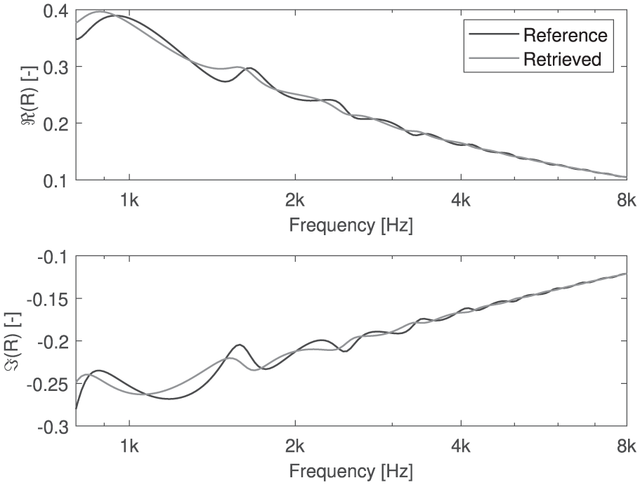
Comparison of the plane wave normal reflection coefficient as computed from the reference values and the retrieved values for the case of a porous layer of resistivity σ = 10 kPa⋅s/m2 and thickness l = 40 mm backed by an air cavity D = 200 mm.
For the simulated systems with the lowest flow resistivities (10 kPa⋅s/m2 and 5 kPa⋅s/m2,Tables 5 and 6), the relative error in retrieved resistivity also becomes larger for the systems with larger cavities, but that is mostly because the true resistivity is much lower. However, the absolute error value remains below 3 kPa⋅s/m2, which is obtained for the systems of lowest flow resistivity with the shallower air cavities.
Overall, the numerical study suggests that the proposed method to characterize a porous layer with a large backing cavity provides low error in retrieved parameters for a wide range of layer/cavity depth combinations, as long as the cavity depth is sufficiently large (D ≥ 200 mm).
Experimental validation and discussion
Measurement setup
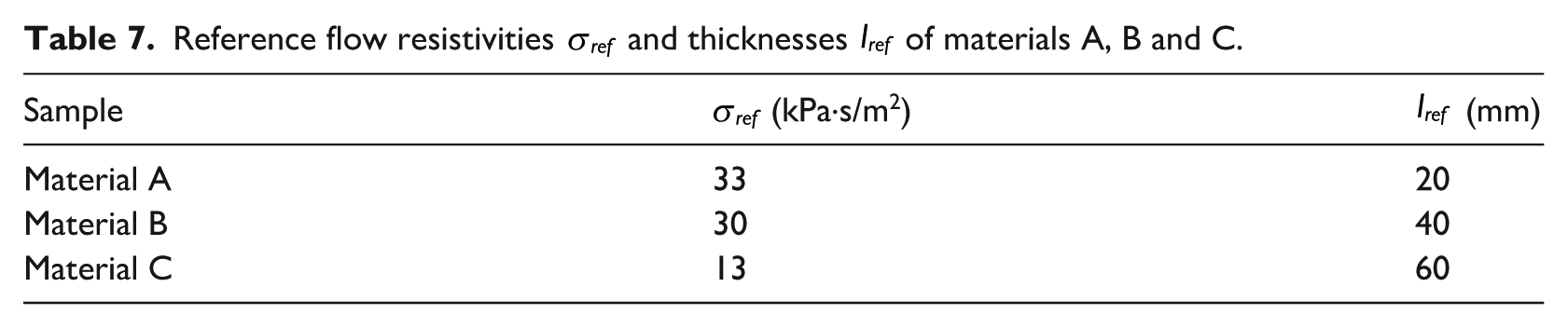
Following the results obtained from the numerical study, the experimental validation of the procedure was performed on three porous layers (materials A, B and C) with three cavity depths: 160 mm, 240 mm and 500 mm, that were mounted above a concrete floor. The dimensions of the samples were 500 × 500 mm for Materials A and B, and 600 × 1000 mm for Material C. These lateral dimensions, which exceed 1.4 times the longest wavelength measured, were considered sufficient to avoid significant size effects within the range 1–8 kHz, which is the frequency range measured. The reference flow resistivities and thicknesses of the three samples are shown in Table 7. The flow resistivities were obtained from the low–frequency limit of the imaginary part of the dynamic mass density, 29 extracted from impedance tube measurements via the two-cavity method. 30 The flow resistivities extracted suggests that the modeling of the materials with the DBM is valid at least in the range (650–13,000) Hz, which encompasses the range of interest.
Reference flow resistivities
The measurements were made using the “In Situ Absorption Testing” measurement hardware (manufactured by Microflown Technologies). It consists of a PU probe attached to a small round loudspeaker via a light decoupling structure, which sets the source–to–probe distance to 260 mm. The device can be seen in the measurement configuration in Figure 9. The source signal, a 5–second exponential sweep sine, was produced from a laptop running the room acoustic software DIRAC 6 room acoustics acquisition software (Acoustics Engineering). The signal was sent to an amplifier before being sent to the source. The acquired signals were recorded by the same laptop and the de–convolutions into impulse responses were performed by DIRAC 6.
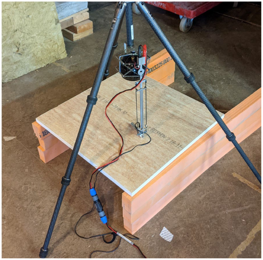
The experimental validation setup. The sample of material B is mounted on rubber bars to create a 240 mm air gap between the sample and the concrete. It can be seen that a label is printed on the surface of the materials, the influence of this print was neglected.
The setup was positioned close to the panel’s surface with the help of a tripod so that the probe was located at a height href = 10 mm above the surface and the source vertically aligned with the probe, as shown in Figure 9, and oriented so that the direct sound reached the sample with normal incidence. The velocity sensor was carefully oriented to capture the velocity component orthogonal to the sample’s surface. As for the horizontal location above the plane, the PU probe was placed within the confidence region for PU probe measurements, to limit the influence of the sound waves diffracted by the edges of the samples.
17
Thus, the probe was placed within a distance of
The measurements were conducted in the workshop space of the Echo building at Eindhoven University of Technology, which features a 300mm–thick concrete floor used as the hard wall at the bottom of the air cavities. The porous layers were held above the floor with rubber beams stacked together to achieve the intended cavity depths. The workshop contained various equipment and measurement installations, but an area of about a 1.5 m radius around the measurement location was cleared to avoid strong parasitic reflections from neighboring objects. With such a clearance radius, the time windowing of the impulse responses was chosen to include the reflection from the concrete floor in the largest air gap configuration (500 mm), while windowing out the later reflections from the neighboring environment. These considerations led to the use of an Adrienne window with a total time length of 8 ms for the time–windowing of the impulse responses. The main drawback of this short windowing is that the low frequency information (mostly below 500 Hz) is increasingly distorted. The impact of this fact on the method is however limited since only higher frequencies are analyzed.
Results
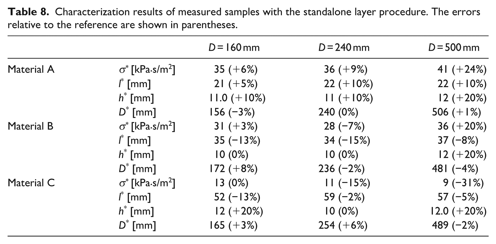
The characterization results of the experiment are given in Table 8, and an example of the obtained fitting is shown in Figure 10. For each configuration measured, the optimal parameters
Characterization results of measured samples with the standalone layer procedure. The errors relative to the reference are shown in parentheses.
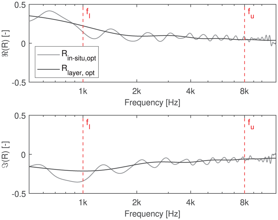
Comparison of measured reflection coefficient (Material C with a 160 mm cavity) and fitted model of standalone layer. A similar global trend within the fitting frequency range (delimited with red lines) is observed between the case with the air cavity, which is measured (
The values retrieved for the flow resistivity vary significantly depending on the air cavity depth behind the sample, with the error to the reference value being greater for a larger air cavity. This is an unexpected result, as this error trend was not visible in the numerical results in Section “Numerical validation.” The reason for this could be that the side walls used to create the cavity (which are not accounted for in the model) redirect a significant amount of sound energy toward the layer, in turn increasing the sound energy reflected from the layer’s surface compared to a cavity without walls and therefore affecting the model of porous material fit to the measured coefficient.
The retrieved thickness values are, however, in good agreement with the references, with a maximum observed deviation of 15% (Material B with 240 mm cavity). The retrieved cavity depths are also in very good agreement with the reference, with deviations less than 8%. In absolute terms, the deviations observed correspond to, at most, a 6 mm error for the porous layer thickness and a 19 mm error for the cavity depth. Also, the retrieved values for the probe–to–sample distance are always within 3 mm deviation of the measured distance (10 mm), which suggests that using
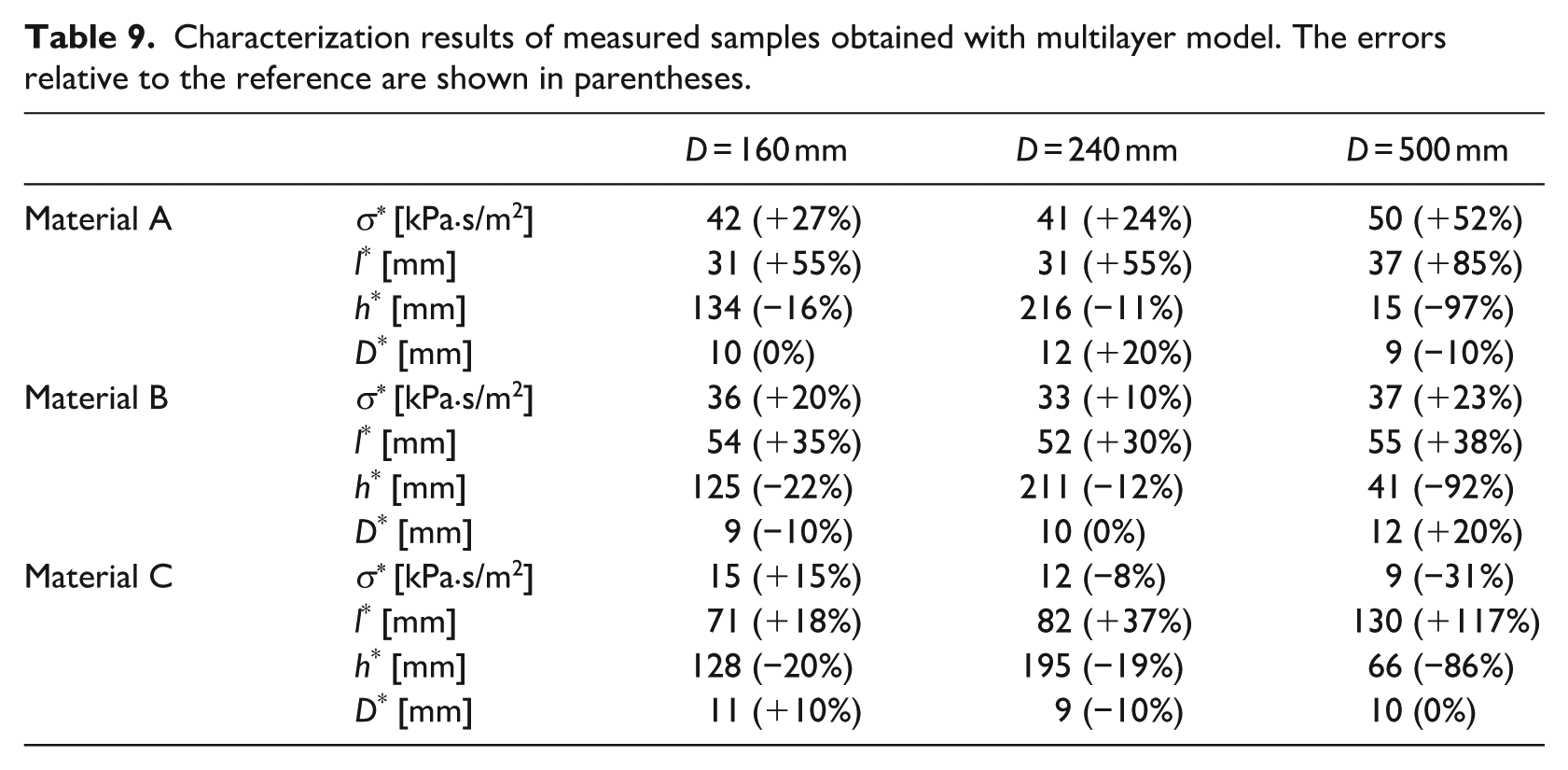
The results presented in Table 8 should be compared with the results obtained using the multilayer model of a porous layer backed by an air cavity (presented in Section “Reference multilayer model”), presented in Table 9. The errors are much greater when using the regular model, as expected. The error is above 15% for nearly every parameter in every configuration, except for Material C, for which the flow resistivity is still retrieved with good accuracy. The errors are largest in the case of the largest air cavity (500 mm).
Characterization results of measured samples obtained with multilayer model. The errors relative to the reference are shown in parentheses.
To investigate the influence of the characterization error on the modeling of the acoustic properties, the plane wave normal incidence absorption coefficient was computed in 1/3–octave bands from the retrieved parameters
with
where
The results are shown in Figures 11–13 for Materials A, B and C, respectively, in the frequency range 80–12 kHz. The root mean square (RMS) errors for each case are reported in Table 10.
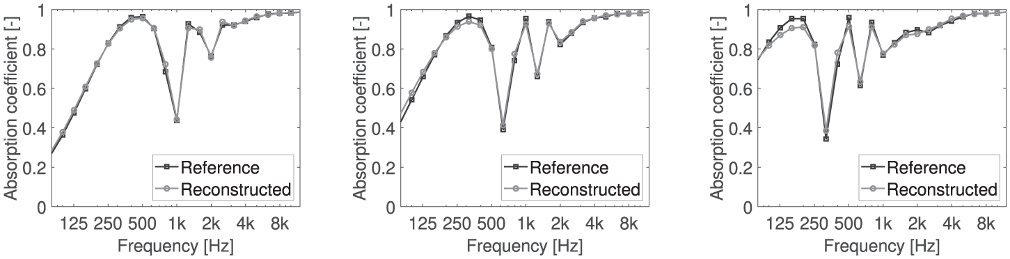
Reference and reconstructed absorption coefficients of the porous layer backed by an air cavity (normal incidence) featuring Material A with different cavity depths. Left: 160 mm, center: 240 mm, right: 500 mm.
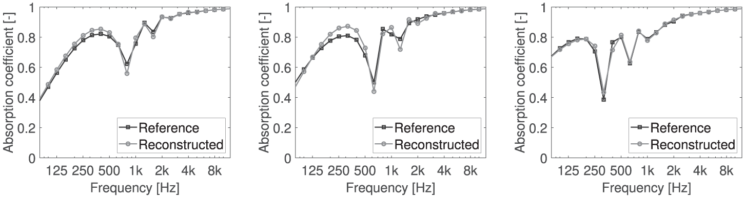
Reference and reconstructed absorption coefficients of the porous layer backed by an air cavity (normal incidence) featuring Material B with different cavity depths. Left: 160 mm, center: 240 mm, right: 500 mm.
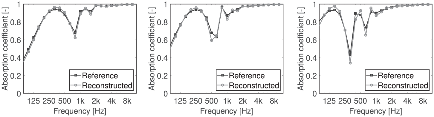
Reference and reconstructed absorption coefficients of the porous layer backed by an air cavity (normal incidence) featuring Material C with different cavity depths. Left: 160 mm, center: 240 mm, right: 500 mm.
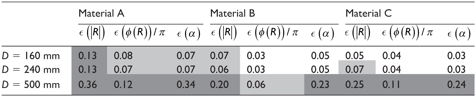
Root mean square (RMS) error of the reconstructed acoustic properties to the reference, computed from 1/3–octave band averages from 100 Hz to 10 kHz using the proposed method (standalone layer model). Cells showing RMS errors above 0.05 are highlighted in light gray.
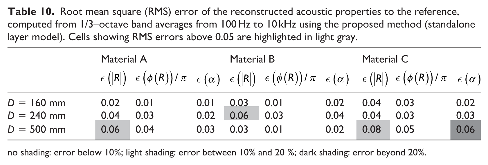
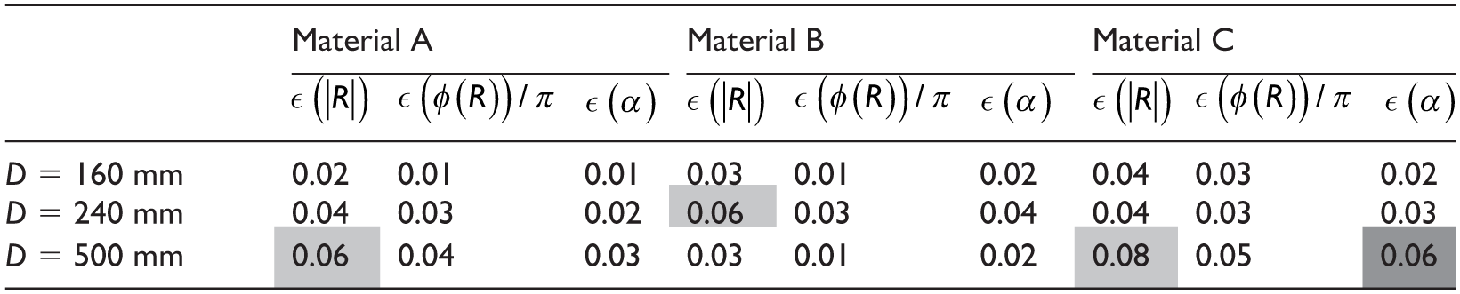
no shading: error below 10%; light shading: error between 10% and 20 %; dark shading: error beyond 20%.
The figures show that the reconstructed absorption coefficients are in good agreement with the references for all the measured systems, particularly above 500 Hz. In most of the measured cases, the error in 1/3–octave bands appears negligible. However, for some cases, such as Material B with a 240 mm cavity (Figure 12, center) and Material C with a 500 mm cavity (Figure 13, right) visible errors are observed in the 1/3–octave bands below 500 Hz. These errors are most likely resulting from the non-accuracy of the plane wave assumption at these frequencies, because of the relatively short source-to-probe distance and lateral dimensions of the sample used, which are becoming comparable or shorter than the wavelengths. A potential solution to decrease these discrepancies would then be to increase the sample size and source-to-probe distance. This could however reduce the signal-to-noise ratio in in-situ conditions, and in practice a balance would have to be found.
It should be noted that regarding the ’reconstructed’ reflection coefficients, the points above 1 kHz are based on a fitting of the reflection model to the data actually measured. On the other hand, below 1 kHz, the absorption profile is only extrapolated from the fitted model. Higher discrepancies were therefore expected below 1 kHz.
From Table 10, the RMS errors observed in the absorption coefficient reach a maximum of 0.08, obtained for Material C backed with a 500 mm–thick cavity and correspond to a case where the amplitudes of resonance are very pronounced. For all the other cases, the maximum error remains below 0.06 (or
These values should be compared with the results obtained from the use of the multilayer model in Table 11. A comparison of the two tables shows that, compared to the multilayer model approach, the standalone layer method provides more accurate results in terms of acoustic property reconstruction in all cases. This accuracy advantage is the greatest for systems with a 500 mm cavity depth. The comparison also shows that the standalone porous layer method is more advantageous for systems featuring a thin porous layer (Material A).
Root mean square (RMS) error of the reconstructed acoustic properties to the reference, computed from 1/3–octave band averages from 100 Hz to 10 kHz using the reference model (multilayer model). Cells showing RMS errors above 0.05 are highlighted in light gray and the ones showing errors above 0.08 in dark gray.
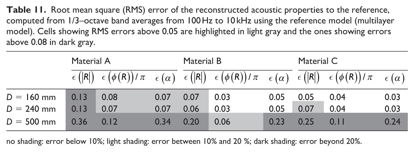
no shading: error below 10%; light shading: error between 10% and 20 %; dark shading: error beyond 20%.
These results demonstrate that the in situ characterization procedure provides a prediction of the acoustic absorption of the system that is in good agreement with the prediction obtained from the reference parameters. Furthermore, comparison with the results obtained from the multilayer model shows that the proposed method performs a better in reconstruction of acoustic properties, particularly in the case of a very large cavity and/or a thin porous layer.
Conclusions
This study presents a technique for in situ characterization of a porous panel backed by a large air cavity. The approach presented involves a PU probe measurement, a model fitting process and a resonance analysis.
The originality of the model fitting process is that the measured data is fitted with the model of a standalone porous layer in a limited frequency range. This process avoids the impact of the air cavity and allows the retrieval of the flow resistivity and the thickness of the layer. Following the retrieval of the porous layer’s parameters, analysis of the frequencies in the reflection coefficient resonance peaks allows an estimation of the depth of the hard–backed air cavity.
To support the proposed method, the accuracy of the procedure was first evaluated through a simulation study of 75 individual systems of porous layers backed by air cavities, covering a wide range of porous layers used in room acoustics and cavity depths found in suspended ceiling systems. The results of this simulation study showed the validity of the method for systems of porous layers backed by large air cavities, with errors in retrieved parameters below 10% when the air cavity of the system was 200 mm or higher. Larger relative errors were obtained for the retrieved resistivity of the layer when the reference resistivity was low, but the absolute deviation remained small.
The procedure was then tested experimentally with the characterization of nine combinations of porous layers backed by air cavities. The analysis of the experimental results revealed that the method yields accurate estimations of the porous layer flow resistivities, thickness, and cavity depth, with a maximum error of 15% in retrieved parameters when the cavity depth was of 160 mm or 240 mm. Greater deviations, up to 24%, were observed for a cavity depth of 500 mm, but remained in all cases smaller that the errors observed when using a standard multilayer approach to characterize the system.
Although deviations were observed in the obtained parameters with the presented approach, the error associated with the predicted absorption coefficient, calculated in 1/3-octave band averages for normal plane wave incidence, was minimal when compared to the reference results. The maximum root mean square (RMS) deviation observed was 0.08, all significant error being found in the 500 Hz octave band and below. This result suggests that the proposed method for characterizing suspended ceiling systems leads to an accurate estimation of the acoustic properties, especially in the high–frequency region.
Future works of interests include testing the applicability of this method to different nature of materials, and in particular the ones whose properties are rules by different models. The integration of a coating layer into the model fitting is another element of great interest, as many commercial sample feature such an impermeable coating.
Footnotes
Appendix
Declaration of conflicting interests
The authors declared no potential conflicts of interest with respect to the research, authorship, and/or publication of this article.
Funding
The authors disclosed receipt of the following financial support for the research, authorship, and/or publication of this article: This project has received funding from the European Union’s Horizon 2020 research and innovation programme under the Marie Sklodowska-Curie grant agreement number 721536.