
Abstract
Due to inherent nonlinear stiffness and damping characteristics, dry friction interfaces have a significant impact on the dynamics of jointed structures. When two surfaces are brought into purely normal contact, contact pressure distribution is of high concern. This work focused on the statistics of the contact pressure distribution between a rough surface and a smooth rigid plane, which provides new insight into the interface contact behaviour. First, the fractal rough surface is generated using the Weierstrass–Mandelbrot function with measured roughness parameters. With meshed rough surfaces, an elastic–plastic finite element contact analysis is performed to determine the contact pressure distribution. Then, the results of contact pressure are statistically analysed. The effects of roughness and contact load on contact area, contact stiffness and mean contact pressure are thoroughly investigated. The probability distribution of contact pressure is determined by fitting a continuous function using a twofold Weibull mixture model. The proposed probability distribution function is found to be capable of describing contact pressure. The contact pressure distribution is affected by the surface fractal characteristics and evolves with the contact load.
Introduction
Dry frictional joints, such as bolted joints and riveted joints, are widely applied in mechanical and aerospace engineering. 1 Subjected to vibration excitation, contact and slip between frictional surfaces result in the nonlinear dynamic response of the jointed structure. It is very important to understand the interface contact and friction characteristics for accurately predicting the dynamics of structures with frictional joints.
The most recent investigations have revealed that the nonlinear dynamic response is highly sensitive to the contact pressure distribution pattern at the contact interface of the friction joint.2–7 Schwingshackl et al. 4 divided the frictional interface of an under-platform damper (UPD) into five regions with uniform pressure distribution and assigned five different constant pressure values at each region. Although the contact pressure distributions in their studies were randomly generated and do not represent real contact status, the results emphasized the effect of contact pressure distributions on vibration amplitude. Following this, Schwingshackl et al. 5 conducted a close visual inspection of a flange joint and identified that a slightly convex shape presented in the interfaces was due to manufacturing imperfections. Thus, they modified the pressure value of individual nodes located along the top and bottom edges of the interface to get a more realistic contact pressure distribution. The modified contact pressure distribution shows higher accuracy in predicting damping than that of not considering manufacturing imperfections. Furthermore, an analytical pressure distribution, which is the sum of two exponentials (one with a positive exponent and the other with a negative exponent), is proposed to describe the concave shape and convex shape of the frictional interface due to manufacturing imperfections. 6
These investigations highlight the effect of contact pressure distribution patterns on the mechanical response of jointed structures. However, these works only explore the contact pressure distribution resulting from macroscale shape deviation or mesoscale waviness. It is well-known that the real contact surface is covered with microscopic asperities. Therefore, it is vital to explore the real contact pressure distribution caused by these microscale rough characteristics.
Contact pressure distribution due to the macroscopic interface can be easily measured using the pressure-sensitive film. 8 However, the lateral resolution of the pressure-sensitive film is restricted by the size of the ink microcapsules. Thus, the local distribution of the contact pressure due to the microscopic feature of the contact interface can hardly be observed. The optical method9,10 is an alternative approach for in-situ measurement of the contact pressure distribution. One type of these methods relies on pre-calibration to accurately set up the correlation between the light intensity and the contact pressure. The other methods measure the three-dimensional (3D) displacement field and then the contact pressure distribution is inversely calculated based on the Boussinesq solutions. Due to the requirement that one of the contact bodies should be transparent, the optical approach is not feasible for mechanical joints.
There are many investigations on elastoplastic rough surface contact11,12 and loading–unloading contact between rough surfaces.13–15 However, only Persson's theory can directly predict the probability density function (PDF) of the contact pressure distribution.16,17 The constant hardness assumption is adopted to approximate the elastic-perfectly-plastic material model. This assumption states that the contact pressure cannot exceed
The finite element (FE) method and boundary element method are two numerical approaches for solving rough surface elastoplastic contact. Boundary element method20–22 is less popular since the development of the elastoplastic contact model is less straightforward than its linear elastic counterpart, especially when a more realistic J2 plasticity model is implemented. Therefore, the FE method has mainly been regarded as the dominant approach for analysing the contact behaviour of rough surfaces.
The first step of FE rough contact analysis is to generate the rough surface data for establishing the FE model. Generally, there are mainly two kinds of methods applied to obtain the rough surface data for the FE simulation. One is collecting the measured surface data directly, and the other is utilizing geometry description. Thompson et al.23,24 used the white light interferometer to measure surface data for generating rough surface and found that it is important to consider the sub-surface mesh density for obtaining convergence and reliable results in a rough FE model. On the other hand, the multiscale fractal nature of rough surfaces has long been observed. 25
One of the dominant approaches is to generate the fractal rough surfaces using the Weierstrass–Mandelbrot (WM) function. 26 Sahoo et al.27,28 generated rough surfaces using a modified two-dimensional WM function and performed the FE analysis of an elastic–plastic contact with a rigid flat. Then parametric studies, including the effect of variation of fractal parameters on contact behaviour involving contact area, load and displacement, were conducted to describe the general relations between contact properties and surface parameters. Hyun et al. 29 generated fractal rough surfaces with a range of roughness amplitudes and roughness exponents using the successive random midpoint algorithm, which was also used by Pei et al. 30 to conduct the FE analysis of elastic–plastic contact between rough surfaces. Wang et al. 31 proposed a spectral interpolation method to construct rough surfaces in conjunction with the measured points and systematically studied elastic–plastic friction contact between rough surfaces and a rigid flat under the combined normal and tangential loading. The results of this study showed that the reduced real contact area due to roughness also governed the friction between the surfaces.
In summary, surface roughness is recognized as having a significant effect on contact friction behaviours and with the aid of FE simulation the contact behaviour, such as the relationship among normal load, normal displacement and real contact area are well investigated. However, the works studying the contact pressure distribution of rough surfaces with microscale asperities, which have an important influence on the nonlinear friction and dynamic response of the assembled structures, are still not sufficient. At present, there is no explicit method to describe the PDF of contact pressure. It is also noted that for interface nonlinear tangential friction modelling, several popular tangential models such as the original Iwan model,32,33 the four-parameter Iwan model, 34 the six-parameter Iwan model35,36 and so on, are derived by artificially predefining a probability density function (PDF) of critical slipping force or local normal contact pressure. Thus, this article focuses on establishing a mathematical description model with continuous function to determine the form of PDF explicitly.
To address these issues, the FE method is used to simulate the contact characteristics between a rough surface and a rigid plane, and the fractal method is used to describe the geometry of the rough surface. Considering the statistical characteristics and the microcontact mechanism of rough surfaces, the contact pressure distribution is analysed from a new statistical point of view to provide insight into contact pressure distribution and its mathematical description.
The article is organized as follows. In the ‘FE simulation methods’ section, a fractal rough surface is generated using the WM function with measured roughness parameters and the FE modelling method is introduced. In the ‘Simulation cases’ section, three FE models with different roughness are established. In the ‘Results and discussion’ section, the effects of roughness and the normal load on the contact area, contact stiffness and mean contact pressure are investigated. The probability density distribution of contact pressure is determined by mathematical statistics, and the effect of the roughness on the contact pressure distribution is discussed. In the ‘Conclusions’ section, the main conclusions are presented.
FE simulation methods
Fractal description of rough surface
It is well-known that all engineering surfaces are not perfectly smooth and different surface topography characteristics have a significant impact on the contact friction behaviour of connection surfaces and the dynamic response of assembled structures. In order to effectively predict the normal contact and tangential friction behaviour, it is important to accurately obtain the rough surface data. One of the dominant approaches to simulate the rough surface topography is based on the real surface microscopic geometric characteristics.
Microscopic observations have shown that engineering surfaces exhibit a self-affine structural property revealing similar geometrical features at various scales.37,38 Fractal geometry is characterized by continuity, non-differentiability, and self-affinity. These characteristics are considered to be related to the intrinsic physical laws that govern the generation of surfaces. 39 Thus, fractal theory can be used as an effective way to characterize multi-scale surface topography.
The WM function is an appropriate function for fractal rough surface representation satisfying all the previous mathematical properties. Mathematically, the WM function can be seen as sine waves of different wavelengths and amplitudes superimposed on each other with random phase angles. A practical engineering surface can be generated by the modified two-variable WM function, which can be written as
40
:
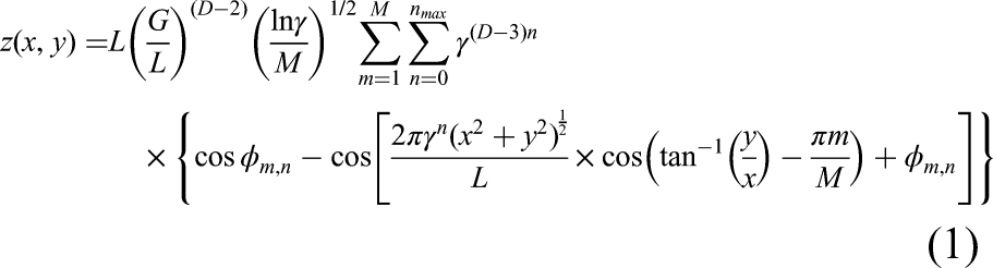
The fractal roughness G is the height scaling parameter, which is independent of frequency within the scale range. Physically, the value of fractal roughness G reflects the surface flatness and higher G values represent the rougher surface topography. The fractal dimension D represents the contribution of the high-frequency and low-frequency components in the surface function
According to Nayak,
41
any surface represents a real random process with spatial frequency variation. The power spectrum density (PSD) method,37,42 which decomposes a rough surface into contributions from different spatial frequencies (wavelength), is an effective method to identify fractal parameters. After determining the fractal parameters, MATLAB is used to generate the surface height
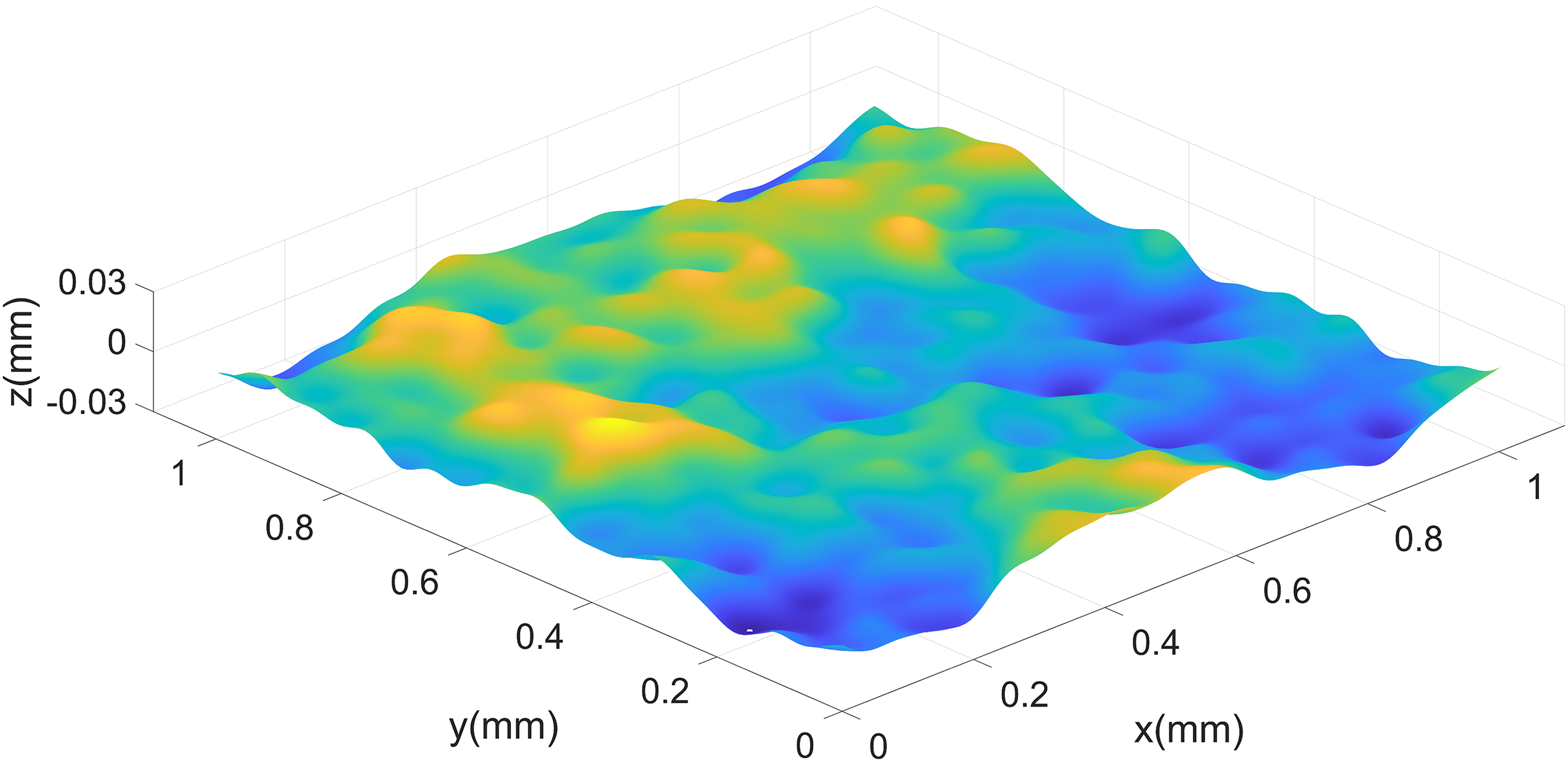
Fractal surface generated by Weierstrass–Mandelbrot (WM) function.
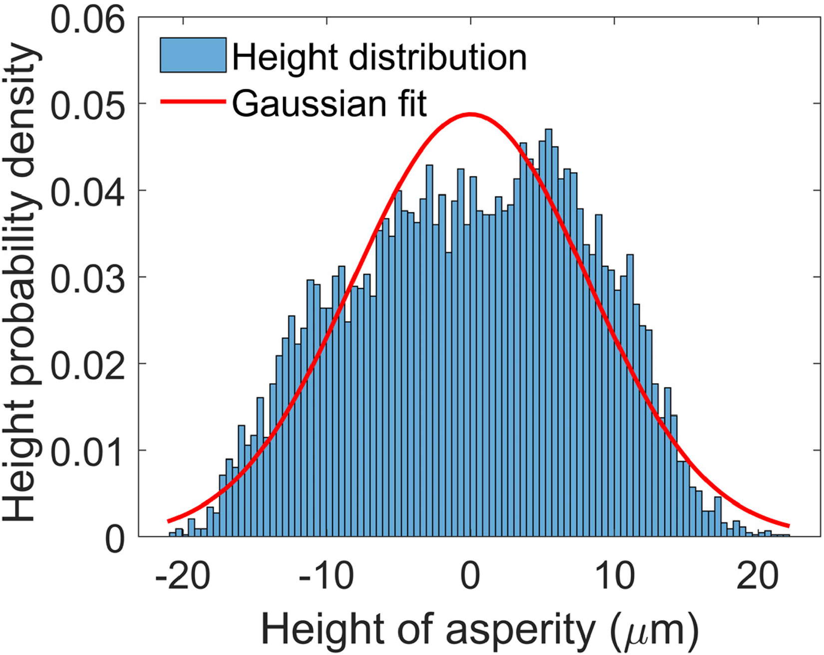
Height probability density (HPD) of the generated fractal surface.
FE modelling
As shown in Figure 1, a 3D fractal rough surface has been generated by equation (1). Then, the coordinates of the fractal rough surface
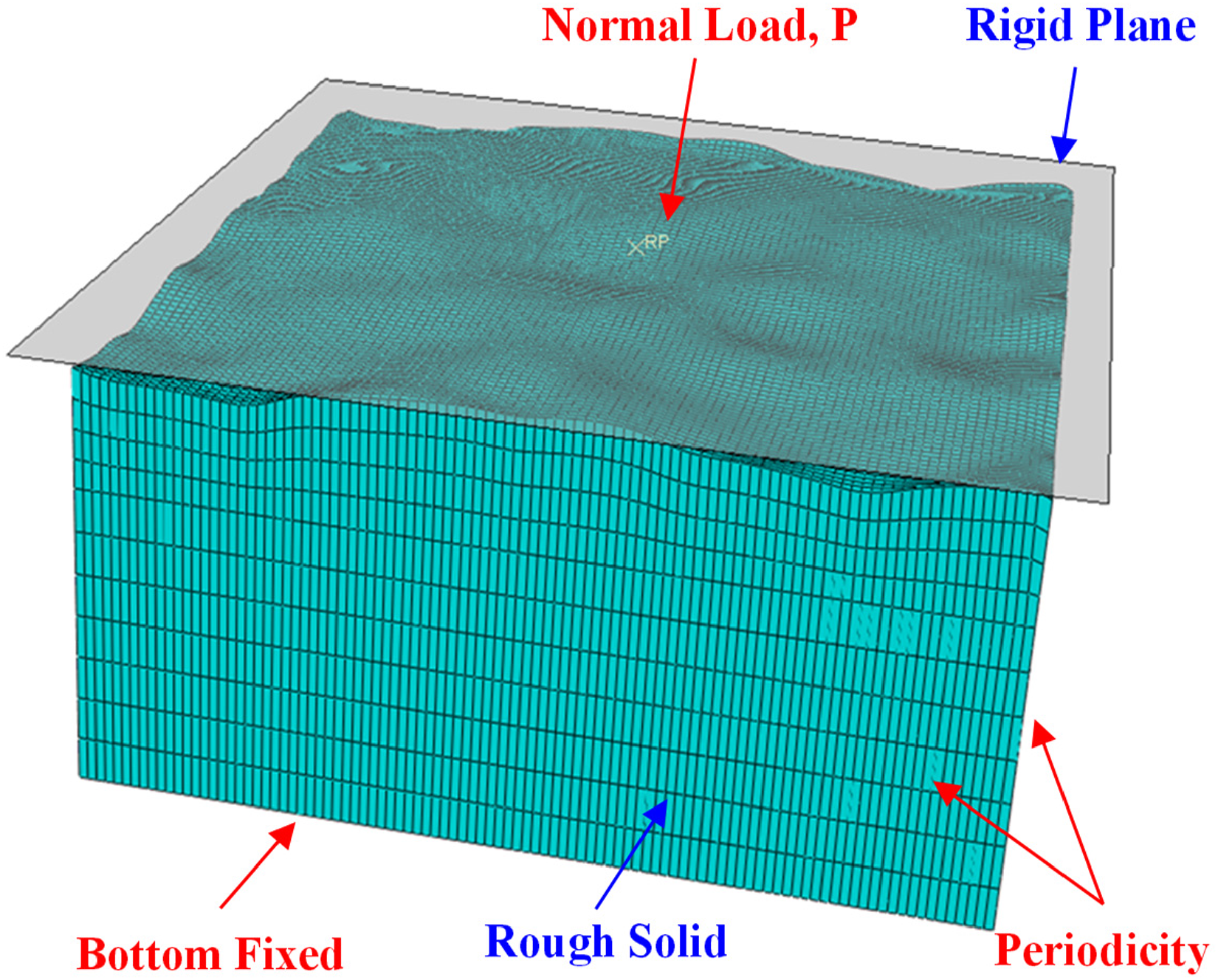
Finite element meshing model for contact between a rigid plane and a rough surface.
The parameters for the rough surface are the same as shown in Figure 1. The mesh resolution of the rough surface is
Simulation cases
According to Zong et al.,
44
three rough surfaces with different roughness levels were machined by the fine grinding process, and the surface topographies were measured by a 3D white light interferometric profilometer. According to the surface topography measurement results by Zong et al.,
44
the surface roughness
Fractal parameters of three rough surfaces.
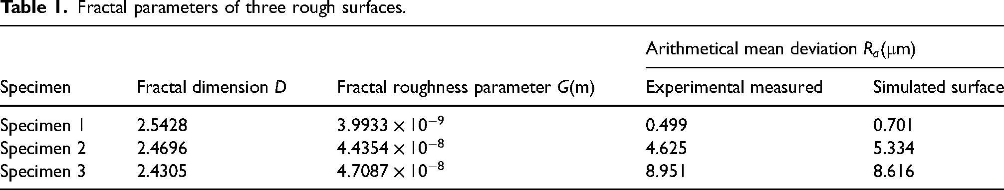
As shown in Figure 4, three fractal rough surfaces were generated using the fractal parameters listed in Table 1. The two-dimensional (2D) rough surface profile at
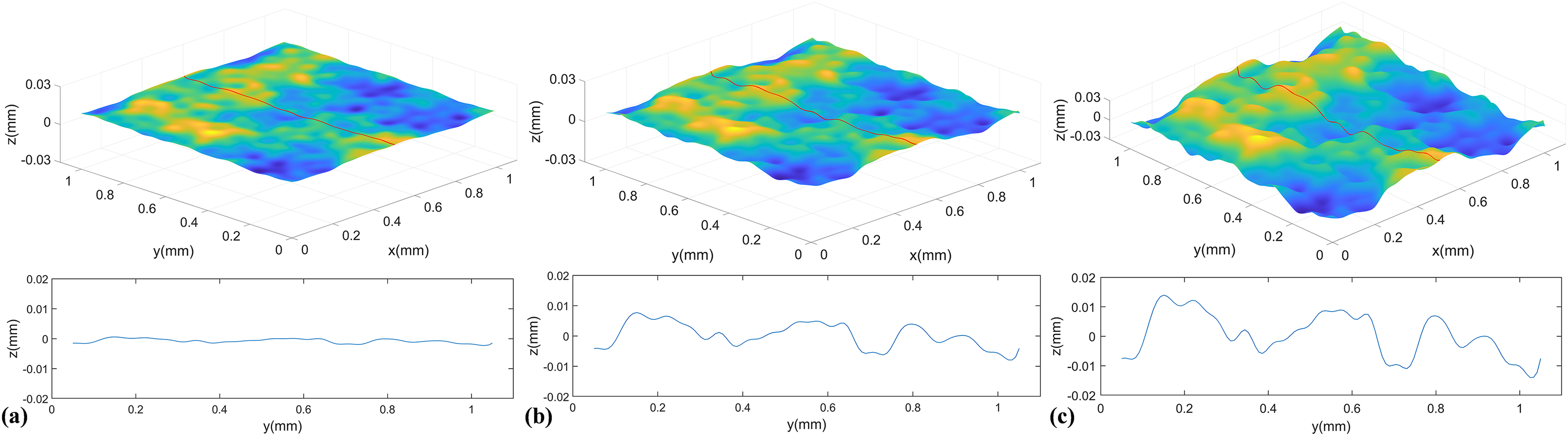
Three fractal rough surfaces with different roughness levels: (a)
Results and discussion
Elastoplastic contact behaviour of rough surfaces
Figure 5 shows the simulated contact pressure of the rough surface with
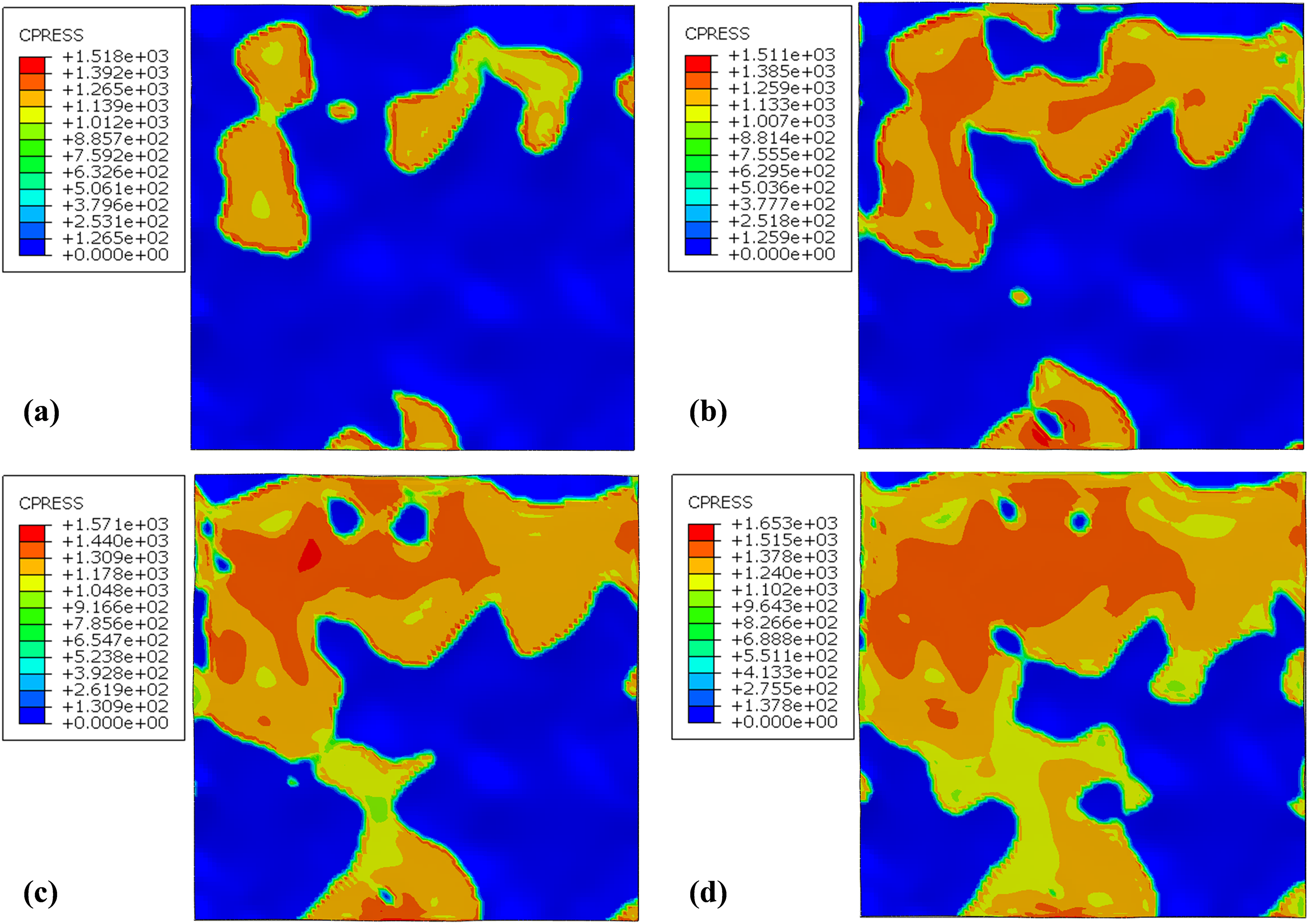
The contact pressure of the rough surface at different normal loads: (a)
The profile height of the rough surface has a significant impact on the contact pressure, which determines the elastoplastic contact status of the surface. The Mises yield criterion 45 is applied to assess whether the surface is elastic or plastic contact. Figure 6 presents the Mises stress at different normal loads, where the blue and red areas are elastically and plastically deformed, respectively. Comparing Figure 6 with Figure 5 it is seen that the projected plastic region is larger than that of the contact region. It is well known that when the asperity is in contact with the rigid plane, a plastically deformed region is first nucleated below the contact region. 46 As the load increases, the plastic region expands to the surface to form an annulus plastic region until the entire contact area is plastically deformed.47,48 When a rough surface is in contact with a rigid plane, the contact between one asperity and the rigid plane first occurs. As load increases, plastic deformation of the asperity continues to develop and the other asperity participates in contact. The neighbouring asperities deform in a similar manner to the former asperity, and the two asperities interact with each other. Consequently, the deformation mechanism of the asperity and the interaction of asperities together result in a larger projected plastic region than the contact area. It is noted that in Figure 6, the Mises stress of some nodes exceeds the yield stress, which is caused by the extrapolation of the integral points to the nodes in the FE model.
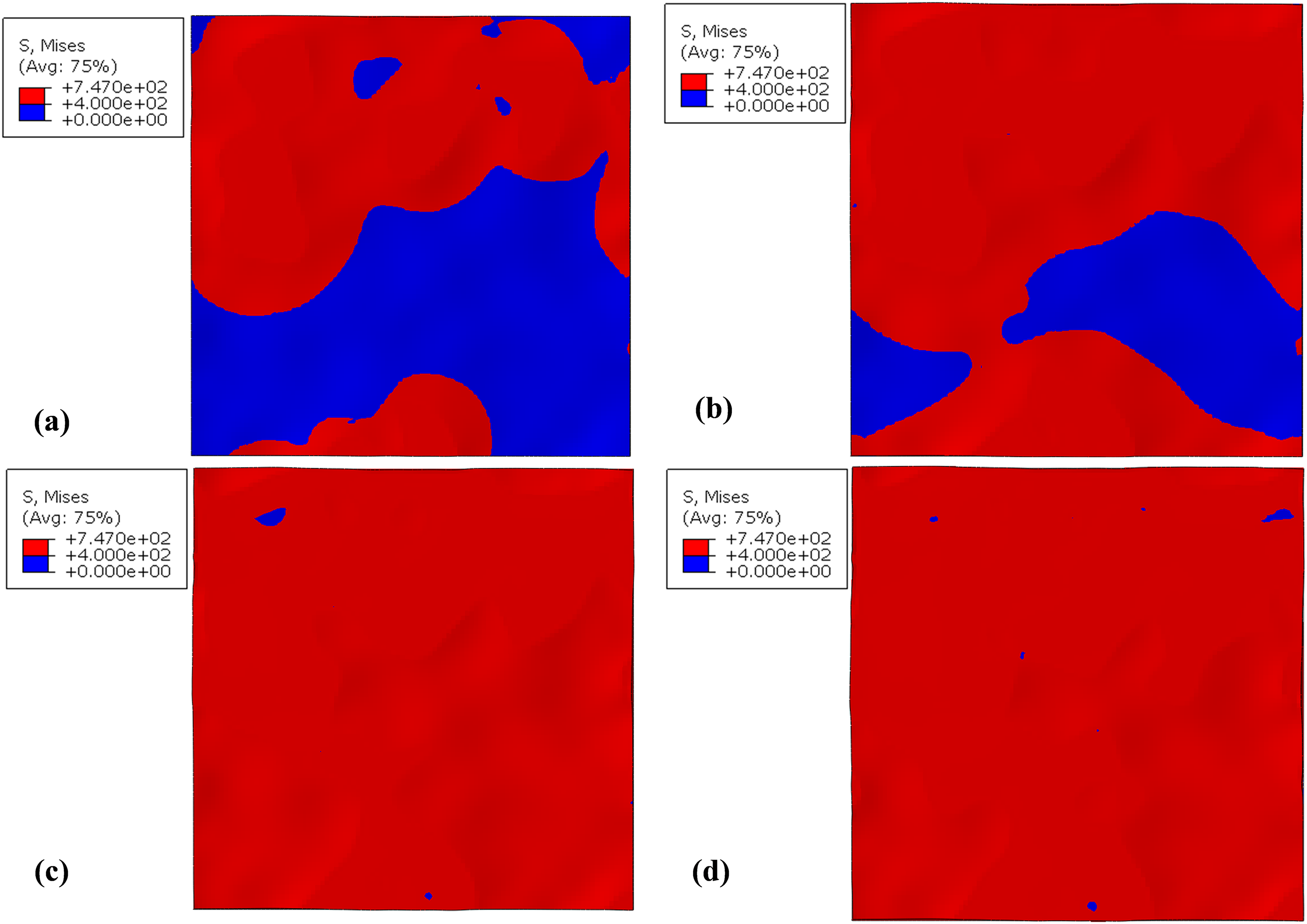
Elastic–plastic contact status of the rough surface at different normal loads: (a)
Based on the simulation results, the dimensionless contact load (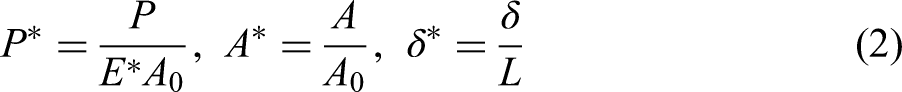
Figure 7 shows the variation of the dimensionless contact area
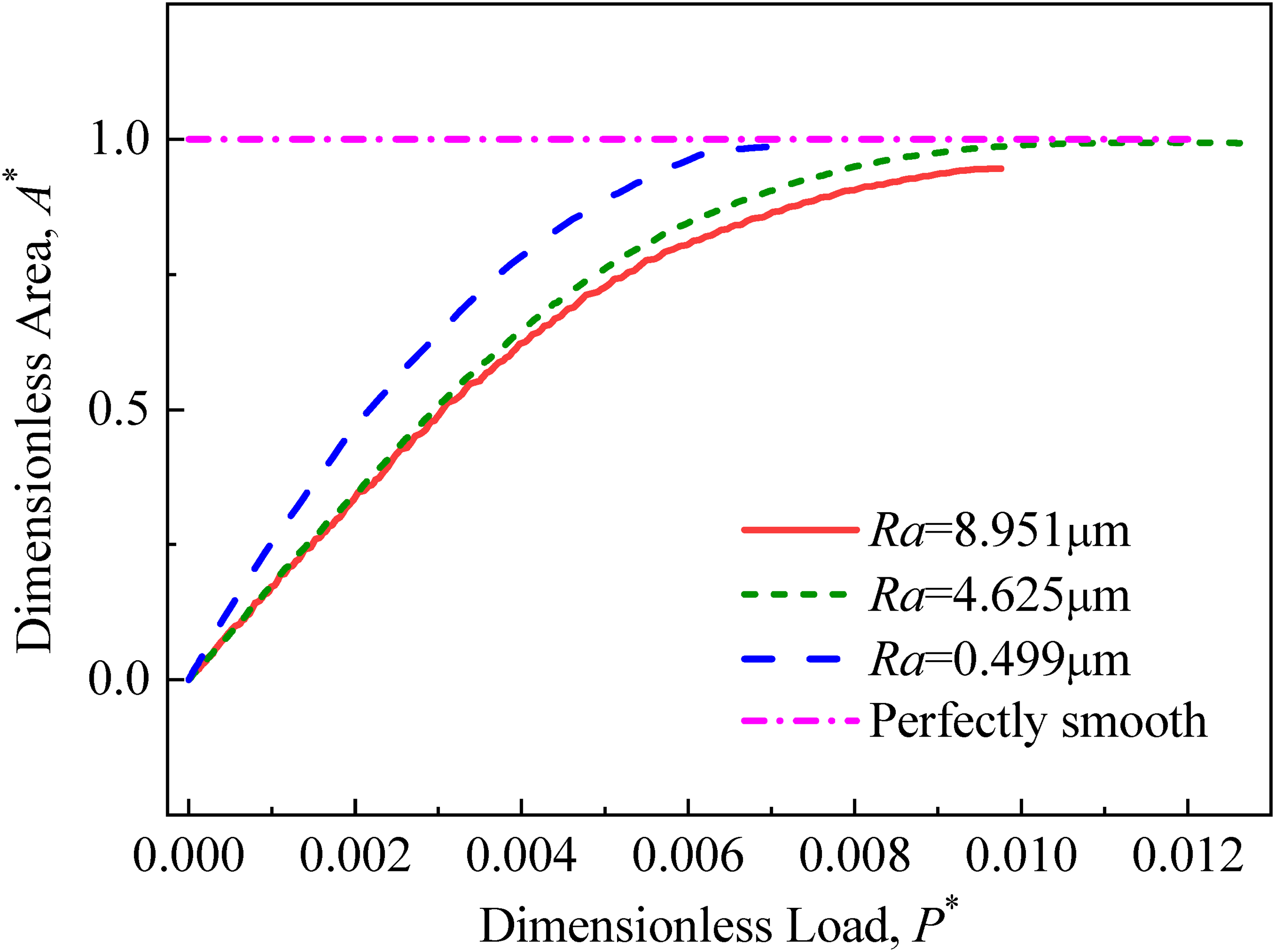
Dimensionless contact area versus dimensionless load for different surfaces.
Figure 8 shows the plots of dimensionless load as a function of dimensionless displacement of the rigid plane and the slope of the load–displacement curve represents the contact stiffness. For a perfectly smooth surface, the contact stiffness exhibits a bilinear behaviour. Before the turning point, only elastic deformation occurs. Following the turning point, the material experiences plastic deformation, resulting in a decrease in stiffness. Due to the contact status involving just linear elastic contact of several asperities, the contact stiffness for rough surfaces grows gradually at the initial loading stage. Some asperities undergo plastic deformation as the load increases, whereas others retain elasticity. During this stage, the contact stiffness is approximately constant with slight fluctuations caused by the randomness of the rough surface. When the load is high enough, the deformable solid body progressively becomes fully plastic, resulting in a further drop in contact stiffness. Finally, the asperity undergoes complete plastic deformation, and thus the contact stiffness of the rough surface approaches that of the smooth surface.
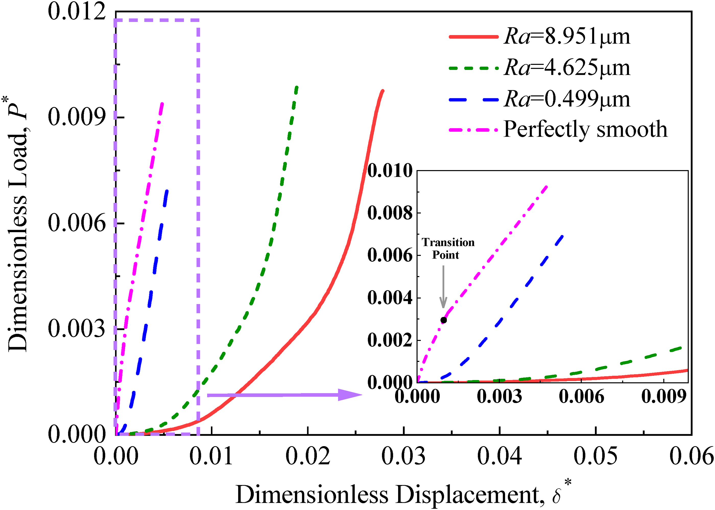
Dimensionless load versus dimensionless displacement for different surfaces.
The variation of the mean contact pressure with dimensionless contact load is shown in Figure 9. The mean contact pressure is the ratio of the normal load to the real contact area. Therefore, the contact pressure of a perfectly smooth surface increases linearly with the load because the contact area is the nominal contact area under any compressive normal load. However, the mean contact pressure of rough surfaces is greater than that of perfectly smooth surfaces because of the stress concentration at the asperity contact spots. For surface with
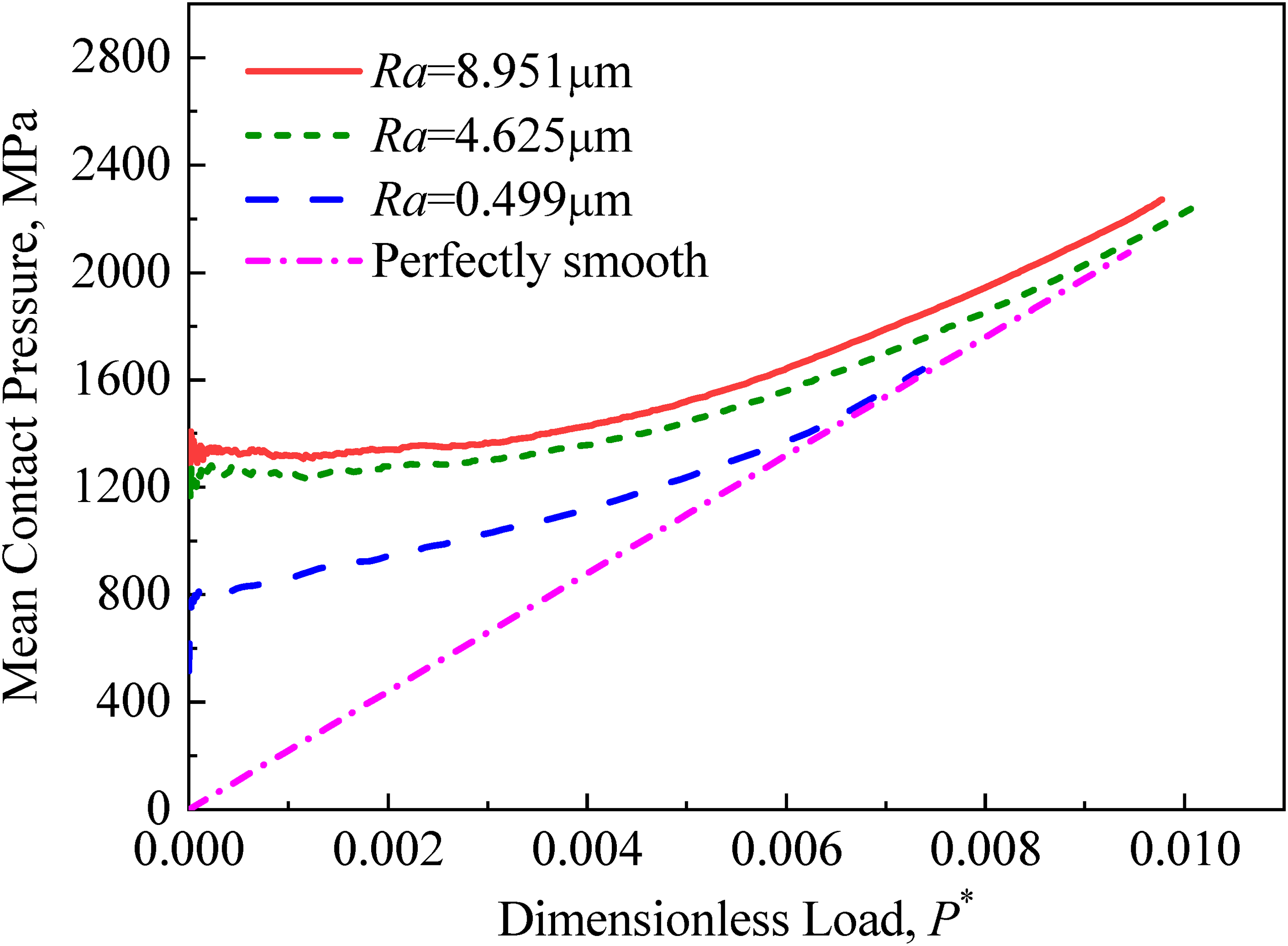
Mean contact pressure versus dimensionless load for different roughness levels.
In the original GW model,
49
plasticity index
Description of contact pressure by statistical method
Statistical modelling of contact pressure
The CPRSS of the field output in software Abaqus describes the contact pressure at each node. The contact pressure data of all contacting nodes are extracted to conduct the statistical analysis. The PDF of contact pressure distribution is determined by the contact pressure data within the contact area, not the entire contact interface. Taking Specimen 2 with
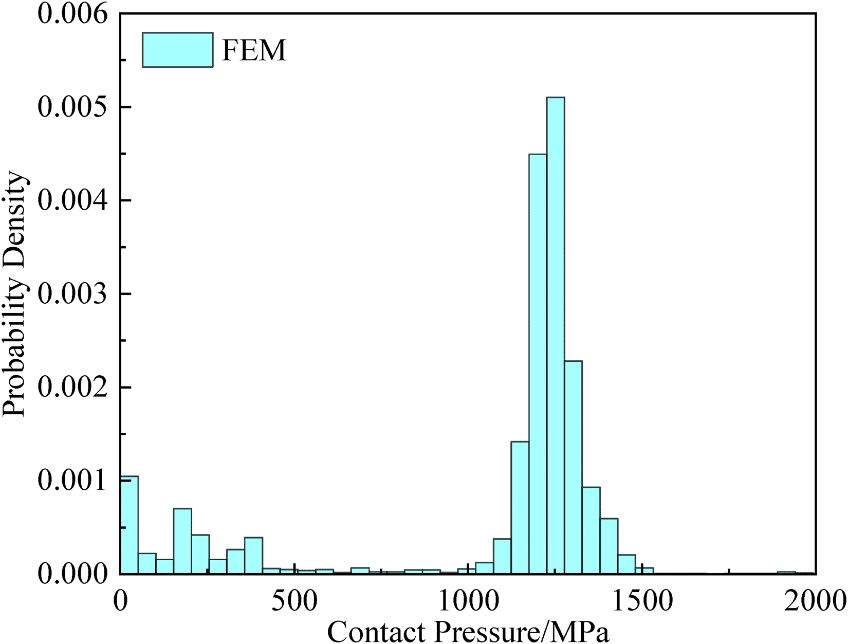
Contact pressure distribution under 400 N preload for Specimen 2.
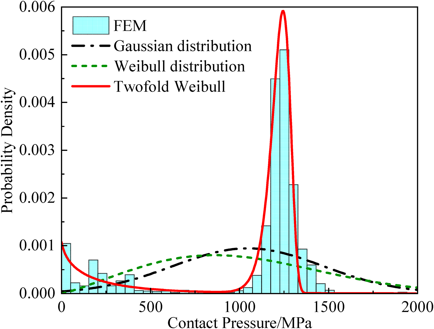
Three popular distributions (Gaussian, Weibull and twofold Weibull mixture) are employed to model the probability distribution function (PDF) and cumulative distribution function (CDF) for the contact pressure data. The Gaussian distribution (normal distribution) and Weibull distribution are extensively used in continuous statistical functions. The formula for the Weibull distribution function with three parameters is written as
The corresponding estimated parameters of Gaussian distribution and Weibull distribution are calculated with the use of the software Matlab by the toolbox function ‘fitdist’. As shown in Figure 11, both Gaussian and Weibull distributions do not fit the contact pressure histogram very well. Noticing the bimodal nature of the histogram, a twofold Weibull mixture model with each representing one type of distribution is proposed to fit the distribution of contact pressure. Mathematically, the bimodal distribution is the superposition of two unimodal distributions. A twofold Weibull mixture model is written as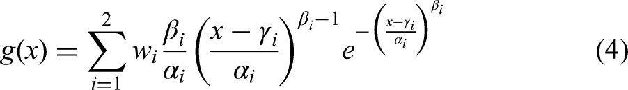
The probability density function of contact pressure.
For simple Weibull distribution, the nonlinear relationship between the sample data x and the corresponding function value 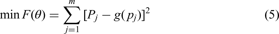
Checking the validity of the twofold Weibull mixture model
The CDFs of the Gaussian distribution and Weibull distribution can be found by Murthy et al.
56
and Ahsanullah et al.
57
and the CDF of the twofold Weibull mixture model (equation (6)) can be derived using its probability density function (equation (4)).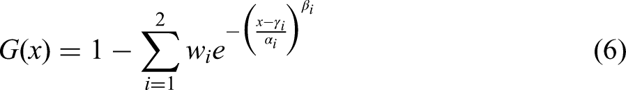
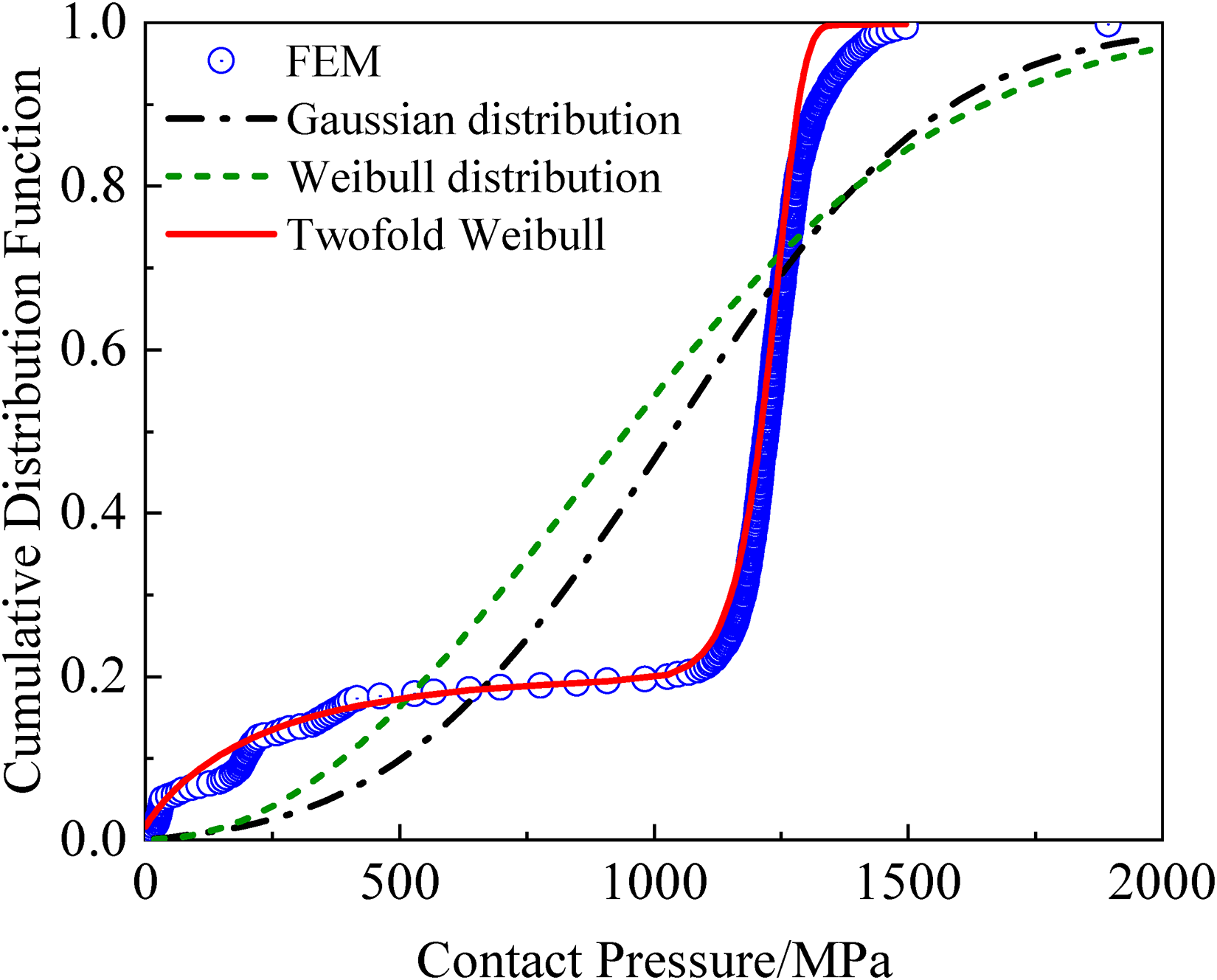
Cumulative distribution function of contact pressure.

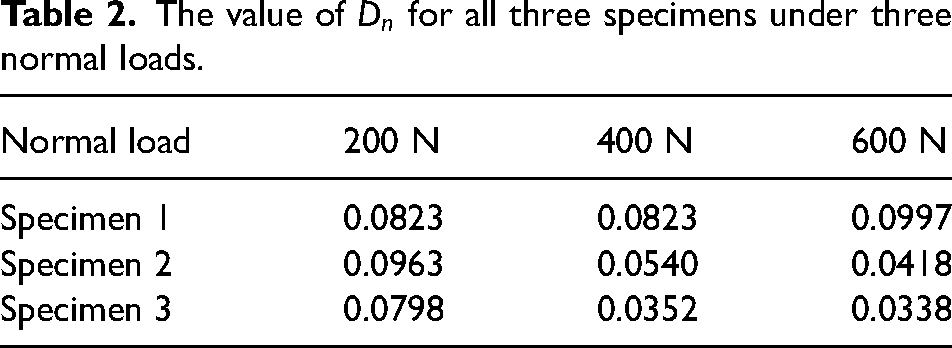
The values of
The value of
Contact pressure distribution characteristics
Effect of load and roughness on contact pressure distribution
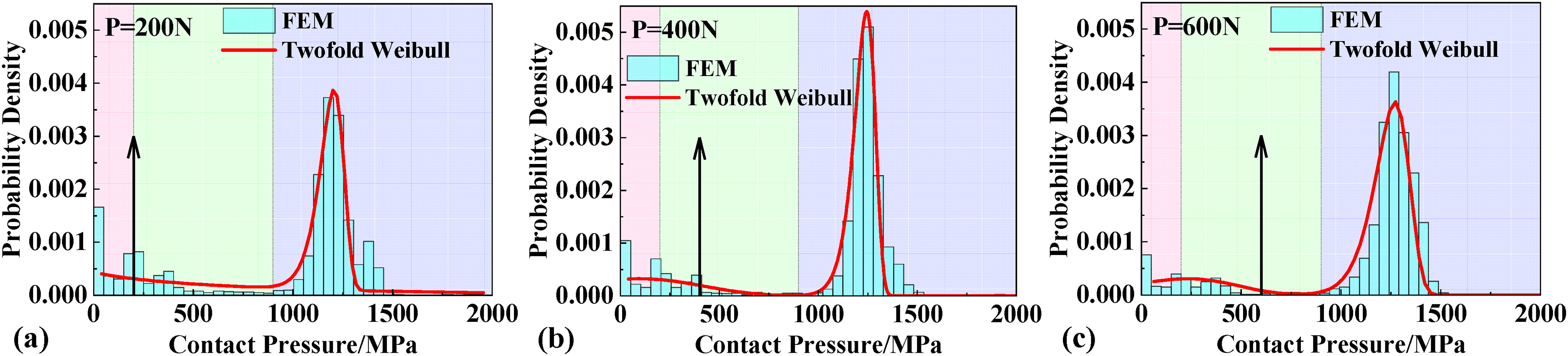
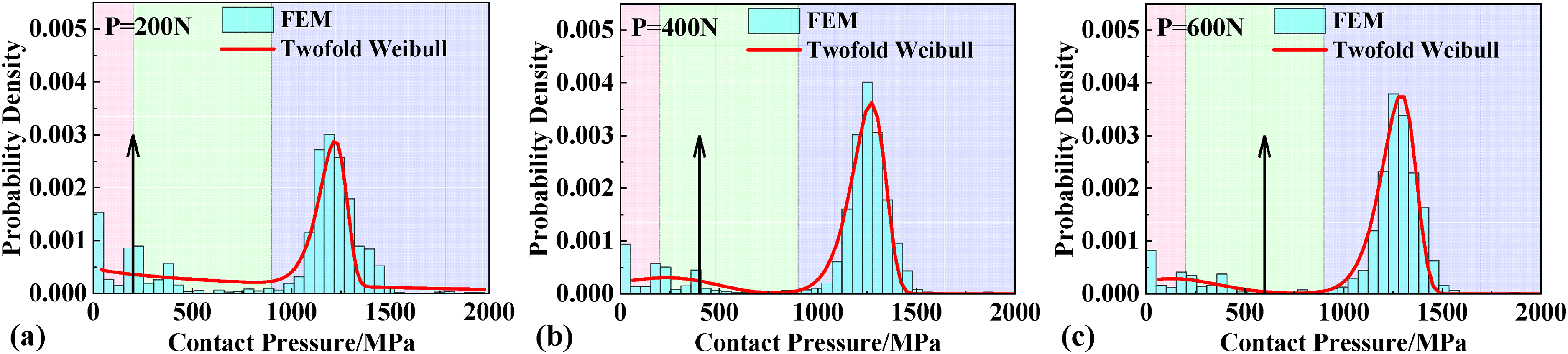
As shown in Figures 13 to 15, the simulated discrete values of contact pressure at varying applied loads for different surfaces are extracted, and statistical analysis is performed to determine the discrete values of probability density. The horizontal axis represents the range of contact pressure. The vertical axis represents the probability density corresponding to the contact pressure. A good agreement is observed between simulated results and the twofold Weibull mixture model for each of the applied normal loads. It is also noted that some fitted curves do not represent well the distribution around 0, which might be related to the optimization process that minimizes the global error without ensuring the minimization of the local error. The contact pressure distribution of a perfectly smooth surface is exactly a uniform distribution. However, as shown in Figures 13 to 15, it is seen that the contact pressure distribution of the rough surface is significantly different from that of the smooth surface. Compared with the Dirac function of the contact pressure PDF for the perfectly smooth surface, the PDF of the contact pressure of the rough surface is broadened with a larger variance towards the low contact pressure. With the increase of roughness, the variability of contact pressure increases and the proportion of high contact pressure increases significantly. The presence of the small contact pressure is mostly attributable to the elastic contact pressure at the margin of the real contact area.
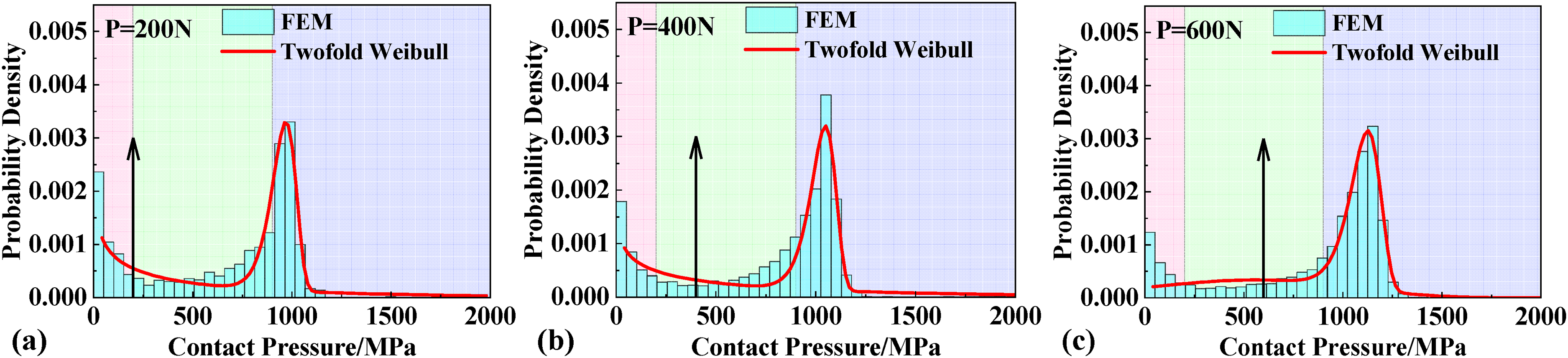
Contact pressure distribution at varying applied loads for
Contact pressure distribution at varying applied loads for
Contact pressure distribution at varying applied loads for
Figure 16 shows the fitting results of twofold Weibull mixture model for different surfaces at varying applied loads. For the same normal contact load, the peak value of the contact pressure probability density moves towards higher contact pressures as the roughness increases. The probability density function changes significantly when the roughness increases from
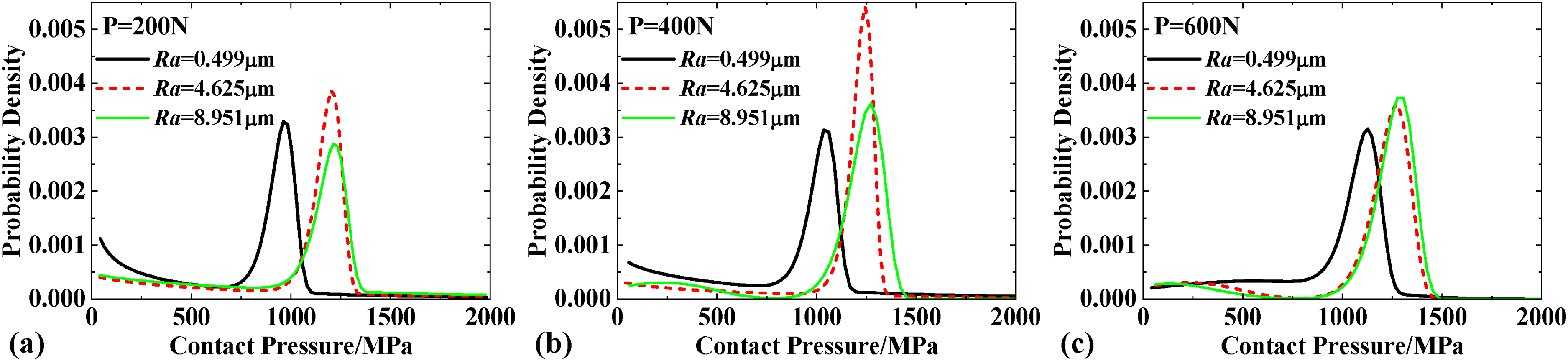
Fitting results of twofold Weibull mixture model for different surfaces: (a)
Effect of yield stress on contact pressure distribution
To analyse the effect of yield stress
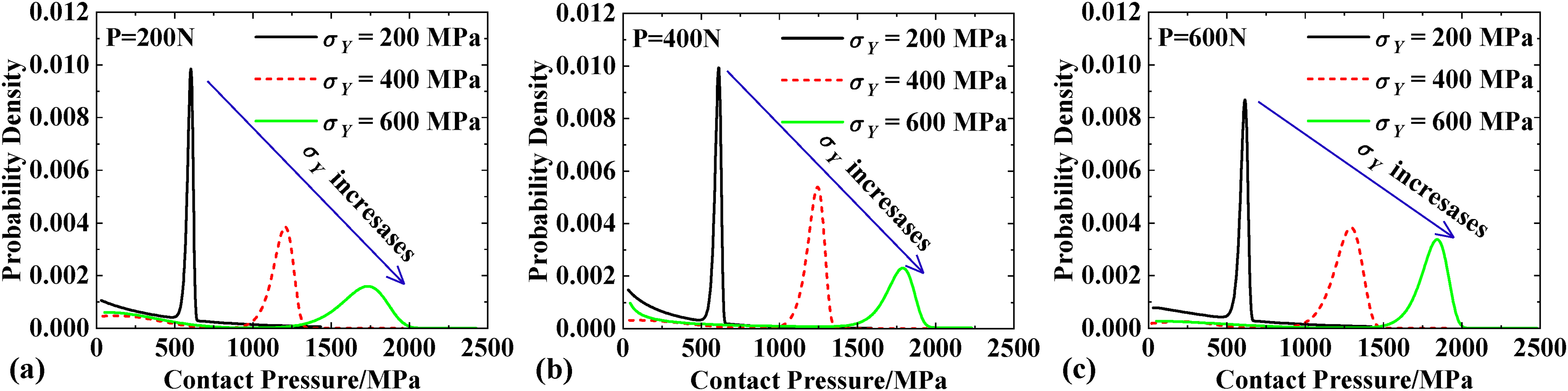
Variation of contact pressure distribution with yield stress: (a)
Conclusions
This work simulated the normal contact behaviour of fractal rough surfaces by employing the FE method. The aim of this article is to obtain a more realistic or physically-based contact pressure distribution form and investigate the effect of roughness and normal load on contact pressure distribution. The fractal rough surface was generated using the modified two-variable WM function. The contact pressure distribution between a fractal rough surface and a rigid plane was investigated by combining the FE method and statistical analysis.
Surface roughness reduces the real contact area, resulting in a completely different relationship between contact pressure and contact load compared to perfectly smooth surfaces, as determined by numerical simulations. Due to the roughness, the contact occurs in a more localized region, which reduces the overall contact stiffness. The mean contact pressure of a perfectly smooth surface increases with the load increasing. In contrast, for rough surfaces, the mean contact pressure initially remains constant as the normal load increases, and when the normal force is sufficiently large, the mean contact pressure converges to the contact case of the perfectly smooth. The probability density distribution of contact pressure is determined using the statistical method and might be approximated as a twofold Weibull distribution.
This article proposed a mathematical description model with a continuous function to explicitly determine the PDF of the contact pressure distribution. In fact, the contact pressure distribution is largely influenced by the geometry of contact bodies as well as the waviness and roughness of surfaces. The influence of geometry deviation and waviness on contact pressure distribution will be considered in the future.
Footnotes
Acknowledgements
The authors would like to acknowledge support from the National Natural Science Foundation of China (Nos. 12072268 and 52105179) and the China Science Challenge project (No. TZ2018007).
Declaration of conflicting interests
The author(s) declared no potential conflicts of interest with respect to the research, authorship, and/or publication of this article.
Funding
The author(s) disclosed receipt of the following financial support for the research, authorship, and/or publication of this article: This work was supported by the National Natural Science Foundation of China (grant no. 12072268 and 52105179).
Appendix A
Figure 18(a) shows the FE model for Specimen 2 (
To analyse the influence of height the height of the bulk, two additional models with height = 0.75 and 1 mm are established for comparative analysis, as shown in Figure 18(c) and (d). Figures 19 and 20 show the comparative results among three FE models with height = 0.5, 0.75 and 1 mm. It is seen that the curve between the contact area and normal load and the contact pressure distribution for the three models are in good agreement. Therefore, it is feasible to investigate the contact pressure distribution using the FE model with height = 0.5 mm.
Since the computation cost is less for surfaces with smaller roughness, three FE models (